Sim: DIFFERENTIABLE SIMULATION FOR SYSTEM IDENTIFICATION AND VISUOMOTOR CONTROL
←
→
Page content transcription
If your browser does not render page correctly, please read the page content below
Published as a conference paper at ICLR 2021

                                        ∇Sim: D IFFERENTIABLE  SIMULATION FOR SYSTEM
                                        IDENTIFICATION AND VISUOMOTOR CONTROL
                                                                           https://gradsim.github.io

                                         Krishna Murthy Jatavallabhula∗ 1,3,4 , Miles Macklin∗2 , Florian Golemo1,3 , Vikram Voleti3,4 , Linda
                                        Petrini3 , Martin Weiss3,4 , Breandan Considine3,5 , Jérôme Parent-Lévesque3,5 , Kevin Xie2,6,7 , Kenny
                                            Erleben8 , Liam Paull1,3,4 , Florian Shkurti6,7 , Derek Nowrouzezahrai3,5 , and Sanja Fidler2,6,7
                                            1
                                                Montreal Robotics and Embodied AI Lab, 2 NVIDIA, 3 Mila, 4 Université de Montréal, 5 McGill,
                                                           6
                                                             University of Toronto, 7 Vector Institute, 8 University of Copenhagen
arXiv:2104.02646v1 [cs.CV] 6 Apr 2021

                                        Figure 1: ∇Sim is a unified differentiable rendering and multiphysics framework that allows solving a range of
                                        control and parameter estimation tasks (rigid bodies, deformable solids, and cloth) directly from images/video.
                                                                                           A BSTRACT
                                                         We consider the problem of estimating an object’s physical properties such as mass,
                                                         friction, and elasticity directly from video sequences. Such a system identification
                                                         problem is fundamentally ill-posed due to the loss of information during image
                                                         formation. Current solutions require precise 3D labels which are labor-intensive
                                                         to gather, and infeasible to create for many systems such as deformable solids
                                                         or cloth. We present ∇Sim, a framework that overcomes the dependence on 3D
                                                         supervision by leveraging differentiable multiphysics simulation and differentiable
                                                         rendering to jointly model the evolution of scene dynamics and image formation.
                                                         This novel combination enables backpropagation from pixels in a video sequence
                                                         through to the underlying physical attributes that generated them. Moreover, our
                                                         unified computation graph – spanning from the dynamics and through the rendering
                                                         process – enables learning in challenging visuomotor control tasks, without relying
                                                         on state-based (3D) supervision, while obtaining performance competitive to or
                                                         better than techniques that rely on precise 3D labels.

                                        1           I NTRODUCTION
                                        Accurately predicting the dynamics and physical characteristics of objects from image sequences is a
                                        long-standing challenge in computer vision. This end-to-end reasoning task requires a fundamental
                                        understanding of both the underlying scene dynamics and the imaging process. Imagine watching a
                                        short video of a basketball bouncing off the ground and ask: “Can we infer the mass and elasticity
                                        of the ball, predict its trajectory, and make informed decisions, e.g., how to pass and shoot?” These
                                        seemingly simple questions are extremely challenging to answer even for modern computer vision
                                        models. The underlying physical attributes of objects and the system dynamics need to be modeled
                                        and estimated, all while accounting for the loss of information during 3D to 2D image formation.
                                        Depending on the assumptions on the scene structre and dynamics, three types of solutions exist:
                                        black, grey, or white box. Black box methods (Watters et al., 2017; Xu et al., 2019b; Janner et al., 2019;
                                        Chang et al., 2016) model the state of a dynamical system (such as the basketball’s trajectory in time)
                                        as a learned embedding of its states or observations. These methods require few prior assumptions
                                        about the system itself, but lack interpretability due to entangled variational factors (Chen et al.,
                                        2016) or due to the ambiguities in unsupervised learning (Greydanus et al., 2019; Cranmer et al.,
                                        2020b). Recently, grey box methods (Mehta et al., 2020) leveraged partial knowledge about the
                                        system dynamics to improve performance. In contrast, white box methods (Degrave et al., 2016;
                                                ∗
                                                    Equal contribution

                                                                                                  1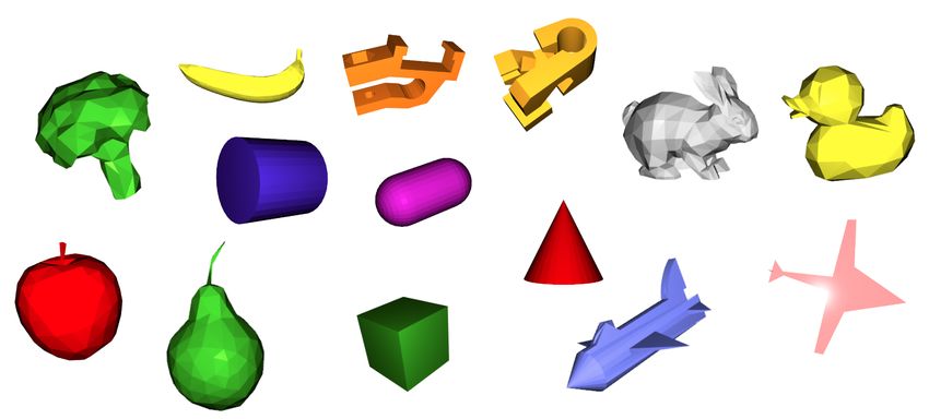
Published as a conference paper at ICLR 2021

Figure 2: ∇Sim: Given video observations of an evolving physical system (e), we randomly initialize scene
object properties (a) and evolve them over time using a differentiable physics engine (b), which generates states.
Our renderer (c) processes states, object vertices and global rendering parameters to produce image frames for
computing our loss. We backprop through this computation graph to estimate physical attributes and controls.
Existing methods rely solely on differentiable physics engines and require supervision in state-space (f), while
∇Sim only needs image-space supervision (g).

Liang et al., 2019; Hu et al., 2020; Qiao et al., 2020) impose prior knowledge by employing explicit
dynamics models, reducing the space of learnable parameters and improving system interpretability.
Most notably in our context, all of these approaches require precise 3D labels – which are labor-
intensive to gather, and infeasible to generate for many systems such as deformable solids or cloth.
We eliminate the dependence of white box dynamics methods on 3D supervision by coupling
explicit (and differentiable) models of scene dynamics with image formation (rendering)1 .
Explicitly modeling the end-to-end dynamics and image formation underlying video observations
is challenging, even with access to the full system state. This problem has been treated in the
vision, graphics, and physics communities (Pharr et al., 2016; Macklin et al., 2014), leading to the
development of robust forward simulation models and algorithms. These simulators are not readily
usable for solving inverse problems, due in part to their non-differentiability. As such, applications of
black-box forward processes often require surrogate gradient estimators such as finite differences
or REINFORCE (Williams, 1992) to enable any learning. Likelihood-free inference for black-box
forward simulators (Ramos et al., 2019; Cranmer et al., 2020a; Kulkarni et al., 2015; Yildirim et al.,
2017; 2015; 2020; Wu et al., 2017b) has led to some improvements here, but remains limited in
terms of data efficiency and scalability to high dimensional parameter spaces. Recent progress in
differentiable simulation further improves the learning dynamics, however we still lack a method for
end-to-end differentiation through the entire simulation process (i.e., from video pixels to physical
attributes), a prerequisite for effective learning from video frames alone.
We present ∇Sim, a versatile end-to-end differentiable simulator that adopts a holistic, unified view
of differentiable dynamics and image formation(cf. Fig. 1,2). Existing differentiable physics engines
only model time-varying dynamics and require supervision in state space (usually 3D tracking). We
additionally model a differentiable image formation process, thus only requiring target information
specified in image space. This enables us to backpropagate (Griewank & Walther, 2003) training
signals from video pixels all the way to the underlying physical and dynamical attributes of a scene.
Our main contributions are:
• ∇Sim, a differentiable simulator that demonstrates the ability to backprop from video pixels to the
  underlying physical attributes (cf. Fig. 2).
• We demonstrate recovering many physical properties exclusively from video observations, including
  friction, elasticity, deformable material parameters, and visuomotor controls (sans 3D supervision)
• A PyTorch framework facilitating interoperability with existing machine learning modules.
We evaluate ∇Sim’s effectiveness on parameter identification tasks for rigid, deformable and thin-
shell bodies, and demonstrate performance that is competitive, or in some cases superior, to current
physics-only differentiable simulators. Additionally, we demonstrate the effectiveness of the gradients
provided by ∇Sim on challenging visuomotor control tasks involving deformable solids and cloth.

2    ∇Sim: A UNIFIED DIFFERENTIABLE SIMULATION ENGINE
Typically, physics estimation and rendering have been treated as disjoint, mutually exclusive tasks.
In this work, we take on a unified view of simulation in general, to compose physics estimation
    1
      Dynamics refers to the laws governing the motion and deformation of objects over time. Rendering refers to
the interaction of these scene elements – including their material properties – with scene lighting to form image
sequences as observed by a virtual camera. Simulation refers to a unified treatment of these two processes.

                                                        2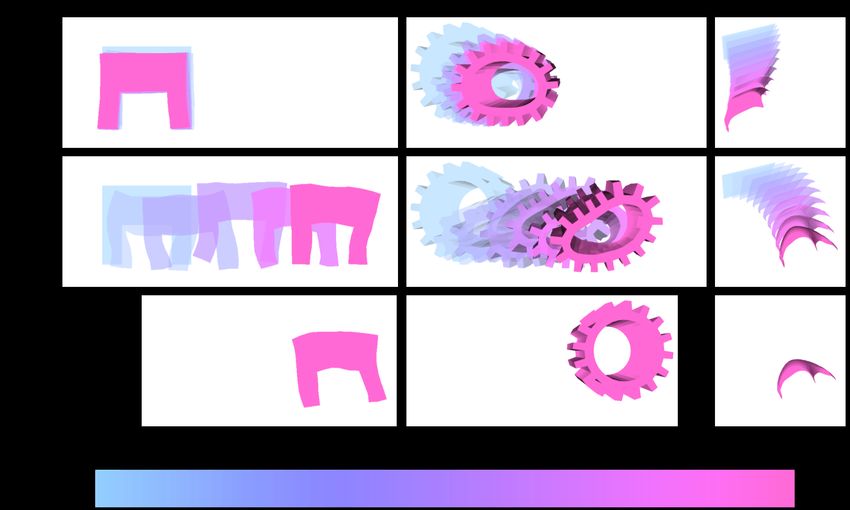
Published as a conference paper at ICLR 2021

and rendering. Formally, simulation is a function Sim : RP × [0, 1] 7→ RH × RW ; Sim(p, t) = I.
Here p ∈ RP is a vector representing the simulation state and parameters (objects, their physical
properties, their geometries, etc.), t denotes the time of simulation (conveniently reparameterized
to be in the interval [0, 1]). Given initial conditions p0 , the simulation function produces an image
I of height H and width W at each timestep t. If this function Sim were differentiable, then the
gradient of Sim(p, t) with respect to the simulation parameters p provides the change in the output
of the simulation from I to I + ∇Sim(p, t)δp due to an infinitesimal perturbation of p by δp .
This construct enables a gradient-based optimizer to estimate physical parameters from video , by
defining a loss function over the image space L(I, .), and descending this loss landscape along a
direction parallel to −∇Sim(.) . To realise this, we turn to the paradigms of computational graphs
and differentiable programming.
∇Sim comprises two main components: a differentiable physics engine that computes the physical
states of the scene at each time instant, and a differentiable renderer that renders the scene to a 2D
image. Contrary to existing differentiable physics (Toussaint et al., 2018; de Avila Belbute-Peres
et al., 2018; Song & Boularias, 2020b;a; Degrave et al., 2016; Wu et al., 2017a; Research, 2020
(accessed May 15, 2020; Hu et al., 2020; Qiao et al., 2020) or differentiable rendering (Loper &
Black, 2014; Kato et al., 2018; Liu et al., 2019; Chen et al., 2019) approaches, we adopt a holistic
view and construct a computational graph spanning them both.

2.1   D IFFERENTIABLE PHYSICS ENGINE

Under Lagrangian mechanics, the state of a physical system can be described in terms of generalized
coordinates q, generalized velocities q̇ = u, and design/model parameters θ. For the purpose of
exposition, we make no distinction between rigid bodies, or deformable solids, or thin-shell models of
cloth, etc. Although the specific choices of coordinates and parameters vary, the simulation procedure
is virtually unchanged. We denote the combined state vector by s(t) = [q(t), u(t)].
The dynamic evolution of the system is governed by second order differential equations (ODEs) of
the form M(s, θ )ṡ = f (s, θ), where M is a mass matrix that depends on the state and parameters.
The forces on the system may be parameterized by design parameters (e.g. Young’s modulus).
Solutions to these ODEs may be obtained through black box numerical integration methods, and
their derivatives calculated through the continuous adjoint method (Chen et al., 2018). However, we
instead consider our physics engine as a differentiable operation that provides an implicit relationship
between a state vector s− = s(t) at the start of a time step, and the updated state at the end of the
time step s+ = s(t + ∆t). An arbitrary discrete time integration scheme can be then be abstracted as
the function g(s− , s+ , θ) = 0 , relating the initial and final system state and the model parameters θ .
Gradients through this dynamical system can be computed by graph-based autodiff frame-
works (Paszke et al., 2019; Abadi et al., 2015; Bradbury et al., 2018), or by program transformation
approaches (Hu et al., 2020; van Merriënboer et al., 2018). Our framework is agnostic to the specifics
of the differentiable physics engine, however in Appendices A through D we detail an efficient
approach based on the source-code transformation of parallel kernels, similar to DiffTaichi (Hu et al.,
2020). In addition, we describe extensions to this framework to support mesh-based tetrahedral
finite-element models (FEMs) for deformable and thin-shell solids. This is important since we require
surface meshes to perform differentiable rasterization as described in the following section.

2.2   D IFFERENTIABLE RENDERING ENGINE

A renderer expects scene description inputs and generates color image outputs, all according to a
sequence of image formation stages defined by the forward graphics pipeline. The scene description
includes a complete geometric descriptor of scene elements, their associated material/reflectance
properties, light source definitions, and virtual camera parameters. The rendering process is not
generally differentiable, as visibility and occlusion events introduce discontinuities. Most interactive
renderers, such as those used in real-time applications, employ a rasterization process to project
3D geometric primitives onto 2D pixel coordinates, resolving these visibility events with non-
differentiable operations.
Our experiments employ two differentiable alternatives to traditional rasterization, SoftRas (Liu
et al., 2019) and DIB-R (Chen et al., 2019), both of which replace discontinuous triangle mesh
edges with smooth sigmoids. This has the effect of blurring triangle edges into semi-transparent

                                                    3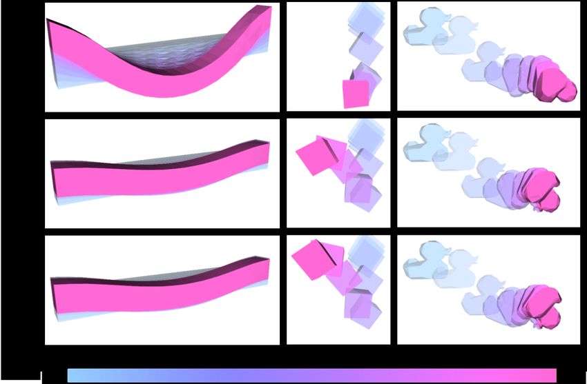
Published as a conference paper at ICLR 2021
boundaries, thereby removing the non-differentiable discontinuity of traditional rasterization. DIB-
R distinguishes between foreground pixels (associated to the principal object being rendered in
the scene) and background pixels (for all other objects, if any). The latter are rendered using the
same technique as SoftRas while the former are rendered by bilinearly sampling a texture using
differentiable UV coordinates.
∇Sim performs differentiable physics simulation and rendering at independent and adjustable rates,
allowing us to trade computation for accuracy by rendering fewer frames than dynamics updates.
3 E XPERIMENTS
We conducted multiple experiments to test the efficacy of ∇Sim on physical parameter identification
from video and visuomotor control, to address the following questions:
• Can we accurately identify physical parameters by backpropagating from video pixels, through the
simulator? (Ans: Yes, very accurately, cf. 3.1)
• What is the performance gap associated with using ∇Sim (2D supervision) vs. differentiable
physics-only engines (3D supervision)? (Ans: ∇Sim is competitive/superior, cf. Tables 1, 2, 3)
• How do loss landscapes differ across differentiable simulators (∇Sim) and their non-differentiable
counterparts? (Ans: Loss landscapes for ∇Sim are smooth, cf. 3.1.3)
• Can we use ∇Sim for visuomotor control tasks? (Ans: Yes, without any 3D supervision, cf. 3.2)
• How sensitive is ∇Sim to modeling assumptions at system level? (Ans: Moderately, cf. Table 4)
Each of our experiments comprises an environment E that applies a particular set of physical forces
and/or constraints, a (differentiable) loss function L that implicitly specifies an objective, and an initial
guess θ0 of the physical state of the simulation. The goal is to recover optimal physics parameters θ∗
that minimize L, by backpropagating through the simulator.
3.1 P HYSICAL PARAMETER ESTIMATION FROM VIDEO
First, we assess the capabilities of ∇Sim to accurately
identify a variety of physical attributes such as mass,
friction, and elasticity from image/video observations.
To the best of our knowledge, ∇Sim is the first study
to jointly infer such fine-grained parameters from
video observations. We also implement a set of com-
petitive baselines that use strictly more information
on the task.
3.1.1 R IGID BODIES ( R I G I D )
Our first environment–rigid–evaluates the accu-
racy of estimating of physical and material attributes
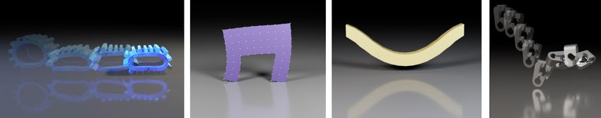
of rigid objects from videos. We curate a dataset Figure 3: Parameter Estimation: For
of 10000 simulated videos generated from varia- deformable experiments, we optimize
tions of 14 objects, comprising primitive shapes such the material properties of a beam to match a video
of a beam hanging under gravity. In the rigid
as boxes, cones, cylinders, as well as non-convex experiments, we estimate contact parameters
shapes from ShapeNet (Chang et al., 2015) and (elasticity/friction) and object density to match a
DexNet (Mahler et al., 2017). With uniformly sam- video (GT). We visualize entire time sequences (t)
pled initial dimensions, poses, velocities, and physi- with color-coded blends.
cal properties (density, elasticity, and friction parame-
ters), we apply a known impulse to the object and record a video of the resultant trajectory. Inference
with ∇Sim is done by guessing an initial mass (uniformly random in the range [2, 12]kg/m3 ), un-
rolling a differentiable simulation using this guess, comparing the rendered out video with the true
video (pixelwise mean-squared error - MSE), and performing gradient descent updates. We refer the
interested reader to the appendix (Sec. G) for more details.
Table 1 shows the results for predicting the mass of an object from video, with a known impulse
applied to it. We use EfficientNet (B0) (Tan & Le, 2019) and resize input frames to 64 × 64. Feature
maps at a resoluition of 4 × 4 × 32 are concatenated for all frames and fed to an MLP with 4 linear
4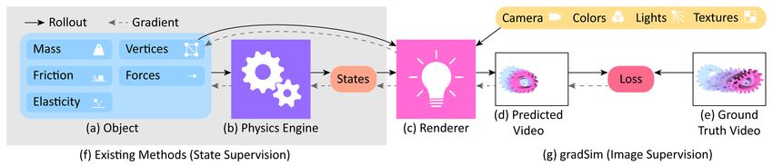
Published as a conference paper at ICLR 2021

  Approach                                    Mean abs.   Abs. Rel.                                 mass     elasticity       friction
                                              err. (kg)     err.       Approach                      m      kd        ke    kf        µ
  Average                                     0.2022      0.1031       Average                     1.7713 3.7145 2.3410 4.1157 0.4463
  Random                                      0.2653      0.1344
  ConvLSTM Xu et al. (2019b)                  0.1347      0.0094       Random                     10.0007 4.18 2.5454 5.0241 0.5558
  PyBullet + REINFORCE Ehsani et al. (2020)   0.0928      0.3668       ConvLSTM Xu et al. (2019b) 0.029    0.14     0.14   0.17     0.096
  DiffPhysics (3D sup.)                       1.35e-9     5.17e-9      DiffPhysics (3D sup.)      1.70e-8 0.036 0.0020 0.0007 0.0107
  ∇Sim                                        2.36e-5     9.01e-5      ∇Sim                       2.87e-4   0.4    0.0026 0.0017 0.0073

Table 1: Mass estimation: ∇Sim obtains precise                        Table 2: Rigid-body parameter estimation: ∇Sim esti-
mass estimates, comparing favourably even with ap-                    mates contact parameters (elasticity, friction) to a high
proaches that require 3D supervision (diffphysics).                   degree of accuracy, despite estimating them from video.
We report the mean abolute error and absolute rela-                   Diffphys. requires accurate 3D ground-truth at 30 FPS. We
tive errors for all approaches evaluated.                             report absolute relative errors for each approach evaluated.

                                                          Deformable solid FEM                       Thin-shell (cloth)
                                               Per-particle mass    Material properties             Per-particle velocity
                                                      m               µ            λ                          v
                Approach                          Rel. MAE       Rel. MAE Rel. MAE                      Rel. MAE
                DiffPhysics (3D Sup.)               0.032          0.0025       0.0024                     0.127
                ∇Sim                                0.048          0.0054       0.0056                     0.026

Table 3: Parameter estimation of deformable objects: We estimate per-particle masses and material properties
(for solid def. objects) and per-particle velocities for cloth. In the case of cloth, there is a perceivable performance
drop in diffphysics, as the center of mass of a cloth is often outside the body, which results in ambiguity.

layers, and trained with an MSE loss. We compare ∇Sim with three other baselines: PyBullet +
REINFORCE (Ehsani et al., 2020; Wu et al., 2015), diff. physics only (requiring 3D supervision), and
a ConvLSTM baseline adopted from Xu et al. (2019b) but with a stronger backbone. The DiffPhysics
baseline is a strict subset of ∇Sim, it only inolves the differentiable physics engine. However, it
needs precise 3D states as supervision, which is the primary factor for its superior performance.
Nevertheless, ∇Sim is able to very precisely estimate mass from video, to a absolute relative error of
9.01e-5, nearly two orders of magnitude better than the ConvLSTM baseline. Two other baselines
are also used: the “Average” baseline always predicts the dataset mean and the “Random” baseline
predicts a random parameter value from the test distribution. All baselines and training details can be
found in Sec. H of the appendix.
To investigate whether analytical differentiability is required, our PyBullet + REINFORCE baseline ap-
plies black-box gradient estimation (Williams, 1992) through a non-differentiable simulator (Coumans
& Bai, 2016–2019), similar to Ehsani et al. (2020). We find this baseline particularly sensitive to
several simulation parameters, and thus worse-performing. In Table 2, we jointly estimate friction
and elasticity parameters of our compliant contact model from video observations alone. The trend
is similar to Table 1, and ∇Sim is able to precisely recover the parameters of the simulation. A few
examples can be seen in Fig. 3.

3.1.2 D EFORMABLE B ODIES ( D E F O R M A B L E )
We conduct a series of experiments to investigate the ability of ∇Sim to recover physical parameters
of deformable solids and thin-shell solids (cloth). Our physical model is parameterized by the per-
particle mass, and Lamé elasticity parameters, as described in in Appendix C.1. Fig. 3 illustrates the
recovery of the elasticity parameters of a beam hanging under gravity by matching the deformation
given by an input video sequence. We found our method is able to accurately recover the parameters
of 100 instances of deformable objects (cloth, balls, beams) as reported in Table 3 and Fig. 3.

3.1.3 S MOOTHNESS OF THE LOSS LANDSCAPE IN ∇Sim
Since ∇Sim is a complex combination of differentiable non-linear components, we analyze the loss
landscape to verify the validity of gradients through the system. Fig. 4 illustrates the loss landscape
when optimizing for the mass of a rigid body when all other physical properties are known.
We examine the image-space mean-squared error (MSE) of a unit-mass cube (1 kg) for a range of
initializations (0.1 kg to 5 kg). Notably, the loss landscape of ∇Sim is well-behaved and conducive
to momentum-based optimizers. Applying MSE to the first and last frames of the predicted and
true videos provides the best gradients. However, for a naive gradient estimator applied to a non-
differentiable simulator (PyBullet + REINFORCE), multiple local minima exist resulting in a very
narrow region of convergence. This explains ∇Sim’s superior performance in Tables 1, 2, 3.

                                                                       5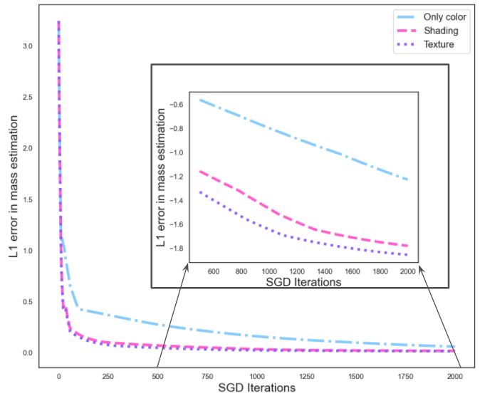
Published as a conference paper at ICLR 2021

           (a) Loss landscape (rigid)                                 (b) Loss landscape (deformable)
Figure 4: Loss landscapes when optimizing for physical attributes using ∇Sim. (Left) When estimating the
mass of a rigid-body with known shape using ∇Sim, despite images being formed by a highly nonlinear
process (simulation), the loss landscape is remarkably smooth, for a range of initialization errors. (Right) when
optimizing for the elasicity parameters of a deformable FEM solid. Both the Lamé parameters λ and µ are set to
1000, where the MSE loss has a unique, dominant minimum. Note that, for fair comparison, the ground-truth for
our PyBullet+REINFORCE baseline was generated using the PyBullet engine.

3.2     V ISUOMOTOR CONTROL
To investigate whether the gradients computed by
∇Sim are meaningful for vision-based tasks, we con-
duct a range of visuomotor control experiments in-
volving the actuation of deformable objects towards
a visual target pose (a single image). In all cases,
we evaluate against diffphysics, which uses a goal
specification and a reward, both defined over the 3D
state-space.

3.2.1    D EFORMABLE SOLIDS
The first example (control-walker) involves a Figure 5: Visuomotor Control: ∇Sim provides
2D walker model. Our goal is to train a neural net- gradients suitable for diverse, complex visuo-
work (NN) control policy to actuate the walker to motor control tasks. For control-fem and
reach a target pose on the right-hand side of an image. control-walker experiments, we train a neu-
                                                        ral network to actuate a soft body towards a target
Our NN consists of one fully connected layer and image (GT). For control-cloth, we optimize
a tanh activation. The network input is a set of 8 the cloth’s initial velocity to hit a target (GT) (spec-
time-varying sinusoidal signals, and the output is a ified as an image), under nonlinear lift/drag forces.
scalar activation value per-tetrahedron. ∇Sim is able
to solve this environment within three iterations of
gradient descent, by minimizing a pixelwise MSE between the last frame of the rendered video and
the goal image as shown in Fig. 5 (lower left).
In our second test, we formulate a more challenging 3D control problem (control-fem) where
the goal is to actuate a soft-body FEM object (a gear) consisting of 1152 tetrahedral elements to
move to a target position as shown in Fig. 5 (center). We use the same NN architecture as in the 2D
walker example, and use the Adam (Kingma & Ba, 2015) optimizer to minimize a pixelwise MSE
loss. We also train a privileged baseline (diffphysics) that uses strong supervision and minimizes the
MSE between the target position and the precise 3D location of the center-of-mass (COM) of the
FEM model at each time step (i.e. a dense reward). We test both diffphysics and ∇Sim against a naive
baseline that generates random activations and plot convergence behaviors in Fig. 6a.
While diffphysics appears to be a strong performer on this task, it is important to note that it uses
explicit 3D supervision at each timestep (i.e. 30 FPS). In contrast, ∇Sim uses a single image as an
implicit target, and yet manages to achieve the goal state, albeit taking a longer number of iterations.

3.2.2    C LOTH ( C O N T R O L - C L O T H )
We design an experiment to control a piece of cloth by optimizing the initial velocity such that it
reaches a pre-specified target. In each episode, a random cloth is spawned, comprising between 64
and 2048 triangles, and a new start/goal combination is chosen.

                                                       6
Published as a conference paper at ICLR 2021
In this challenging setup, we notice that state-based MPC (diffphysics) is often unable to accurately
reach the target. We believe this is due to the underdetermined nature of the problem, since, for
objects such as cloth, the COM by itself does not uniquely determine the configuration of the object.
Visuomotor control on the other hand, provides a more well-defined problem. An illustration of the
task is presented in Fig. 5 (column 3), and the convergence of the methods shown in Fig. 6b.
(a) Results of various approaches on the control-fem (b) Results on control-cloth environment (5
environment (6 randomseeds; each randomseed corre- randomseeds; each controls the dimensions and ini-
sponds to a different goal configuration). While diff- tial/target poses of the cloth). diffphysics converges
physics performs well, it assumes strong 3D supervision. to a suboptimal solution due to ambiguity in specify-
In contrast, ∇Sim is able to solve the task by using just a ing the pose of a cloth via its center-of-mass. ∇Sim
single image of the target configuration. solves the environment using a single target image.
Figure 6: Convergence Analysis: Performance of ∇Sim on visuomotor control using image-based supervision,
3D supervision, and random policies.
3.3 I MPACT OF IMPERFECT DYNAMICS AND RENDERING MODELS
Being a white box method, the performance of ∇Sim relies on the choice of dynamics and rendering
models employed. An immediate question that arises is “how would the performance of ∇Sim
be impacted (if at all) by such modeling choices.” We conduct multiple experiments targeted at
investigating modelling errors and summarize them in Table 4 (left).
We choose a dataset comprising 90 objects equally representing rigid, deformable, and cloth types.
By not modeling specific dynamics and rendering phenomena, we create the following 5 variants of
our simulator.
1. Unmodeled friction: We model all collisions as being frictionless.
2. Unmodeled elasticity: We model all collisions as perfectly elastic.
3. Rigid-as-deformable: All rigid objects in the dataset are modeled as deformable objects.
4. Deformable-as-rigid: All deformable objects in the dataset are modeled as rigid objects.
5. Photorealistic render: We employ a photorealistic renderer—as opposed to ∇Sim’s differentiable
rasterizers—in generating the target images.
In all cases, we evaluate the accuracy with which the mass of the target object is estimated from
a target video sequence devoid of modeling discrepancies. In general, we observe that imperfect
dynamics models (i.e. unmodeled friction and elasticity, or modeling a rigid object as deformable or
vice-versa) have a more profound impact on parameter identification compared to imperfect renderers.
3.3.1 U NMODELED DYNAMICS PHENOMENON
From Table 4 (left), we observe a noticeable performance drop when dynamics effects go unmodeled.
Expectedly, the repurcussions of incorrect object type modeling (Rigid-as-deformable, Deformable-
as-rigid) are more severe compared to unmodeled contact parameters (friction, elasticity). Modeling
a deformable body as a rigid body results in irrecoverable deformation parameters and has the most
severe impact on the recovered parameter set.
3.3.2 U NMODELED RENDERING PHENOMENON
We also independently investigate the impact of unmodeled rendering effects (assuming perfect
dynamics). We indepenently render ground-truth images and object foreground masks from a
photorealistic renderer (Pharr et al., 2016). We use these photorealistic renderings for ground-truth
7Published as a conference paper at ICLR 2021
and perform physical parameter estimation from video. We notice that the performance obtained
under this setting is superior compared to ones with dynamics model imperfections.
Mean Rel. Abs. Err. Tetrahedra (#) Forward (DP) Forward (DR) Backward (DP) Backward (DP + DR)
Unmodeled friction 0.1866 100 9057 Hz 3504 Hz 3721 Hz 3057 Hz
Unmodeled elasticity 0.2281 200 9057 Hz 3478 Hz 3780 Hz 2963 Hz
400 8751 Hz 3357 Hz 3750 Hz 1360 Hz
Rigid-as-deformable 0.3462
1000 4174 Hz 1690 Hz 1644 Hz 1041 Hz
Deformable-as-rigid 0.4974 2000 3967 Hz 1584 Hz 1655 Hz 698 Hz
Photorealistic render 0.1793 5000 3871 Hz 1529 Hz 1553 Hz 424 Hz
Perfect model 0.1071 10000 3721 Hz 1500 Hz 1429 Hz 248 Hz
Table 4: (Left) Impact of imperfect models: The accuracy of physical parameters estimated by ∇Sim is
impacted by the choice of dynamics and graphics (rendering) models. We find that the system is more sensitive
to the choice of dynamics models than to the rendering engine used. (Right) Timing analysis: We report runtime
in simulation steps / second (Hz). ∇Sim is significantly faster than real-time, even for complex geometries.
3.3.3 I MPACT OF SHADING AND TEXTURE CUES
Although our work does not attempt to bridge the
reality gap, we show early prototypes to assess phe-
nomena such as shading/texture. Fig. 7 shows the
accuracy over time for mass estimation from video.
We evaluate three variants of the renderer - “Only
color”, “Shading”, and “Texture”. The “Only color”
variant renders each mesh element in the same color
regardless of the position and orientation of the light
source. The “Shading” variant implements a Phong
shading model and can model specular and diffuse
reflections. The “Texture” variant also applies a non-
uniform texture sampled from ShapeNet (Chang et al.,
2015). We notice that shading and texture cues signif-
icantly improve convergence speed. This is expected, Figure 7: Including shading and texture cues
as vertex colors often have very little appearance cues lead to faster convergence. Inset plot has a log-
inside the object boundaries, leading to poor corre- arithmic Y-axis.
spondences between the rendered and ground-truth
images. Furthermore, textures seem to offer slight improvements in convergence speed over shaded
models, as highlighted by the inset (log scale) plot in Fig. 7.
3.3.4 T IMING ANALYSIS
Table 4 (right) shows simulation rates for the forward and backward passes of each module. We
report forward and backward pass rates separately for the differentiable physics (DP) and the
differentiable rendering (DR) modules. The time complexity of ∇Sim is a function of the number of
tetrahedrons and/or triangles. We illustrate the arguably more complex case of deformable object
simulation for varying numbers of tetrahedra (ranging from 100 to 10000). Even in the case of 10000
tetrahedra—enough to contruct complex mesh models of multiple moving objects—∇Sim enables
faster-than-real-time simulation (1500 steps/second).
4 R ELATED WORK
Differentiable physics simulators have seen significant attention and activity, with efforts centered
around embedding physics structure into autodifferentiation frameworks. This has enabled differ-
entiation through contact and friction models (Toussaint et al., 2018; de Avila Belbute-Peres et al.,
2018; Song & Boularias, 2020b;a; Degrave et al., 2016; Wu et al., 2017a; Research, 2020 (accessed
May 15, 2020), latent state models (Guen & Thome, 2020; Schenck & Fox, 2018; Jaques et al., 2020;
Heiden et al., 2019), volumetric soft bodies (Hu et al., 2019; 2018; Liang et al., 2019; Hu et al.,
2020), as well as particle dynamics (Schenck & Fox, 2018; Li et al., 2019; 2020; Hu et al., 2020). In
contrast, ∇Sim addresses a superset of simulation scenarios, by coupling the physics simulator with a
differentiable rendering pipeline. It also supports tetrahedral FEM-based hyperelasticity models to
simulate deformable solids and thin-shells.
Recent work on physics-based deep learning injects structure in the latent space of the dynamics
using Lagrangian and Hamiltonian operators (Greydanus et al., 2019; Chen et al., 2020; Toth et al.,
8Published as a conference paper at ICLR 2021
2020; Sanchez-Gonzalez et al., 2019; Cranmer et al., 2020b; Zhong et al., 2020), by explicitly
conserving physical quantities, or with ground truth supervision (Asenov et al., 2019; Wu et al., 2016;
Xu et al., 2019b).
Sensor readings have been used to predicting the effects of forces applied to an object in models of
learned (Fragkiadaki et al., 2016; Byravan & Fox, 2017) and intuitive physics (Ehsani et al., 2020;
Mottaghi et al., 2015; 2016; Gupta et al., 2010; Ehrhardt et al., 2018; Yu et al., 2015; Battaglia et al.,
2013; Mann et al., 1997; Innamorati et al., 2019; Standley et al., 2017). This also includes approaches
that learn to model multi-object interactions (Watters et al., 2017; Xu et al., 2019b; Janner et al.,
2019; Ehrhardt et al., 2017; Chang et al., 2016; Agrawal et al., 2016). In many cases, intuitive physics
approaches are limited in their prediction horizon and treatment of complex scenes, as they do not
sufficiently accurately model the 3D geometry nor the object properties. System identification based
on parameterized physics models (Salzmann & Urtasun, 2011; Brubaker et al., 2010; Kozlowski,
1998; Wensing et al., 2018; Brubaker et al., 2009; Bhat et al., 2003; 2002; Liu et al., 2005; Grzeszczuk
et al., 1998; Sutanto et al., 2020; Wang et al., 2020; 2018a) and inverse simulation (Murray-Smith,
2000) are closely related areas.
There is a rich literature on neural image synthesis, but we focus on methods that model the 3D
scene structure, including voxels (Henzler et al., 2019; Paschalidou et al., 2019; Smith et al., 2018b;
Nguyen-Phuoc et al., 2018; Gao et al., 2020), meshes (Smith et al., 2020; Wang et al., 2018b; Groueix
et al., 2018; Alhaija et al., 2018; Zhang et al., 2021), and implicit shapes (Xu et al., 2019a; Chen
& Zhang, 2019; Michalkiewicz et al., 2019; Niemeyer et al., 2020; Park et al., 2019; Mescheder
et al., 2019; Takikawa et al., 2021). Generative models condition the rendering process on samples
of the 3D geometry (Liao et al., 2019). Latent factors determining 3D structure have also been
learned in generative models (Chen et al., 2016; Eslami et al., 2018). Additionally, implicit neural
representations that leverage differentiable rendering have been proposed (Mildenhall et al., 2020;
2019) for realistic view synthesis. Many of these representations have become easy to manipulate
through software frameworks like Kaolin (Jatavallabhula et al., 2019), Open3D (Zhou et al., 2018),
and PyTorch3D (Ravi et al., 2020).
Differentiable rendering allows for image gradients to be computed w.r.t. the scene geometry,
camera, and lighting inputs. Variants based on the rasterization paradigm (NMR (Kato et al., 2018),
OpenDR (Loper & Black, 2014), SoftRas (Liu et al., 2019)) blur the edges of scene triangles prior to
image projection to remove discontinuities in the rendering signal. DIB-R (Chen et al., 2019) applies
this idea to background pixels and proposes an interpolation-based rasterizer for foreground pixels.
More sophisticated differentiable renderers can treat physics-based light transport processes (Li et al.,
2018; Nimier-David et al., 2019) by ray tracing, and more readily support higher-order effects such
as shadows, secondary light bounces, and global illumination.
5 C ONCLUSION
We presented ∇Sim, a versatile differentiable simulator that enables system identification from
videos by differentiating through physical processes governing dyanmics and image formation. We
demonstrated the benefits of such a holistic approach by estimating physical attributes for time-
evolving scenes with complex dynamics and deformations, all from raw video observations. We
also demonstrated the applicability of this efficient and accurate estimation scheme on end-to-end
visuomotor control tasks. The latter case highlights ∇Sim’s efficient integration with PyTorch,
facilitating interoperability with existing machine learning modules. Interesting avenues for future
work include extending our differentiable simulation to contact-rich motion, articulated bodies and
higher-fidelity physically-based renderers – doing so takes us closer to operating in the real-world.
ACKNOWLEDGEMENTS
KM and LP thank the IVADO fundamental research project grant for funding. FG thanks CIFAR for
project funding under the Catalyst program. FS and LP acknowledge partial support from NSERC.
9Published as a conference paper at ICLR 2021
R EFERENCES
Martín Abadi, Ashish Agarwal, Paul Barham, Eugene Brevdo, Zhifeng Chen, Craig Citro, Greg S.
Corrado, Andy Davis, Jeffrey Dean, Matthieu Devin, Sanjay Ghemawat, Ian Goodfellow, Andrew
Harp, Geoffrey Irving, Michael Isard, Yangqing Jia, Rafal Jozefowicz, Lukasz Kaiser, Manjunath
Kudlur, Josh Levenberg, Dan Mané, Rajat Monga, Sherry Moore, Derek Murray, Chris Olah, Mike
Schuster, Jonathon Shlens, Benoit Steiner, Ilya Sutskever, Kunal Talwar, Paul Tucker, Vincent
Vanhoucke, Vijay Vasudevan, Fernanda Viégas, Oriol Vinyals, Pete Warden, Martin Wattenberg,
Martin Wicke, Yuan Yu, and Xiaoqiang Zheng. TensorFlow: Large-scale machine learning on
heterogeneous systems, 2015. URL http://tensorflow.org/. Software available from
tensorflow.org. 3, 17
Pulkit Agrawal, Ashvin Nair, Pieter Abbeel, Jitendra Malik, and Sergey Levine. Learning to poke by
poking: Experiential learning of intuitive physics. Neural Information Processing Systems, 2016. 9
Hassan Abu Alhaija, Siva Karthik Mustikovela, Andreas Geiger, and Carsten Rother. Geometric
image synthesis. In Proceedings of Computer Vision and Pattern Recognition, 2018. 9
Martin Asenov, Michael Burke, Daniel Angelov, Todor Davchev, Kartic Subr, and Subramanian
Ramamoorthy. Vid2Param: Modelling of dynamics parameters from video. IEEE Robotics and
Automation Letters, 2019. 9
Peter W. Battaglia, Jessica B. Hamrick, and Joshua B. Tenenbaum. Simulation as an engine of physical
scene understanding. Proceedings of the National Academy of Sciences, 110(45):18327–18332,
2013. ISSN 0027-8424. doi: 10.1073/pnas.1306572110. 9
Kiran S Bhat, Steven M Seitz, Jovan Popović, and Pradeep K Khosla. Computing the physical
parameters of rigid-body motion from video. In Proceedings of the European Conference on
Computer Vision, 2002. 9
Kiran S Bhat, Christopher D Twigg, Jessica K Hodgins, Pradeep Khosla, Zoran Popovic, and Steven M
Seitz. Estimating cloth simulation parameters from video. In ACM SIGGRAPH/Eurographics
Symposium on Computer Animation, 2003. 9
James Bradbury, Roy Frostig, Peter Hawkins, Matthew James Johnson, Chris Leary, Dougal Maclau-
rin, and Skye Wanderman-Milne. JAX: composable transformations of Python+NumPy programs,
2018. URL http://github.com/google/jax. 3, 17
Robert Bridson, Sebastian Marino, and Ronald Fedkiw. Simulation of clothing with folds and
wrinkles. In ACM SIGGRAPH 2005 Courses, 2005. 17
Marcus Brubaker, David Fleet, and Aaron Hertzmann. Physics-based person tracking using the
anthropomorphic walker. International Journal of Computer Vision, 87:140–155, 03 2010. 9
Marcus A Brubaker, Leonid Sigal, and David J Fleet. Estimating contact dynamics. In Proceedings
of International Conference on Computer Vision, 2009. 9
Arunkumar Byravan and Dieter Fox. SE3-Nets: Learning rigid body motion using deep neural
networks. IEEE International Conference on Robotics and Automation (ICRA), 2017. 9
Angel X Chang, Thomas Funkhouser, Leonidas Guibas, Pat Hanrahan, Qixing Huang, Zimo Li,
Silvio Savarese, Manolis Savva, Shuran Song, Hao Su, et al. ShapeNet: An information-rich 3d
model repository. arXiv preprint arXiv:1512.03012, 2015. 4, 8
Michael B. Chang, Tomer Ullman, Antonio Torralba, and Joshua B. Tenenbaum. A compositional
object-based approach to learning physical dynamics. International Conference on Learning
Representations, 2016. 1, 9
Tian Qi Chen, Yulia Rubanova, Jesse Bettencourt, and David K Duvenaud. Neural ordinary differen-
tial equations. In Neural Information Processing Systems, 2018. 3, 17
Wenzheng Chen, Jun Gao, Huan Ling, Edward Smith, Jaakko Lehtinen, Alec Jacobson, and Sanja
Fidler. Learning to predict 3d objects with an interpolation-based differentiable renderer. Neural
Information Processing Systems, 2019. 3, 9, 19
10Published as a conference paper at ICLR 2021
Xi Chen, Yan Duan, Rein Houthooft, John Schulman, Ilya Sutskever, and Pieter Abbeel. InfoGAN:
Interpretable representation learning by information maximizing generative adversarial nets. Neural
Information Processing Systems, 2016. 1, 9
Zhengdao Chen, Jianyu Zhang, Martin Arjovsky, and Léon Bottou. Symplectic recurrent neural
networks. In International Conference on Learning Representations, 2020. 8
Zhiqin Chen and Hao Zhang. Learning implicit fields for generative shape modeling. Proceedings of
Computer Vision and Pattern Recognition, 2019. 9
Erwin Coumans and Yunfei Bai. PyBullet, a python module for physics simulation for games,
robotics and machine learning. http://pybullet.org, 2016–2019. 5, 22
Kyle Cranmer, Johann Brehmer, and Gilles Louppe. The frontier of simulation-based inference. In
National Academy of Sciences (NAS), 2020a. 2
Miles Cranmer, Sam Greydanus, Stephan Hoyer, Peter Battaglia, David Spergel, and Shirley Ho.
Lagrangian neural networks. In ICLR Workshops, 2020b. 1, 9, 20
Filipe de Avila Belbute-Peres, Kevin Smith, Kelsey Allen, Josh Tenenbaum, and J. Zico Kolter.
End-to-end differentiable physics for learning and control. In Neural Information Processing
Systems, 2018. 3, 8, 19, 20, 25
Jonas Degrave, Michiel Hermans, Joni Dambre, and Francis Wyffels. A differentiable physics engine
for deep learning in robotics. Neural Information Processing Systems, 2016. 1, 3, 8, 20
Sébastien Ehrhardt, Aron Monszpart, Niloy J. Mitra, and Andrea Vedaldi. Learning a physical
long-term predictor. arXiv, 2017. 9
Sébastien Ehrhardt, Aron Monszpart, Niloy J. Mitra, and Andrea Vedaldi. Unsupervised intuitive
physics from visual observations. Asian Conference on Computer Vision, 2018. 9
Kiana Ehsani, Shubham Tulsiani, Saurabh Gupta, Ali Farhadi, and Abhinav Gupta. Use the Force,
Luke! learning to predict physical forces by simulating effects. In Proceedings of Computer Vision
and Pattern Recognition, 2020. 5, 9, 23
Tom Erez, Yuval Tassa, and Emanuel Todorov. Simulation tools for model-based robotics: Compari-
son of Bullet, Havok, MuJoCo, ODE, and PhysX. In IEEE International Conference on Robotics
and Automation (ICRA), 2015. 17, 18, 19
S. M. Ali Eslami, Danilo Jimenez Rezende, Frederic Besse, Fabio Viola, Ari S. Morcos, Marta
Garnelo, Avraham Ruderman, Andrei A. Rusu, Ivo Danihelka, Karol Gregor, David P. Reichert,
Lars Buesing, Theophane Weber, Oriol Vinyals, Dan Rosenbaum, Neil Rabinowitz, Helen King,
Chloe Hillier, Matt Botvinick, Daan Wierstra, Koray Kavukcuoglu, and Demis Hassabis. Neural
scene representation and rendering. Science, 2018. 9
Katerina Fragkiadaki, Pulkit Agrawal, Sergey Levine, and Jitendra Malik. Learning visual predictive
models of physics for playing billiards. In International Conference on Learning Representations,
2016. 9
Jun Gao, Wenzheng Chen, Tommy Xiang, Alec Jacobson, Morgan McGuire, and Sanja Fidler.
Learning deformable tetrahedral meshes for 3d reconstruction. In Neural Information Processing
Systems, 2020. 9
Sam Greydanus, Misko Dzamba, and Jason Yosinski. Hamiltonian neural networks. In Neural
Information Processing Systems, 2019. 1, 8, 20
Andreas Griewank and Andrea Walther. Introduction to automatic differentiation. PAMM, 2(1):
45–49, 2003. 2
Thibault Groueix, Matthew Fisher, Vladimir G. Kim, Bryan C. Russell, and Mathieu Aubry. Atlasnet:
A papier-mâché approach to learning 3d surface generation. In Proceedings of Computer Vision
and Pattern Recognition, 2018. 9
11Published as a conference paper at ICLR 2021
Radek Grzeszczuk, Demetri Terzopoulos, and Geoffrey Hinton. Neuroanimator: Fast neural network
emulation and control of physics-based models. In Proceedings of the 25th annual conference on
Computer graphics and interactive techniques, 1998. 9
Vincent Le Guen and Nicolas Thome. Disentangling physical dynamics from unknown factors for
unsupervised video prediction. In Proceedings of Computer Vision and Pattern Recognition, 2020.
8
Abhinav Gupta, Alexei A. Efros, and Martial Hebert. Blocks world revisited: Image understanding
using qualitative geometry and mechanics. In Proceedings of the European Conference on
Computer Vision, 2010. 9
Ernst Hairer, Christian Lubich, and Gerhard Wanner. Geometric numerical integration: structure-
preserving algorithms for ordinary differential equations, volume 31. Springer Science & Business
Media, 2006. 18
Eric Heiden, David Millard, Hejia Zhang, and Gaurav S. Sukhatme. Interactive differentiable
simulation. In arXiv, 2019. 8
Philipp Henzler, Niloy J. Mitra, and Tobias Ritschel. Escaping plato’s cave using adversarial training:
3d shape from unstructured 2d image collections. In Proceedings of International Conference on
Computer Vision, 2019. 9
Yuanming Hu, Yu Fang, Ziheng Ge, Ziyin Qu, Yixin Zhu, Andre Pradhana, and Chenfanfu Jiang. A
moving least squares material point method with displacement discontinuity and two-way rigid
body coupling. ACM Transactions on Graphics, 37(4), 2018. 8
Yuanming Hu, Jiancheng Liu, Andrew Spielberg, Joshua B. Tenenbaum, William T. Freeman, Jiajun
Wu, Daniela Rus, and Wojciech Matusik. Chainqueen: A real-time differentiable physical simulator
for soft robotics. In IEEE International Conference on Robotics and Automation (ICRA), 2019. 8,
17
Yuanming Hu, Luke Anderson, Tzu-Mao Li, Qi Sun, Nathan Carr, Jonathan Ragan-Kelley, and Frédo
Durand. DiffTaichi: Differentiable programming for physical simulation. International Conference
on Learning Representations, 2020. 2, 3, 8, 17, 19, 20
Carlo Innamorati, Bryan Russell, Danny Kaufman, and Niloy Mitra. Neural re-simulation for
generating bounces in single images. In Proceedings of International Conference on Computer
Vision, 2019. 9
Michael Janner, Sergey Levine, William T. Freeman, Joshua B. Tenenbaum, Chelsea Finn, and
Jiajun Wu. Reasoning about physical interactions with object-oriented prediction and planning.
International Conference on Learning Representations, 2019. 1, 9
Miguel Jaques, Michael Burke, and Timothy M. Hospedales. Physics-as-inverse-graphics: Joint
unsupervised learning of objects and physics from video. International Conference on Learning
Representations, 2020. 8
Krishna Murthy Jatavallabhula, Edward Smith, Jean-Francois Lafleche, Clement Fuji Tsang, Artem
Rozantsev, Wenzheng Chen, Tommy Xiang, Rev Lebaredian, and Sanja Fidler. Kaolin: A pytorch
library for accelerating 3d deep learning research. In arXiv, 2019. 9
Hiroharu Kato, Yoshitaka Ushiku, and Tatsuya Harada. Neural 3d mesh renderer. In Proceedings of
Computer Vision and Pattern Recognition, 2018. 3, 9
Diederik P. Kingma and Jimmy Ba. Adam: A method for stochastic optimization. In International
Conference on Learning Representations, 2015. 6, 24
David Kirk et al. Nvidia cuda software and gpu parallel computing architecture. In ISMM, volume 7,
pp. 103–104, 2007. 17
Krzysztof Kozlowski. Modelling and Identification in Robotics. Advances in Industrial Control.
Springer, London, 1998. ISBN 978-1-4471-1139-9. 9
12Published as a conference paper at ICLR 2021
T. D. Kulkarni, P. Kohli, J. B. Tenenbaum, and V. Mansinghka. Picture: A probabilistic programming
language for scene perception. In Proceedings of Computer Vision and Pattern Recognition, 2015.
2
Tzu-Mao Li, Miika Aittala, Frédo Durand, and Jaakko Lehtinen. Differentiable monte carlo ray
tracing through edge sampling. SIGGRAPH Asia, 37(6):222:1–222:11, 2018. 9
Yunzhu Li, Jiajun Wu, Russ Tedrake, Joshua B Tenenbaum, and Antonio Torralba. Learning particle
dynamics for manipulating rigid bodies, deformable objects, and fluids. In International Conference
on Learning Representations, 2019. 8
Yunzhu Li, Toru Lin, Kexin Yi, Daniel Bear, Daniel L. K. Yamins, Jiajun Wu, Joshua B. Tenenbaum,
and Antonio Torralba. Visual grounding of learned physical models. In International Conference
on Machine Learning, 2020. 8
Junbang Liang, Ming Lin, and Vladlen Koltun. Differentiable cloth simulation for inverse problems.
In Neural Information Processing Systems, 2019. 2, 8
Yiyi Liao, Katja Schwarz, Lars Mescheder, and Andreas Geiger. Towards unsupervised learning of
generative models for 3d controllable image synthesis. In Proceedings of Computer Vision and
Pattern Recognition, 2019. 9
C Karen Liu, Aaron Hertzmann, and Zoran Popović. Learning physics-based motion style with
nonlinear inverse optimization. ACM Transactions on Graphics (TOG), 24(3):1071–1081, 2005. 9
Shichen Liu, Tianye Li, Weikai Chen, and Hao Li. Soft rasterizer: A differentiable renderer for
image-based 3d reasoning. Proceedings of International Conference on Computer Vision, 2019. 3,
9, 19
Matthew M. Loper and Michael J. Black. Opendr: An approximate differentiable renderer. In
Proceedings of the European Conference on Computer Vision, 2014. 3, 9
Miles Macklin, Matthias Müller, Nuttapong Chentanez, and Tae-Yong Kim. Unified particle physics
for real-time applications. ACM Transactions on Graphics (TOG), 33(4):1–12, 2014. 2
Dougal Maclaurin, David Duvenaud, Matt Johnson, and Jamie Townsend. Autograd, 2015. URL
https://github.com/HIPS/autograd. 20
Jeffrey Mahler, Jacky Liang, Sherdil Niyaz, Michael Laskey, Richard Doan, Xinyu Liu, Juan Aparicio
Ojea, and Ken Goldberg. Dex-net 2.0: Deep learning to plan robust grasps with synthetic point
clouds and analytic grasp metrics. In Robotics Science and Systems, 2017. 4
Richard Mann, Allan Jepson, and Jeffrey Mark Siskind. The computational perception of scene
dynamics. Computer Vision and Image Understanding, 65(2):113 – 128, 1997. 9
Charles C Margossian. A review of automatic differentiation and its efficient implementation. Wiley
Interdisciplinary Reviews: Data Mining and Knowledge Discovery, 9(4):e1305, 2019. 20
Viraj Mehta, Ian Char, Willie Neiswanger, Youngseog Chung, Andrew Oakleigh Nelson, Mark D
Boyer, Egemen Kolemen, and Jeff Schneider. Neural dynamical systems: Balancing structure and
flexibility in physical prediction. ICLR Workshops, 2020. 1
Lars Mescheder, Michael Oechsle, Michael Niemeyer, Sebastian Nowozin, and Andreas Geiger.
Occupancy networks: Learning 3d reconstruction in function space. In Proceedings of Computer
Vision and Pattern Recognition, 2019. 9
Mateusz Michalkiewicz, Jhony K. Pontes, Dominic Jack, Mahsa Baktashmotlagh, and Anders
Eriksson. Implicit surface representations as layers in neural networks. In Proceedings of
International Conference on Computer Vision, 2019. 9
Ben Mildenhall, Pratul P. Srinivasan, Rodrigo Ortiz-Cayon, Nima Khademi Kalantari, Ravi Ra-
mamoorthi, Ren Ng, and Abhishek Kar. Local light field fusion: Practical view synthesis with
prescriptive sampling guidelines. ACM Transactions on Graphics (TOG), 2019. 9
13Published as a conference paper at ICLR 2021
Ben Mildenhall, Pratul P. Srinivasan, Matthew Tancik, Jonathan T. Barron, Ravi Ramamoorthi, and
Ren Ng. NeRF: Representing scenes as neural radiance fields for view synthesis. In Proceedings
of the European Conference on Computer Vision, 2020. 9
Roozbeh Mottaghi, Hessam Bagherinezhad, Mohammad Rastegari, and Ali Farhadi. Newtonian
image understanding: Unfolding the dynamics of objects in static images. Proceedings of Computer
Vision and Pattern Recognition, 2015. 9
Roozbeh Mottaghi, Mohammad Rastegari, Abhinav Gupta, and Ali Farhadi. "what happens if..."
learning to predict the effect of forces in images. In Proceedings of the European Conference on
Computer Vision, 2016. 9
D.J. Murray-Smith. The inverse simulation approach: a focused review of methods and applications.
Mathematics and Computers in Simulation, 53(4):239 – 247, 2000. ISSN 0378-4754. 9
Thu Nguyen-Phuoc, Chuan Li, Stephen Balaban, and Yong-Liang Yang. Rendernet: A deep con-
volutional network for differentiable rendering from 3d shapes. Neural Information Processing
Systems, 2018. 9
Michael Niemeyer, Lars Mescheder, Michael Oechsle, and Andreas Geiger. Differentiable volumet-
ric rendering: Learning implicit 3d representations without 3d supervision. In Proceedings of
Computer Vision and Pattern Recognition, 2020. 9
Merlin Nimier-David, Delio Vicini, Tizian Zeltner, and Wenzel Jakob. Mitsuba 2: A retargetable
forward and inverse renderer. Transactions on Graphics (Proceedings of SIGGRAPH Asia), 38(6),
2019. 9
Jeong Joon Park, Peter Florence, Julian Straub, Richard A. Newcombe, and Steven Lovegrove.
Deepsdf: Learning continuous signed distance functions for shape representation. In Proceedings
of Computer Vision and Pattern Recognition, 2019. 9
Despoina Paschalidou, Ali Osman Ulusoy, Carolin Schmitt, Luc van Gool, and Andreas Geiger.
Raynet: Learning volumetric 3d reconstruction with ray potentials. In Proceedings of Computer
Vision and Pattern Recognition, 2019. 9
Adam Paszke, Sam Gross, Francisco Massa, Adam Lerer, James Bradbury, Gregory Chanan, Trevor
Killeen, Zeming Lin, Natalia Gimelshein, Luca Antiga, Alban Desmaison, Andreas Kopf, Edward
Yang, Zachary DeVito, Martin Raison, Alykhan Tejani, Sasank Chilamkurthy, Benoit Steiner,
Lu Fang, Junjie Bai, and Soumith Chintala. Pytorch: An imperative style, high-performance deep
learning library. In Neural Information Processing Systems, 2019. 3, 17
Matt Pharr, Wenzel Jakob, and Greg Humphreys. Physically Based Rendering: From Theory to
Implementation. Morgan Kaufmann Publishers Inc., 2016. ISBN 0128006455. 2, 7
Yi-Ling Qiao, Junbang Liang, Vladlen Koltun, and Ming C Lin. Scalable differentiable physics for
learning and control. International Conference on Machine Learning, 2020. 2, 3
Fabio Ramos, Rafael Carvalhaes Possas, and Dieter Fox. Bayessim: adaptive domain randomization
via probabilistic inference for robotics simulators. Robotics Science and Systems, 2019. 2
Nikhila Ravi, Jeremy Reizenstein, David Novotny, Taylor Gordon, Wan-Yen Lo, Justin Johnson, and
Georgia Gkioxari. Accelerating 3d deep learning with pytorch3d. arXiv preprint arXiv:2007.08501,
2020. 9
Google Research. Tiny Differentiable Simulator, 2020 (accessed May 15, 2020). URL https:
//github.com/google-research/tiny-differentiable-simulator. 3, 8
Danilo Jimenez Rezende, SM Ali Eslami, Shakir Mohamed, Peter Battaglia, Max Jaderberg, and
Nicolas Heess. Unsupervised learning of 3d structure from images. In Neural Information
Processing Systems, 2016. 23
Mathieu Salzmann and Raquel Urtasun. Physically-based motion models for 3d tracking: A convex
formulation. In Proceedings of International Conference on Computer Vision, 2011. 9
14Published as a conference paper at ICLR 2021
Alvaro Sanchez-Gonzalez, Victor Bapst, Kyle Cranmer, and Peter Battaglia. Hamiltonian graph
networks with ode integrators. In arXiv, 2019. 9, 20
Connor Schenck and Dieter Fox. Spnets: Differentiable fluid dynamics for deep neural networks. In
International Conference on Robot Learning, 2018. 8
Eftychios Sifakis and Jernej Barbic. Fem simulation of 3d deformable solids: a practitioner’s guide
to theory, discretization and model reduction. In ACM SIGGRAPH 2012 courses, 2012. 17
Breannan Smith, Fernando De Goes, and Theodore Kim. Stable neo-hookean flesh simulation. ACM
Transactions on Graphics, 37(2):1–15, 2018a. 17, 19
Edward Smith, Scott Fujimoto, and David Meger. Multi-view silhouette and depth decomposition for
high resolution 3d object representation. In Neural Information Processing Systems, 2018b. 9
Edward J. Smith, Scott Fujimoto, Adriana Romero, and David Meger. Geometrics: Exploiting
geometric structure for graph-encoded objects. International Conference on Machine Learning,
2020. 9
Changkyu Song and Abdeslam Boularias. Identifying mechanical models through differentiable
simulations. In Learning for Dynamical Systems and Control (L4DC), 2020a. 3, 8
Changkyu Song and Abdeslam Boularias. Learning to slide unknown objects with differentiable
physics simulations. In Robotics Science and Systems, 2020b. 3, 8
Jos Stam. Stable fluids. In Proceedings of the 26th annual conference on Computer graphics and
interactive techniques, pp. 121–128, 1999. 18, 20
Trevor Standley, Ozan Sener, Dawn Chen, and Silvio Savarese. image2mass: Estimating the mass of
an object from its image. In International Conference on Robot Learning, 2017. 9
Giovanni Sutanto, Austin S. Wang, Yixin Lin, Mustafa Mukadam, Gaurav S. Sukhatme, Akshara Rai,
and Franziska Meier. Encoding physical constraints in differentiable newton-euler algorithm. In
Learning for Dynamical systems and Control (L4DC), 2020. 9
Towaki Takikawa, Joey Litalien, Kangxue Yin, Karsten Kreis, Charles Loop, Derek Nowrouzezahrai,
Alec Jacobson, Morgan McGuire, and Sanja Fidler. Neural geometric level of detail: Real-time
rendering with implicit 3D shapes. Proceedings of Computer Vision and Pattern Recognition, 2021.
9
Mingxing Tan and Quoc Le. EfficientNet: Rethinking model scaling for convolutional neural
networks. In International Conference on Machine Learning, 2019. 4, 24
Emanuel Todorov. Convex and analytically-invertible dynamics with contacts and constraints: Theory
and implementation in mujoco. In IEEE International Conference on Robotics and Automation
(ICRA), 2014. 18
Peter Toth, Danilo Jimenez Rezende, Andrew Jaegle, Sébastien Racanière, Aleksandar Botev, and
Irina Higgins. Hamiltonian generative networks. In International Conference on Learning
Representations, 2020. 8, 20
Marc Toussaint, Kelsey Allen, Kevin Smith, and Joshua Tenenbaum. Differentiable physics and
stable modes for tool-use and manipulation planning. In Robotics Science and Systems, 2018. 3, 8
Bart van Merriënboer, Alexander B Wiltschko, and Dan Moldovan. Tangent: automatic differentiation
using source code transformation in python. In Neural Information Processing Systems, 2018. 3,
17
Bin Wang, Paul G. Kry, Yuanmin Deng, Uri M. Ascher, Hui Huang, and Baoquan Chen. Neural
material: Learning elastic constitutive material and damping models from sparse data. arXiv,
2018a. 9
Kun Wang, Mridul Aanjaneya, and Kostas Bekris. A first principles approach for data-efficient
system identification of spring-rod systems via differentiable physics engines. In arXiv, 2020. 9
15You can also read