Sources and processes of iron aerosols in a megacity in Eastern China
←
→
Page content transcription
If your browser does not render page correctly, please read the page content below
Research article
Atmos. Chem. Phys., 22, 2191–2202, 2022
https://doi.org/10.5194/acp-22-2191-2022
© Author(s) 2022. This work is distributed under
the Creative Commons Attribution 4.0 License.

                   Sources and processes of iron aerosols in a
                           megacity in Eastern China
        Yanhong Zhu1 , Weijun Li1 , Yue Wang1 , Jian Zhang1 , Lei Liu1 , Liang Xu1 , Jingsha Xu2 , Jinhui Shi3 ,
                        Longyi Shao4 , Pingqing Fu5 , Daizhou Zhang6 , and Zongbo Shi7
                   1 Department     of Atmospheric Sciences, School of Earth Sciences, Zhejiang University,
                                                 Hangzhou 310027, Zhejiang, China
                          2 Department of Chemistry, University of Warwick, Coventry CV4 7AL, UK
                 3 Key Laboratory of Marine Environmental Science and Ecology, Ocean University of China,

                                      Ministry of Education of China, Qingdao 266010, China
          4 State Key Laboratory of Coal Resources and Safe Mining, China University of Mining and Technology,

                                                       Beijing 100086, China
                          5 Institute of Surface-Earth System Science, School of Earth System Science,

                                              Tianjin University, Tianjin 300072, China
                   6 Faculty of Environmental and Symbiotic Sciences, Prefectural University of Kumamoto,

                                                     Kumamoto 862-8502, Japan
                     7 School of Geography, Earth and Environmental Sciences, University of Birmingham,

                                                     Birmingham B15 2TT, UK
                 Correspondence: Weijun Li (liweijun@zju.edu.cn) and Zongbo Shi (z.shi@bham.ac.uk)

                                 Received: 23 August 2021 – Discussion started: 15 October 2021
                       Revised: 21 January 2022 – Accepted: 21 January 2022 – Published: 17 February 2022

      Abstract. Iron (Fe) in aerosol particles is a major external source of micronutrients for marine ecosystems and
      poses a potential threat to human health. To understand the impacts of aerosol Fe, it is essential to quantify the
      sources of dissolved Fe and total Fe. In this study, we applied receptor modeling for the first time to apportion
      the sources of dissolved Fe and total Fe in fine particles collected under five different weather conditions in
      the Hangzhou megacity of Eastern China, which is upwind of the East Asian outflow. Results showed that Fe
      solubility (dissolved Fe to total Fe) was the largest on fog days (6.7 ± 3.0 %), followed by haze (4.8 ± 1.9 %),
      dust (2.1 ± 0.7 %), clear (1.9 ± 1.0 %), and rain (0.9 ± 0.5 %) days. Positive matrix factorization (PMF) analysis
      suggested that industrial emissions were the largest contributor to dissolved Fe (44.5 %–72.4 %) and total Fe
      (39.1 %–55.0 %, except for dust days) during haze, fog, dust, and clear days. Transmission electron microscopy
      analysis of individual particles showed that > 75 % of Fe-containing particles were internally mixed with acidic
      secondary aerosol species on haze, fog, dust, and clear days. Furthermore, Fe solubility showed significant posi-
      tive correlations with aerosol acidity/total Fe and liquid water content. These results indicated that the wet surface
      of aerosol particles promotes heterogeneous reactions between acidic species and Fe aerosols, contributing to a
      high Fe solubility.

Published by Copernicus Publications on behalf of the European Geosciences Union.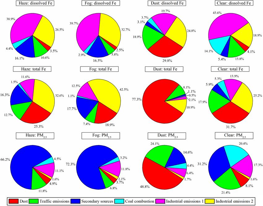
2192                                     Y. Zhu et al.: Sources and processes of iron aerosols in a megacity in Eastern China

1   Introduction                                                      undissolved to a dissolved form, thereby increasing Fe sol-
                                                                      ubility (Li et al., 2017; G. Zhang et al., 2019; Yang et al.,
The deposition of atmospheric aerosols is a major external            2020; Wong et al., 2020).
source of iron (Fe) in the ocean (Li et al., 2017; Pinedo-               The two major contributors mentioned above (aerosol pri-
González et al., 2020; Yang et al., 2020). Fe is an essential         mary sources and atmospheric acidification processes) to Fe
micronutrient that can impact phytoplankton primary pro-              solubility are associated with weather conditions, which can
ductivity, thereby modulating marine ecosystems, global car-          change the dispersion efficiency (such as boundary layer
bon cycling, and climate (Jickells et al., 2005; Tagliabue et         height, wind, and convection), dry/wet deposition and the
al., 2017; Matsui et al., 2018; Lei et al., 2018). In addition, at-   chemical conversion loss rate (Leibensperger et al., 2008;
mospheric Fe-containing particles have an adverse effect on           Zhang et al., 2018), temperature, relative humidity, and solar
human health, by generating reactive oxygen species (ROS;             radiation (Camalier et al., 2007). Recently, Shi et al. (2020)
Abbaspour et al., 2014), and can convert S(IV) to S(VI)               found that different levels of Fe solubility are closely re-
by catalytic oxidation for atmospheric sulfate (SO2−      4 ) pro-    lated with different weather conditions in one coastal city.
duction (Alexander et al., 2009). These roles of Fe largely           However, to our knowledge, studies that have attempted to
depend on the atmospheric Fe solubility (Shi et al., 2012;            investigate Fe solubility under different weather conditions
Baker et al., 2021). Unfortunately, field observations on at-         in the megacity are still sparse in the world, even though
mospheric Fe solubility are still limited, and the available          the sources of aerosol Fe (such as coal combustion, vehicle
data show a wide range of Fe solubility (0.02 % to 98 %) in           emissions, and industry emissions) are densely distributed
different atmospheric environments (Schroth et al., 2009; Shi         in megacities (Q. Zhang et al., 2019). Therefore, to better
et al., 2012; Oakes et al., 2012; Myriokefalitakis et al., 2015).     understand how aerosol primary sources and atmospheric
   There are two major processes that can significantly               acidification processing influence Fe solubility in the megac-
increase Fe solubility in atmospheric aerosols, including             ity, the planned studies should be conducted under different
aerosol primary emissions and atmospheric acidification pro-          weather conditions.
cesses (Shi et al., 2012). Dissolved Fe can be derived from              In this study, we collected atmospheric fine particles
natural and anthropogenic sources, such as mineral dust, fos-         (PM2.5 ) and individual particle samples on haze, fog, dust,
sil fuel combustion, biomass burning, and traffic exhaust             clear, and rain days at Hangzhou, a megacity of the Yangtze
(Chen et al., 2012; Pant et al., 2015; Conway et al., 2019;           River Delta (YRD), which is one of the largest modern
Rathod et al., 2020; Ito et al., 2020). Although natural emis-        megacity clusters in China. This study characterized Fe con-
sions have a high emission flux, their contribution to Fe             tent and solubility under haze, fog, dust, clear, and rain
solubility is less than 1 % (Schroth et al., 2009). Recent            weather conditions and discussed the impacts of primary
studies have highlighted anthropogenic sources due to their           sources and atmospheric acidification processes on Fe sol-
high contribution to Fe solubility. For example, Schroth et           ubility.
al. (2009) suggested that Fe solubility was less than 1 % of
the iron in arid soils, while oil combustion emissions had
                                                                      2     Methodology
a pronounced effect on Fe solubility (77 %–81 %); Oakes
et al. (2012) studied Fe solubility in anthropogenic source           2.1    Sampling site
emission samples and found that Fe solubility was 0.06 %
in coal fly, 46 % in biomass burning, 51 % in diesel exhaust,         The sampling site was located on the Zijingang Campus of
and 75 % in gasoline exhaust. These results imply that an in-         the Zhejiang University in Hangzhou (120◦ 120 E, 30◦ 160 N),
crease in relative amounts of aerosols from these mixed an-           a megacity in the YRD, China (Fig. S1 in the Supplement).
thropogenic sources may be responsible for the increase in            Industrial emissions are relatively low in Hangzhou in com-
Fe solubility.                                                        parison to other megacities in China, but traffic emissions are
   There are a number of atmospheric processes which can              serious (Xu et al., 2020). In addition, pollutants emitted in
affect Fe solubility in atmospheric aerosol particles. One of         surrounding regions and northern China can be transported
the most important processes is the mobilization of Fe in an          to Hangzhou city (Liu et al., 2021b).
acidic solution on the surface of aerosol particles because
acidic pH can trigger faster Fe dissolution and increase Fe           2.2    Sample collection
solubility (Shi et al., 2011; Maters et al., 2017; Li et al., 2017;
Zhou et al., 2020). When ambient relative humidity (RH) is            PM2.5 aerosol and individual particle samples were collected
above 60 %, aerosol particles can take up water and change            under haze, fog, dust, clear, and rain weather conditions be-
the surface to a wet or liquid state (with liquid–liquid sepa-        tween November 2018 and January 2020. Details on the sam-
ration or a homogenous state, depending on the composition            pling periods are shown in Table S1. The definitions of haze,
and RH; Sun et al., 2018; Liu et al., 2017). The wet or liquid        fog, dust, clear, and rain weather conditions are shown in
surface can take up acid gases (such as SO2 and NO2 ) and             Table S2. When the duration of haze, fog, or dust exceeded
form acidic salts to promote the conversion of Fe from an             70 % of the collection time of a sample, the sample was clas-

Atmos. Chem. Phys., 22, 2191–2202, 2022                                                https://doi.org/10.5194/acp-22-2191-2022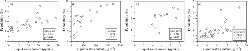
Y. Zhu et al.: Sources and processes of iron aerosols in a megacity in Eastern China                                        2193

sified as a haze, fog, or dust sample. In total, there were 34   was no significant contribution of blank subtraction to the
haze samples, 17 fog samples, 12 dust samples, 37 clear sam-     observed concentrations. The elemental concentrations used
ples, and 9 rain samples in this study.                          in this study were corrected by subtracting the filter blank
    A Th-16a intelligent sampler (Wuhan Tianhong Environ-        values.
mental Protection Industry Co., Ltd., China) with a flow rate
of 100 L min−1 was used to collect PM2.5 samples on 90 mm        2.4   Sample preparation and analysis of dissolved Fe
diameter quartz filters for 11.5 h (daytime is 08:30–20:00 lo-
cal time (LT); nighttime is 20:30–08:00 LT of the next day).     Chemical analysis of the dissolved Fe was conducted using
The sampler was installed on the rooftop of a four-story         the ferrozine technique described by Viollier et al. (2000).
teaching building (approximately 20 m above the ground)          Sample extraction and analysis were on the basis of Majes-
on the Zijingang campus of Zhejiang University. All quartz       tic et al. (2006) and Oakes et al. (2012). We conducted the
filters were firstly baked at 600 ◦ C in a muffle furnace for    analysis as follows: (1) half of the sample filters were placed
4 h to remove contaminants. Then, these filters were condi-      in clean tubes with 20 mL ammonium acetate (0.5 mM;
tioned in a room with a temperature of 20 ± 1 ◦ C and RH         pH = 4.3). Then, the tubes were placed in an ultrasonic bath
of 50 ± 2 %. After 24 h, these filters were weighed using a      for 60 min. The extractions were filtered through a 0.22 µm
Sartorius analytical balance (detection limit 0.001 mg). Af-     PTFE syringe filter to remove undissolved particles. (2) The
ter sample collection, the loaded filters were similarly con-    concentrated HCl was immediately added to the filtrate to ad-
ditioned and weighed in order to determine the PM2.5 mass        just pH equal to about 1, and then the filtrate was stored in the
concentrations. Daytime and nighttime blank samples were         refrigerator. (3) Before starting to analyze the stored solution,
collected by the same method with real samples but without       a solution of 0.01 M ascorbic acid was added to the filtrate to
operating the sampler. The collected filters were preserved in   reduce Fe(III) to Fe(II) and held for 30 min to ensure com-
a freezer at −4 ◦ C until further analysis.                      plete Fe reduction. (4) 0.01 M ferrozine solution was added
    Individual particle samples were collected four times, at    to the filtrate. (5) Ammonium acetate buffer (pH = 9.5) was
08:00, 12:00, 18:00 and 00:00 LT, on sampling days, ex-          added to the filtrate, making the pH between 4 and 9. Light
cept for rain days. The sampler is a single-stage cascade        absorption of the mixture was immediately measured by an
impactor with a 0.5 mm diameter jet nozzle and a flow rate       ultraviolet–visible spectrophotometer at 562 nm (max light
of 1.0 L min−1 . The samples were collected on copper grids      absorption of Fe(II)-Ferrozine complex) and 700 nm (back-
coated with carbon film. According to weather and visibility,    ground measurement) to yield dissolved Fe measurement.
the sampling duration spanned 30 s to 8 min. The collection      SigmaUltra-grade ammonium Fe(II) sulfate was used for
efficiency is 50 % for particles with an aerodynamic diame-      Fe(II) standards. The concentration of Fe(II) obtained from
ter of 0.1 µm and a density of 2 g cm−3 . After sampling, the    the standard curve was the concentration of dissolved Fe. The
grids were placed in a dry plastic tube and stored in a desic-   detection limit of the method for Fe(II) was 0.11 ng m−3 , cal-
cator at 25 ◦ C and 20 ± 3 % RH to minimize the exposure to      culated as 3 times the standard deviation of filter blank values
ambient air.                                                     (n = 9). The concentrations of Fe(II) in the field blanks were
                                                                 all below the detection limit, and the data reported in this
2.3   Elemental analysis
                                                                 study were corrected by subtracting the filter blank values.

Element concentrations were determined by an energy dis-         2.5   Individual particle analysis
persive X-ray fluorescence (EDXRF) spectrometer (Ep-
silon 4; Malvern Panalytical Ltd). In this method, element       Individual particle samples were analyzed with a JEM-
concentrations on a given elemental map were measured. The       2100 (JEOL Ltd.) transmission electron microscope (TEM)
measured values firstly divided by the elemental map area,       operated at 200 kV. Elemental composition was semi-
then multiplied by the total sample area to obtain element       quantitatively determined by an energy-dispersive X-ray
concentrations of the sample. Because quartz filter contains     spectrometer (EDS) that can detect elements heavier than
a large amount of silicon (Si), the Si measured by EDXRF         carbon (C). Copper (Cu) was excluded from the analyses
is not used in this study. Elements including Na, Mg, Al, P,     because the TEM grids are made of Cu. The relative per-
S, Cl, K, Ca, Ti, V, Cr, Mn, Fe, Co, Ni, Cu, Zn, Ga, As, Se,     centages of the elements were estimated based on the EDS
Sr, Ba, and Pb were measured. The National Institute of Stan-    spectra acquired through the INCA software (Oxford Instru-
dards and Technology (NIST) standard was used as reference       ments, Oxfordshire, UK). The distribution of aerosol parti-
material for standardizing the instrument. The analysis val-     cles on TEM grids was not homogeneous; coarser particles
ues of NIST standard are given in Table S3, showing that the     occur near the center, and finer particles are on the periphery.
relative errors between the measured and standard value for      Therefore, to be more representative, four areas were chosen
the standard samples were less than 10 %. The average ele-       from the center to the periphery of the sampling spot on each
ment concentrations of field blank samples (n = 4) were well     grid. The projected areas of individual particles were deter-
below those of the samples (Table S3), indicating that there     mined using iTEM software (Olympus Soft Imaging Solu-

https://doi.org/10.5194/acp-22-2191-2022                                         Atmos. Chem. Phys., 22, 2191–2202, 2022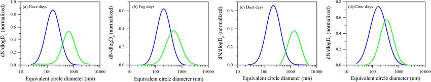
2194                                   Y. Zhu et al.: Sources and processes of iron aerosols in a megacity in Eastern China

tions GmbH, Germany), which is the standard image analysis         optimal solution. Dissolved Fe was set as total variable, and
platform for electron microscopy.                                  PM2.5 was set as a weak variable. The changes in Q values
                                                                   can provide insight into the rotation of factors. The QRobust
2.6    Water-soluble inorganic ions, organic carbon, and           (2392.94) was close to QTrue (2474.51), suggesting that PMF
       elemental carbon                                            results can reasonably explain potential sources of dissolved
                                                                   Fe.
The concentrations of water-soluble inorganic ions, includ-
                                                          2−
ing Na+ , NH+      +    2+    2+ −       −     −
              4 , K , Mg , Ca , F , Cl , NO3 , and SO4             3     Results and discussion
were obtained by an ion chromatograph (Dionex ICS-600;
Thermo Fisher Scientific). Detailed descriptions about fil-
                                                                   3.1    Pollution levels
ter extraction and analysis were given in Zhu et al. (2015).
Organic carbon (OC) and elemental carbon (EC) were ana-            The average PM2.5 concentration was the highest
lyzed by a carbon analyzer (Sunset Laboratory Inc.) with the       at 98.5 ± 19.6 µg m−3 on haze days, followed by
thermal–optical transmittance method.                              59.3 ± 11.1 µg m−3 on dust days, 56.6 ± 21.4 µg m−3
                                                                   on fog days, 33.7 ± 14.3 µg m−3 on clear days, and
2.7    Aerosol acidity and liquid water content                    24.9 ± 6.4 µg m−3 on rain days. About 100 %, 29 %, and 8 %
                                                                   of PM2.5 concentrations on haze, fog, and dust days were
A thermodynamic equilibrium model (E-AIM model II;                 higher than the grade II national PM2.5 standard of 75 µg m−3
Clegg et al., 1998) was used to calculate the aerosol acidity      (24 h average standard; GuoBiao (GB) 3095-2012, China),
(in situ acidity) and liquid water content (available at http://   respectively. However, all of PM2.5 concentrations on clear
www.aim.env.uea.ac.uk/aim/aim.php, last access: 5 Decem-           and rain days were lower than the PM2.5 grade II standard.
ber 2021). The input data include temperature, relative hu-        PM2.5 concentrations differed significantly according to the
                                            2−
midity, and the concentrations of NH+              −
                                      4 , SO4 , NO3 , and H .
                                                             +
                                                                   weather conditions (p < 0.01; independent sample T test;
                                                         2−
It was assumed that the concentration of H+ ≈ 2 × [SO4 ] +         Table S4).
[NO−            +
     3 ] − [NH4 ].
                                                                   3.2    Fe content and solubility
2.8    Positive matrix factorization (PMF)
                                                                   The average concentrations of total Fe and dissolved
The U.S. Environmental Protection Agency (U.S. EPA)                Fe were 777.6 ± 295.1 and 37.0 ± 18.4 ng m−3 on haze
PMF 5.0 model was used to identify sources of dissolved Fe         days, 929.7 ± 412.7 and 59.1 ± 38.2 ng m−3 on fog days,
and total Fe. A detailed description about PMF 5.0 is given        2945.9 ± 735.1 and 57.4 ± 12.4 ng m−3 on dust days,
in the user manual (Norris et al., 2014). There are two input      639.6 ± 195.7 and 12.8 ± 8.9 ng m−3 on clear days, and
files required to initiate the model, where one contains the       652.5 ± 306.5 and 5.4 ± 4.3 ng m−3 on rain days (Fig. 1a and
concentration values and one contains the uncertainty val-         b). Total Fe concentrations differed significantly according to
ues for each species. Uncertainty was determined as follows        the weather conditions (p < 0.01 or 0.05; independent sam-
(Polissar et al., 1998):                                           ple T test; Table S4), except between haze and clear days
                                                                   (p > 0.1) and between fog and clear days (p > 0.5). Dis-
                         5                                         solved Fe concentrations differed significantly according to
If Ci ≤ MDL,     Unc =     × MDL,                           (1)
                         6                                         weather conditions (p < 0.01 or 0.05). The contributions of
If Ci > MDL,                                                       total and dissolved Fe concentrations to PM2.5 concentra-
    p
Unc (error fraction × concentration)2 + (0.5 × MDL)2 ,      (2)    tion are shown in Table 1. The contribution of total Fe to
                                                                   PM2.5 was the largest on dust days (5.2 %), followed by rain
where Ci is the concentration value, MDL is the method de-         (2.8 %), clear (2.2 %), fog (2.0 %), and haze (0.8 %) days.
tection limit, and Unc is the uncertainty. The principals of       However, the contribution of dissolved Fe to PM2.5 was the
PMF running and species choice have been described in the          highest on fog days (0.12 %), followed by dust (0.10 %), haze
PMF 5.0 user manual and our previous study (Zhu et al.,            (0.04 %), clear (0.03 %), and rain (0.02 %) days.
2017). Since the number of samples should be 3 times higher           Fe solubility in aerosols was calculated as dissolved
than the number of species used in PMF, accurate PMF re-           Fe / total Fe concentration ×100 %. The average Fe sol-
sults could be obtained, so we used the sum of all samples         ubility was the largest on fog days (6.7 ± 3.0 %), which
under haze, fog, dust, and clear weather conditions to run         was about 1.4, 3.2, 3.5, and 7.4 times higher than that on
PMF model. In this study, 100 samples were used to run the         haze days (4.8 ± 1.9 %), dust days (2.1 ± 0.7 %), clear days
PMF model. PM2.5 , OC, EC, SO2−          −     +
                                 4 , NO3 , NH4 , Mg, Al, K,        (1.9 ± 1.0 %), and rain days (0.9 ± 0.5 %; Fig. 1c). Although
Ca, Ti, Cr, Mn, Co, Ni, Cu, Zn, As, Se, Sr, Ba, Pb, dissolved      the concentration of total Fe in dust days was the highest,
Fe, and undissolved Fe (= total Fe − dissolved Fe) were used       Fe solubility was lower than that in fog and haze days. Fe
for the PMF analysis, and six factors were resolved as the         solubility was extremely low in rain days, likely due to the

Atmos. Chem. Phys., 22, 2191–2202, 2022                                              https://doi.org/10.5194/acp-22-2191-2022
Y. Zhu et al.: Sources and processes of iron aerosols in a megacity in Eastern China 2195
Figure 1. The box-and-whisker plot of the concentrations of total Fe (a), dissolved Fe (b), and Fe solubility (c) under haze, fog, dust, clear,
and rain conditions. The solid circles above and below the box show the maximum and minimum values, respectively.
Table 1. Percentage contributions of total Fe and dissolved Fe concentrations to PM2.5 concentration under haze, fog, dust, clear, and rain
conditions. The maximum and minimum values are in parentheses.
Haze Fog Dust Clear Rain
Total Fe / PM2.5 0.8 ± 0.4 2.0 ± 1.4 5.2 ± 1.9 2.2 ± 0.9 2.8 ± 1.6
(0.4–2.2) (0.8–5.9) (3.3–10.7) (0.8–4.4) (1.1–6.3)
Dissolved Fe / PM2.5 0.04 ± 0.02 0.12 ± 0.09 0.10 ± 0.02 0.03 ± 0.02 0.02 ± 0.01
(0.00–0.07) (0.03–0.38) (0.07–0.13) (0.01–0.13) (0.00–0.05)
removal of aged aerosols by wet deposition. Fe solubility dif- strapping on the six-factor solution showed stable results,
fered significantly according to weather conditions (p < 0.01 with more than 95 out of 100 bootstrap mapped factors; fac-
or 0.05). tor chemical profiles between the base and the constrained
runs showed no significant difference (p > 0.05).
3.3 Factors influencing Fe solubility As shown in Fig. 2, factor 1 was identified as dust, with rel-
atively high loads of undissolved Fe, K, Ca, and Ti (Marsden
3.3.1 Sources of dissolved Fe and total Fe et al., 2019). Factor 2 was identified as a source of combus-
In order to identify the sources of dissolved Fe and total Fe, tion, considering its high loading of EC (Hou et al., 2012).
a PMF model was used to apportion their sources. PMF was Since there was no contribution of SO2− 4 and lower contribu-
run for 5 (Fig. S2), 6 (Fig. 2), and 7 (Fig. S3) factors for tions of K and dust elements (such as Ca and Ti), factor 2 was
the evaluation of factor profiles. In Fig. S2, factor 1 of the not associated with coal and biomass burning but with traf-
five-factor solution is represented by high contributions of fic emissions (such as petroleum and diesel combustion; Du
secondary inorganic ions (SO2− − + et al., 2018; Hao et al., 2019). Small contributions of traffic-
4 , NO3 , and NH4 ) and other
species from primary emissions, such as Cr, Mn, Co, Cu, Sr, related elements (such as Zn and Cu) suggested that factor 2
and Ba, indicating an unresolved mixing factor. In Fig. S3, represented non-exhaust traffic emissions (Lin et al., 2015).
factor 4 of the seven-factor solution only contains a relatively Factor 3 was represented by high loads of SO2− −
4 , NO3 , and
+
high contribution of EC and As, and this factor contributes NH4 , suggesting secondary sources (Pakkanen et al., 2001;
insignificantly to either PM2.5 or dissolved Fe, possibly sug- Yao et al., 2016). Factor 4 implied coal combustion because
gesting a split of meaningful factors, such as coal combus- it had high loads of SO2− 4 and As (Cui et al., 2019; Vedan-
tion or industrial emissions. Hence, six factors were selected tham et al., 2014). Factor 5 was characterized by high loads
as the final solution. The selection of the optimal solution of Cr, Co, Ni, Cu, Sr, Ba, and Pb, indicating industrial emis-
in PMF analysis was also based on the following evaluation sions (Cai et al., 2017; Chang et al., 2018; Liu et al., 2019;
criteria: a good correlation coefficient (r 2 ) between the ob- Rai et al., 2020). High loads of Co and Ni, a low load of EC,
served and predicted concentrations of fitting species, which and no OC indicated heavy oil refinery processes (Zhang et
were mostly in the range of 0.70–0.99 in this work; boot- al., 2007; Rao et al., 2012; Guo et al., 2016; Yeletsky et al.,
https://doi.org/10.5194/acp-22-2191-2022 Atmos. Chem. Phys., 22, 2191–2202, 20222196 Y. Zhu et al.: Sources and processes of iron aerosols in a megacity in Eastern China
explain why the contribution of traffic emissions to dissolved
Fe is relatively low.
Figure 3 also shows that, although industrial emissions
(factors 5 and 6 or industrial emissions 1 and industrial emis-
sions 2) contributed less than 20 % to PM2.5 on haze, fog,
dust, and clear days, they were the largest contributor to dis-
solved Fe on haze (65.4 %), fog (72.4 %), dust (44.5 %), and
clear (62.5 %) days, and they were also the largest contrib-
utor to total Fe on haze (44.2 %), fog (55.0 %), and clear
(39.1 %) days (with the exception of dust days). Industrial
emissions 1 (factor 5) similarly contributed to dissolved Fe,
regardless of the weather conditions (38.9 % to 43.6 %; with
the exception of dust days), while it only contributed 11.6 %
to 13.9 % to total Fe (with the exception of dust days). Heavy
oil-combustion-related aerosols have the highest Fe solubil-
ity (up to 78 %) from all major Fe aerosol sources (Schroth et
al., 2009; Ito et al., 2021). This may explain the much larger
contribution of industrial emissions 1 to dissolved Fe than
total Fe. Rathod et al. (2020) suggested that metal smelting
is a dominant source of anthropogenic Fe emissions. Lim-
ited data are available on the Fe solubility in particles from
metal smelting measured in high-purity water (as we did in
this paper), but Mulholland et al. (2021) showed that the Fe
solubility of industrial ash from an Fe–Mn alloy metallurgi-
cal plant is only about 2.8 % after 60 min at pH = 2 synthetic
solutions, suggesting a very low Fe solubility in the parti-
cles. Thus, it is unlikely that primary emissions of dissolved
Fe from industrial emissions 2 (factor 6) can explain its large
contribution to dissolved Fe. Furthermore, PMF results in-
dicated that secondary sources were the largest contributor
to PM2.5 on haze (66.2 %), fog (72.3 %), and clear (31.2 %)
days (with the exception of dust days). However, the contri-
bution of secondary sources to dissolved Fe was relatively
Figure 2. Factor profiles deduced from the PMF model analysis.
low, with 16.1 % on haze days, 16.5 % on fog days, 3.1 % on
dust days, and 5.4 % on clear days.
The likely reason for the high contribution of industrial
2020). Similar to factor 5, factor 6 was also observed with emissions 2 and the relatively low contribution of secondary
high loads of Cr, Cu, and Pb, but it also had high contri- sources to dissolved Fe is that PMF is unable to completely
butions of Mn, Zn, and Se. Since factors 5 and 6 were not separate secondary sources of dissolved Fe (i.e., dissolved
correlated in both time series and concentrations (Figs. S4 from insoluble Fe due to atmospheric processing) from pri-
and S5), they represented two different industrial emissions. mary sources. This means that some of the dissolved Fe due
Mn, Zn, and Pb are representative elements for steel industry to atmospheric processing may still be assigned to its primary
sources (Okuda et al., 2004; Chang et al., 2018); thus, factor factors if there is a strong co-variation between the dissolved
6 was associated with steel industry emissions. Fe and primary tracers. This suggests that the contribution
As shown in Fig. 3, traffic emissions contributed 10.6 %, of secondary sources to dissolved Fe is likely higher than
5.8 %, 18.9 %, and 13.8 % to dissolved Fe and 12.7 %, 7.4 %, that indicated by the PMF. It should also be noted that indus-
8.1 %, and 17.9 % to total Fe on haze, fog, dust, and clear trial emissions are outside the city, and thus, particles from
days, respectively. Although Fe solubility is as high as 51 % these sources undergo long-range transport before reaching
in diesel exhaust and 75 % in gasoline exhaust (Oakes et al., the sampling site. This provides more time for chemical pro-
2012), total Fe content from engine exhaust particles is ex- cessing in the atmosphere, leading to Fe solubilization. In
tremely low. It is more than likely that traffic emissions asso- the following, we further investigated the mixing of acidic
ciated with non-exhaust particles have relatively low Fe sol- species and Fe aerosols to provide further evidence for Fe
ubility. Since traffic emissions are urban sources, which are solubilization from primary insoluble Fe aerosols.
closer to the sampling site, there is less time for them to be
chemically processed in the atmosphere. These results may
Atmos. Chem. Phys., 22, 2191–2202, 2022 https://doi.org/10.5194/acp-22-2191-2022Y. Zhu et al.: Sources and processes of iron aerosols in a megacity in Eastern China 2197
Figure 3. Contributions of identified sources to dissolved Fe, total Fe, and PM2.5 on haze, fog, dust, and clear days by the PMF model.
3.3.2 Atmospheric acidification processing Fe particles (Fig. 4). This is similar to that reported by Li
et al. (2017), who confirmed that such Fe was presented as
A number of studies have considered atmospheric acidifica- Fe sulfate from nanoscale secondary ion mass spectrometry
tion processing as being a key factor influencing Fe solubil- (NanoSIMS) observations, indicative of acid dissolution. It
ity, in addition to direct emission of dissolved Fe from pri- should be noted that individual secondary sulfate particles in
mary sources (Ito and Shi, 2016; Li et al., 2017; G. Zhang et urban air normally contain nitrate, which has been confirmed
al., 2019; Shi et al., 2020; Zhu et al., 2020; Liu et al., 2021a). in single particle mass spectrometry studies (Whiteaker et al.,
As mentioned above, a proportion of dissolved Fe was as- 2002; Li et al., 2016).
sociated with a PMF factor identified as secondary sources We further calculated the number contribution of S-Fe par-
during haze, fog, dust, and clear days, thereby suggesting ticles to Fe-containing particles, with 76.3 % on haze days,
a contribution from atmospheric processing. To further sup- 87.1 % on fog days, 78.3 % on dust days, and 81.8 % on clear
port this result, a total of 688, 404, 580, and 311 individ- days. The result suggested that Fe particles were mostly in-
ual particles on haze, fog, dust, and clear days were ana- ternally mixed with acidic secondary aerosol species. To fur-
lyzed by TEM/EDS, respectively. On rain days, individual ther investigate the impact of aerosol acidification on Fe sol-
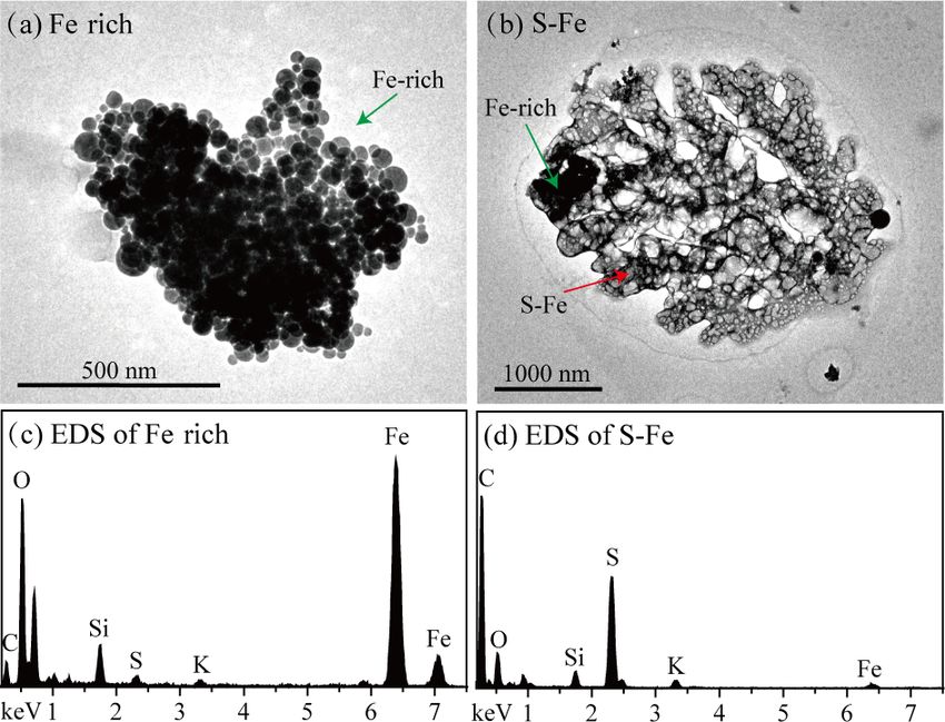
particle samples were not collected. TEM analysis showed ubility, the correlation of aerosol acidity/total Fe with Fe sol-
two types of Fe-containing particles, i.e., Fe-rich and S-Fe ubility was calculated. Aerosol acidity was estimated by the
particles. Figure 4 shows that Fe-rich particles usually con- E-AIM model. As shown in Fig. 5, aerosol acidity/total Fe
tain aggregates of multiple spherical Fe particles. TEM/EDS and Fe solubility show a good correlation on fog (r = 0.85,
also detected minor Fe, besides major elements (S, C, and p < 0.01), haze (r = 0.56, p < 0.01), and clear (r = 0.53,
O), in acidic secondary aerosols, and these were named S-
https://doi.org/10.5194/acp-22-2191-2022 Atmos. Chem. Phys., 22, 2191–2202, 20222198 Y. Zhu et al.: Sources and processes of iron aerosols in a megacity in Eastern China
79 % and 47 %–78 %, respectively. When RH > 60 %, aver-
age aerosol acidity/total Fe was 2.3 and 2.1 µmol µmol−1 on
haze and clear days, respectively, and similar to that on fog
days (2.4 µmol µmol−1 ). However, Fe solubility on haze and
clear days at 5.7 % and 2.6 % were lower than 6.7 % on fog
days. This could be due to the low RH on haze and clear days,
which led to lower water content on the particles relative to
fog days. The low water content in the aerosol particles may
have limited the uptake and oxidation of acidic gases. When
RH < 60 %, Fe solubility on haze and clear days was lower
than 3.9 % and 2.3 %, respectively, even when aerosol acid-
ity/total Fe was high. On dust days, RH only ranged from
22 % to 48 % and Fe solubility was less than 2.9 %. Further-
more, the E-AIM model was also employed to estimate liquid
water content. Lower correlations between the Fe solubility
and liquid water content on haze (r = 0.74; p < 0.01), clear
Figure 4. Typical TEM images and corresponding EDS spectra
(r = 0.65; p < 0.01), and dust (r = 0.58; p < 0.05) days than
of Fe-rich and S-Fe particles. (a) TEM image of Fe-rich parti- on fog days (r = 0.79; p < 0.01) further supported these re-
cles. (b) TEM image of S-Fe particles. (c) EDS of Fe-rich particle. sults (Fig. 7).
(d) EDS of S-Fe particle.
4 Summary and atmospheric implications
The average Fe solubility was the largest on fog days
(6.7 ± 3.0 %), which was about 1.4 times higher than on haze
days (4.8 ± 1.9 %), 3.2 times higher than on dust days (2.1 ±
0.7 %), 3.5 times higher than on clear days (1.9 ± 1.0 %),
and 7.4 times higher than on rain days (0.9 ± 0.5 %). Indus-
trial emissions were the largest contributor to dissolved Fe
(44.5 %–72.4 %) and total Fe (39.1 %–55.0 %; with the ex-
ception of dust days) during haze, fog, dust, and clear condi-
tions. Although small on dust (3.1 %) and clear (5.4 %) days,
secondary sources significantly contributed to dissolved Fe
on haze (16.1 %) and fog (16.5 %) days. Individual particle
analysis further showed that about 76.3 %, 87.1 %, 78.3 %,
and 81.8 % of Fe-containing particles were internally mixed
Figure 5. Correlations between Fe solubility and aerosol acidity or
with acidic secondary aerosol particles under haze, fog, dust,
total Fe under different RH. and clear conditions, respectively. Our study indicated that
the wet surface of aerosol particles (when RH > 60 %) may
facilitate the update of acidic species and, thereby, promote
p < 0.01) days (with the exception of dust days). These re- Fe dissolution and increase Fe solubility. Higher RH on
sults further supported the above argument that the solubi- fog days (> 90 %) compared with haze (35 %–79 %), dust
lization of Fe aerosols by acids. In addition, Fig. 6 shows (22 %–48 %), and clear (47 %–78 %) days resulted in more
that acidic secondary aerosol species (e.g., sulfate and ni- effective aerosol acidification and higher Fe solubility.
trate) increase the size of Fe particles by about 3.6, 2.4, 4.7, Maher et al. (2016) and Lu et al. (2020) reported that,
and 1.9 times under haze, fog, dust, and clear conditions, re- when the atmospheric Fe3 O4 particle has a size of < 200 nm,
spectively. it can access the brain directly via transport through the neu-
On the other hand, particles with a wet surface can eas- ronal axons of the olfactory or trigeminal nerves. In this
ily take up acidic gases (such as SO2 and NO2 ) to produce study, the peak size of Fe-rich particles was 175, 200, 225,
acidic salts (such as sulfate and nitrate), which can promote and 175 nm on haze, fog, dust, and clear days, respectively.
Fe dissolution (Wang et al., 2019; Li et al., 2017, 2021). Un- Therefore, Fe aerosols, regardless of the weather conditions,
der fog conditions, the RH was higher than 90 %, which was are a potential hazard to human health in densely populated
much higher than the threshold (60 %) of the particle sur- megacities.
face changed to a wet or liquid state (Sun et al., 2018; Liu et Fe-containing particles from the continent can be trans-
al., 2017). On haze and clear days, RH ranged from 35 %– ported and further deposited to the ocean (Winton et al.,
Atmos. Chem. Phys., 22, 2191–2202, 2022 https://doi.org/10.5194/acp-22-2191-2022Y. Zhu et al.: Sources and processes of iron aerosols in a megacity in Eastern China 2199
Figure 6. Size distributions of Fe-rich (blue line) and S-Fe (green line) particles under haze (a), fog (b), dust (c), and clear (d) conditions.
The size of the S-Fe particles represents the dry state of individual particles on the substrate. The distribution pattern is normalized.
Figure 7. Correlations between Fe solubility and liquid water content on haze (a), fog (b), dust (c), and clear (d) days.
2015; Yoshida et al., 2018; Conway et al., 2019). Li et Disclaimer. Publisher’s note: Copernicus Publications remains
al. (2017) found large amounts of anthropogenic fine Fe- neutral with regard to jurisdictional claims in published maps and
containing particles in the East China Sea. In this study, the institutional affiliations.
prevailing winds during the sampling period were dominated
by the westerly or northwesterly winds under haze, fog, and
dust conditions, suggesting that Fe-containing particles were Acknowledgements. We thank the Atmospheric Science Prac-
likely transported into the ocean. In the future, biogeochemi- tice Center of the School of Earth Sciences, Zhejiang University,
for sharing the meteorological data during the sampling period.
cal cycle model should consider Fe-containing particles from
upwind continental areas of the ocean.
Financial support. This research has been supported by the Na-
tional Natural Science Foundation of China (grant nos. 41907186
Data availability. The data used in this study are available from
and 42075096), the China Postdoctoral Science Foundation (grant
the corresponding author upon request (liweijun@zju.edu.cn).
no. 2019M652059), the Natural Science Foundation of Zhe-
jiang Province (grant no. LZ19D050001), and the UK Natural
Environment Research Council (grant nos. NE/N007190/1 and
Supplement. The supplement related to this article is available NE/R005281/1).
online at: https://doi.org/10.5194/acp-22-2191-2022-supplement.
Review statement. This paper was edited by Timothy Bertram
Author contributions. YZ, WL, and ZS designed the study. JZ, and reviewed by two anonymous referees.
YZ, LL, and LX collected aerosol and individual particle samples.
YZ and YW contributed the laboratory experiments. YZ, WL, ZS,
and JX performed the data analysis. YZ and WL wrote the paper and
prepared the material, with contributions from all the co-authors. JS, References
LS, PF, DZ and ZS commented on the paper.
Abbaspour, N., Hurrell, R., and Kelishadi, R.: Review on iron and
its importance for human health, J. Res. Med. Sci., 19, 164–174,
Competing interests. The contact author has declared that nei- 2014.
ther they nor their co-authors have any competing interests. Alexander, B., Park, R. J., Jacob, D. J., and Gong, S.: Transition
metal-catalyzed oxidation of atmospheric sulfur: global impli-
cations for the sulfur budget, J. Geophys. Res.-Atmos., 114,
D02309, https://doi.org/10.1029/2008JD010486, 2009.
https://doi.org/10.5194/acp-22-2191-2022 Atmos. Chem. Phys., 22, 2191–2202, 20222200 Y. Zhu et al.: Sources and processes of iron aerosols in a megacity in Eastern China
Baker, A., Kanakidou, M., Nenes, A., Myriokefalitakis, S., Croot, Ito, A. and Shi, Z.: Delivery of anthropogenic bioavailable iron
P. L., Duce, R. A., Gao, Y., Guieu, C., Ito, A., Jickells, T., Ma- from mineral dust and combustion aerosols to the ocean, At-
howald, N. M., Middag, R., Perron, M. M. G., Sarin, M. M., mos. Chem. Phys., 16, 85–99, https://doi.org/10.5194/acp-16-85-
Shelley, R., and Turner, D. R.: Changing atmospheric acidity as 2016, 2016.
a modulator of nutrient deposition and ocean biogeochemistry, Ito, A., Perron, M. M., Proemse, B. C., Strzelec, M., Gault-Ringold,
Sci. Adv., 7, eabd8800, https://doi.org/10.1126/sciadv.abd8800, M., Boyd, P. W., and Bowie, A. R.: Evaluation of aerosol iron
2021. solubility over Australian coastal regions based on inverse mod-
Cai, J., Wang, J., Zhang, Y., Tian, H., Zhu, C., Gross, D. eling: implications of bushfires on bioaccessible iron concentra-
S., Hu, M., Hao, J., He, K., Wang, S., and Zheng, M.: tions in the Southern Hemisphere, Prog. Earth Planet. Sc., 7, 1–
Source apportionment of Pb-containing particles in Bei- 17, https://doi.org/10.1186/s40645-020-00357-9, 2020.
jing during January 2013, Environ. Pollut., 226, 30–40, Ito, A., Ye, Y., Baldo, C., and Shi, Z. B.: Ocean fertiliza-
https://doi.org/10.1016/j.envpol.2017.04.004, 2017. tion by pyrogenic aerosol iron, npj Clim. Atmos. Sci., 4, 30,
Camalier, L., Cox, W., and Dolwick, P.: The effects of meteorol- https://doi.org/10.1038/s41612-021-00185-8, 2021.
ogy and their use in assessing ozone trends, Atmos. Environ., 41, Jickells, T., An, Z., Andersen, K. K., Baker, A., Berga-
7127–7137, 2007. metti, G., Brooks, N., Cao, J., Boyd, P., Duce, R., and
Chang, Y., Huang, K., Xie, M., Deng, C., Zou, Z., Liu, S., and Hunter, K.: Global iron connections between desert dust,
Zhang, Y.: First long-term and near real-time measurement of ocean biogeochemistry, and climate, Science, 308, 67–71,
trace elements in China’s urban atmosphere: temporal variabil- https://doi.org/10.1126/science.1105959, 2005.
ity, source apportionment and precipitation effect, Atmos. Chem. Lei, C., Sun, Y., Tsang, D. C. W., and Lin, D.: Envi-
Phys., 18, 11793–11812, https://doi.org/10.5194/acp-18-11793- ronmental transformations and ecological effects of
2018, 2018. iron-based nanoparticles, Environ. Pollut., 232, 10–30,
Chen, H., Laskin, A., Baltrusaitis, J., Gorski, C. A., Scherer, M. https://doi.org/10.1016/j.envpol.2017.09.052, 2018.
M., and Grassian, V. H.: Coal Fly Ash as a Source of Iron Leibensperger, E. M., Mickley, L. J., and Jacob, D. J.: Sensitivity
in Atmospheric Dust, Environ. Sci. Technol., 46, 2112–2120, of US air quality to mid-latitude cyclone frequency and impli-
https://doi.org/10.1021/es204102f, 2012. cations of 1980–2006 climate change, Atmos. Chem. Phys., 8,
Clegg, S. L., Brimblecombe, P., and Wexler, A. S.: Thermody- 7075–7086, https://doi.org/10.5194/acp-8-7075-2008, 2008.
2−
namic model of the system H+ -NH+ −
4 -SO4 -NO3 -H2 O at tro- Li, W., Sun, J., Xu, L., Shi, Z., Riemer, N., Sun, Y., Fu, P., Zhang, J.,
pospheric temperatures, J. Phys. Chem. A, 102, 2137–2154, Lin, Y., and Wang, X.: A conceptual framework for mixing struc-
https://doi.org/10.1021/jp973042r, 1998. tures in individual aerosol particles, J. Geophys. Res.-Atmos.,
Conway, T. M., Hamilton, D. S., Shelley, R. U., Aguilar-Islas, A. 121, 13784–13798, https://doi.org/10.1002/2016JD025252,
M., Landing, W. M., Mahowald, N. M., and John, S. G.: Tracing 2016.
and constraining anthropogenic aerosol iron fluxes to the North Li, W., Xu, L., Liu, X., Zhang, J., Lin, Y., Yao, X., Gao, H., Zhang,
Atlantic Ocean using iron isotopes, Nat. Commun., 10, 1–10, D., Chen, J., and Wang, W.: Air pollution–aerosol interactions
https://doi.org/10.1038/s41467-019-10457-w, 2019. produce more bioavailable iron for ocean ecosystems, Sci. Adv.,
Cui, Y., Ji, D., Chen, H., Gao, M., Maenhaut, W., He, 3, e1601749, https://doi.org/10.1126/sciadv.1601749, 2017.
J., and Wang, Y.: Characteristics and Sources of Hourly Li, W., Teng, X., Chen, X., Liu, L., Xu, L., Zhang, J.,
Trace Elements in Airborne Fine Particles in Urban Bei- Wang, Y., Zhang, Y., and Shi, Z.: Organic Coating Re-
jing, China, J. Geophys. Res.-Atmos., 124, 11595–11613, duces Hygroscopic Growth of Phase-Separated Aerosol
https://doi.org/10.1029/2019jd030881, 2019. Particles, Environ. Sci. Technol., 55, 16339–16346,
Du, Z., Hu, M., Peng, J., Zhang, W., Zheng, J., Gu, F., Qin, Y., https://doi.org/10.1021/acs.est.1c05901, 2021.
Yang, Y., Li, M., Wu, Y., Shao, M., and Shuai, S.: Compari- Lin, Y.-C., Tsai, C.-J., Wu, Y.-C., Zhang, R., Chi, K.-H., Huang,
son of primary aerosol emission and secondary aerosol formation Y.-T., Lin, S.-H., and Hsu, S.-C.: Characteristics of trace met-
from gasoline direct injection and port fuel injection vehicles, At- als in traffic-derived particles in Hsuehshan Tunnel, Taiwan: size
mos. Chem. Phys., 18, 9011–9023, https://doi.org/10.5194/acp- distribution, potential source, and fingerprinting metal ratio, At-
18-9011-2018, 2018. mos. Chem. Phys., 15, 4117–4130, https://doi.org/10.5194/acp-
Guo, K., Li, H., and Yu, Z.: In-situ heavy and extra- 15-4117-2015, 2015.
heavy oil recovery: A review, Fuel, 185, 886–902, Liu, L., Lin, Q. H., Liang, Z., Du, R. G., Zhang, G. Z., Zhu, Y.
https://doi.org/10.1016/j.fuel.2016.08.047, 2016. H., Qi, B.; Zhou, S. Z., and Li, W. J.: Variations in concentra-
Hao, Y., Gao, C., Deng, S., Yuan, M., Song, W., Lu, Z., tion and solubility of iron in atmospheric fine particles during the
and Qiu, Z.: Chemical characterisation of PM2.5 emitted COVID-19 pandemic: An example from China, Gondwana Res.,
from motor vehicles powered by diesel, gasoline, natural 97, 138–144, https://doi.org/10.1016/j.gr.2021.05.022, 2021a.
gas and methanol fuel, Sci. Total Environ., 674, 128–139, Liu, L., Zhang, J., Du, R., Teng, X., Hu, R., Yuan, Q., Tang, S.,
https://doi.org/10.1016/j.scitotenv.2019.03.410, 2019. Ren, C., Huang, X., Xu, L., Zhang, Y., Zhang, X., Song, C.,
Hou, L., Wang, S., Dou, C., Zhang, X., Yu, Y., Zheng, Y., Avula, U., Liu, B., Lu, G., Shi, Z., and Li, W.: Chemistry of Atmospheric
Hoxha, M., Díaz, A., McCracken, J., Barretta, F., Marinelli, B., Fine Particles During the COVID-19 Pandemic in a Megac-
Bertazzi, P. A., Schwartz, J., and Baccarelli, A. A.: Air pollution ity of Eastern China, Geophys. Res. Lett., 48, 2020GL091611,
exposure and telomere length in highly exposed subjects in Bei- https://doi.org/10.1029/2020GL091611, 2021b.
jing, China: A repeated-measure study, Environ. Int., 48, 71–77, Liu, S., Zhu, C., Tian, H., Wang, Y., Zhang, K., Wu, B.,
https://doi.org/10.1016/j.envint.2012.06.020, 2012. Liu, X., Hao, Y., Liu, W., Bai, X., Lin, S., Wu, Y., Shao,
Atmos. Chem. Phys., 22, 2191–2202, 2022 https://doi.org/10.5194/acp-22-2191-2022Y. Zhu et al.: Sources and processes of iron aerosols in a megacity in Eastern China 2201 P., and Liu, H.: Spatiotemporal Variations of Ambient Con- Okuda, T., Kato, J., Mori, J., Tenmoku, M., Suda, Y., Tanaka, centrations of Trace Elements in a Highly Polluted Re- S., He, K., Ma, Y., Yang, F., Yu, X., Duan, F., and Lei, Y.: gion of China, J. Geophys. Res.-Atmos., 124, 4186–4202, Daily concentrations of trace metals in aerosols in Beijing, https://doi.org/10.1029/2018jd029562, 2019. China, determined by using inductively coupled plasma mass Liu, Y., Wu, Z., Wang, Y., Xiao, Y., Gu, F., Zheng, J., Tan, spectrometry equipped with laser ablation analysis, and source T., Shang, D., Wu, Y., Zeng, L., Hu, M., Bateman, A. P., identification of aerosols, Sci. Total Environ., 330, 145–158, and Martin, S. T.: Submicrometer particles are in the liq- https://doi.org/10.1016/j.scitotenv.2004.04.010, 2004. uid state during heavy haze episodes in the urban atmosphere Pakkanen, T. A., Loukkola, K., Korhonen, C. H., Aurela, M., of Beijing, China, Environ. Sci. Technol. Lett., 4, 427–432, Makela, T., Hillamo, R. E., Aarnio, P., Koskentalo, T., Kousa, https://doi.org/10.1021/acs.estlett.7b00352, 2017. A., and Maenhaut, W.: Sources and chemical composition of Lu, D., Luo, Q., Chen, R., Zhuansun, Y., Jiang, J., Wang, W., atmospheric fine and coarse particles in the Helsinki area, At- Yang, X., Zhang, L., Liu, X., Li, F., Liu, Q., and Jiang, G.: mos. Environ., 35, 5381–5391, https://doi.org/10.1016/S1352- Chemical multi-fingerprinting of exogenous ultrafine particles 2310(01)00307-7, 2001. in human serum and pleural effusion, Nat. Commun., 11, 2567, Pant, P., Baker, S. J., Shukla, A., Maikawa, C., Pollitt, K. J. https://doi.org/10.1038/s41467-020-16427-x, 2020. G., and Harrison, R. M.: The PM10 fraction of road dust Maher, B. A., Ahmed, I. A. M., Karloukovski, V., MacLaren, D. A., in the UK and India: Characterization, source profiles and Foulds, P. G., Allsop, D., Mann, D. M. A., Torres-Jardón, R., and oxidative potential, Sci. Total Environ., 530-531, 445–452, Calderon-Garciduenas, L.: Magnetite pollution nanoparticles in https://doi.org/10.1016/j.scitotenv.2015.05.084, 2015. the human brain, P. Natl. Acad. Sci. USA, 113, 10797–10801, Pinedo-González, P., Hawco, N. J., Bundy, R. M., Armbrust, E. V., https://doi.org/10.1073/pnas.1605941113, 2016. Follows, M. J., Cael, B., White, A. E., Ferrón, S., Karl, D. M., Majestic, B. J., Schauer, J. J., Shafer, M. M., Turner, J. R., and John, S. G.: Anthropogenic Asian aerosols provide Fe to Fine, P. M., Singh, M., and Sioutas, C.: Development of the North Pacific Ocean, P. Natl. Acad. Sci. USA, 117, 27862– a wet-chemical method for the speciation of iron in at- 27868, https://doi.org/10.1073/pnas.2010315117, 2020. mospheric aerosols, Environ. Sci. Technol., 40, 2346–2351, Polissar, A. V., Hopke, P. K., Paatero, P., Malm, W. C., and Sisler, https://doi.org/10.1021/es052023p, 2006. J. F.: Atmospheric aerosol over Alaska: 2. Elemental composi- Marsden, N. A., Ullrich, R., Möhler, O., Eriksen Hammer, S., Kan- tion and sources, J. Geophys. Res.-Atmos., 103, 19045–19057, dler, K., Cui, Z., Williams, P. I., Flynn, M. J., Liu, D., Allan, J. https://doi.org/10.1029/98JD01212, 1998. D., and Coe, H.: Mineralogy and mixing state of north African Rai, P., Furger, M., Slowik, J. G., Canonaco, F., Fröhlich, R., mineral dust by online single-particle mass spectrometry, At- Hüglin, C., Minguillón, M. C., Petterson, K., Baltensperger, U., mos. Chem. Phys., 19, 2259–2281, https://doi.org/10.5194/acp- and Prévôt, A. S. H.: Source apportionment of highly time- 19-2259-2019, 2019. resolved elements during a firework episode from a rural free- Maters, E. C., Delmelle, P., and Gunnlaugsson, H. P.: Controls on way site in Switzerland, Atmos. Chem. Phys., 20, 1657–1674, iron mobilisation from volcanic ash at low pH: Insights from dis- https://doi.org/10.5194/acp-20-1657-2020, 2020. solution experiments and Mössbauer spectroscopy, Chem. Geol., Rao, B. P. S., Chauhan, C., Mhaisalkar, V. A., Kumar, A., De- 449, 73–81, https://doi.org/10.1016/j.chemgeo.2016.11.036, votta, S., and Wate, S. R.: Factor Analysis for Estimating Source 2017. Contribution to Ambient Airborne Particles in and Around a Matsui, H., Mahowald, N. M., Moteki, N., Hamilton, D. S., Ohata, Petroleum Refinery in India, Indian Chem. Eng., 54, 12–21, S., Yoshida, A., Koike, M., Scanza, R. A., and Flanner, M. G.: https://doi.org/10.1080/00194506.2012.714138, 2012. Anthropogenic combustion iron as a complex climate forcer, Nat. Rathod, S. D., Hamilton, D., Mahowald, N., Klimont, Z., Cor- Commun., 9, 1–10, https://doi.org/10.1038/s41467-018-03997- bett, J., and Bond, T.: A Mineralogy-Based Anthropogenic 0, 2018. Combustion-Iron Emission Inventory, J. Geophys. Res.-Atmos., Mulholland, D. S., Flament, P., de Jong, J., Mattielli, N., Deboudt, 125, e2019JD032114, https://doi.org/10.1029/2019JD032114, K., Dhont, G., and Bychkov, E.: In-cloud processing as a possi- 2020. ble source of isotopically light iron from anthropogenic aerosols: Schroth, A. W., Crusius, J., Sholkovitz, E. R., and Bostick, B. C.: New insights from a laboratory study, Atmos. Environ., 259, Iron solubility driven by speciation in dust sources to the ocean, 118505, https://doi.org/10.1016/j.atmosenv.2021.118505, 2021. Nat. Geosci., 2, 337–340, https://doi.org/10.1038/ngeo501, Myriokefalitakis, S., Daskalakis, N., Mihalopoulos, N., Baker, 2009. A. R., Nenes, A., and Kanakidou, M.: Changes in dissolved Shi, J., Guan, Y., Ito, A., Gao, H., Yao, X., Baker, A. R., and iron deposition to the oceans driven by human activity: a Zhang, D.: High production of soluble iron promoted by aerosol 3-D global modelling study, Biogeosciences, 12, 3973–3992, acidification in fog, Geophys. Res. Lett., 47, e2019GL086124, https://doi.org/10.5194/bg-12-3973-2015, 2015. https://doi.org/10.1029/2019GL086124, 2020. Norris, G., Duvall, R., Brown, S., and Bai, S.: EPA positive matrix Shi, Z., Krom, M. D., Bonneville, S., Baker, A. R., Bristow, C., factorization (PMF) 5.0 fundamentals and user guide, US Envi- Drake, N., Mann, G., Carslaw, K., McQuaid, J. B., Jickells, T., ronmental Protection Agency, 1-136, EPA/600/R-14/108, 2014. and Benning, L. G.: Influence of chemical weathering and aging Oakes, M., Ingall, E., Lai, B., Shafer, M., Hays, M., Liu, Z., Russell, of iron oxides on the potential iron solubility of Saharan dust A., and Weber, R.: Iron solubility related to particle sulfur con- during simulated atmospheric processing, Global Biogeochem. tent in source emission and ambient fine particles, Environ. Sci. Cy., 25, GB2010, https://doi.org/10.1029/2010GB003837, 2011. Technol., 46, 6637–6644, https://doi.org/10.1021/es300701c, Shi, Z., Krom, M. D., Jickells, T. D., Bonneville, S., Carslaw, K. 2012. S., Mihalopoulos, N., Baker, A. R., and Benning, L. G.: Impacts https://doi.org/10.5194/acp-22-2191-2022 Atmos. Chem. Phys., 22, 2191–2202, 2022
2202                                      Y. Zhu et al.: Sources and processes of iron aerosols in a megacity in Eastern China

  on iron solubility in the mineral dust by processes in the source     Yeletsky, P. M., Zaikina, O. O., Sosnin, G. A., and Kukushkin, R.
  region and the atmosphere: A review, Aeolian Res., 5, 21–42,            G.: Heavy oil cracking in the presence of steam and nanodis-
  https://doi.org/10.1029/2010GB003837, 2012.                             persed catalysts based on different metals, Fuel Process. Tech-
Sun, J., Liu, L., Xu, L., Wang, Y., Wu, Z., Hu, M., Shi, Z., Li, Y.,      nol., 199, 106239, https://doi.org/10.1016/j.fuproc.2019.106239,
  Zhang, X., Chen, J., and Li, W.: Key role of nitrate in phase tran-     2020.
  sitions of urban particles: implications of important reactive sur-   Yoshida, A., Ohata, S., Moteki, N., Adachi, K., Mori, T., Koike,
  faces for secondary aerosol formation, J. Geophys. Res.-Atmos.,         M., and Takami, A.: Abundance and Emission Flux of the An-
  123, 1234–1243, https://doi.org/10.1002/2017JD027264, 2018.             thropogenic Iron Oxide Aerosols From the East Asian Conti-
Tagliabue, A., Bowie, A. R., Boyd, P. W., Buck, K. N.,                    nental Outflow, J. Geophys. Res.-Atmos., 123, 11194–11209,
  Johnson, K. S., and Saito, M. A.: The integral role                     https://doi.org/10.1029/2018JD028665, 2018.
  of iron in ocean biogeochemistry, Nature, 543, 51–59,                 Zhang, G., Lin, Q., Peng, L., Yang, Y., Jiang, F., Liu, F.,
  https://doi.org/10.1038/nature21058, 2017.                              Song, W., Chen, D., Cai, Z., and Bi, X.: Oxalate for-
Vedantham, R., Landis, M. S., Olson, D., and Pancras, J. P.: Source       mation enhanced by Fe-containing particles and environ-
  Identification of PM2.5 in Steubenville, Ohio Using a Hybrid            mental implications, Environ. Sci. Technol., 53, 1269–1277,
  Method for Highly Time-Resolved Data, Environ. Sci. Technol.,           https://doi.org/10.1021/acs.est.8b05280, 2019.
  48, 1718–1726, https://doi.org/10.1021/es402704n, 2014.               Zhang, Q., Zheng, Y., Tong, D., Shao, M., Wang, S., Zhang, Y., Xu.
Viollier, E., Inglett, P., Hunter, K., Roychoudhury, A., and Van Cap-     X., Wang. J., He, H., Liu, W., Ding, Y., Lei, Y., Li, J., Wang,
  pellen, P.: The ferrozine method revisited: Fe (II)/Fe (III) de-        Z., Zhang, X., Wang, Y., Cheng, J., Liu, Y., Shi, Q., Yan, L.,
  termination in natural waters, Appl. Geochem., 15, 785–790,             Geng, G., Hong, C., Li, M., Liu, F., Zheng, B., Cao, J., Ding,
  https://doi.org/10.1016/S0883-2927(99)00097-9, 2000.                    A., Gao, J., Fu, Q., Huo, J., Liu, B., Liu, Z., Yang, F., He, K.,
Wang, Z., Wang, T., Fu, H., Zhang, L., Tang, M., George, C., Gras-        and Hao, J.: Drivers of improved PM2.5 air quality in China
  sian, V. H., and Chen, J.: Enhanced heterogeneous uptake of             from 2013 to 2017, P. Natl. Acad. Sci. USA, 116, 24463–24469,
  sulfur dioxide on mineral particles through modification of iron        https://doi.org/10.1073/pnas.1907956116, 2019.
  speciation during simulated cloud processing, Atmos. Chem.            Zhang, S., Liu, D., Deng, W., and Que, G.: A Review of Slurry-
  Phys., 19, 12569–12585, https://doi.org/10.5194/acp-19-12569-           Phase Hydrocracking Heavy Oil Technology, Energ. Fuel., 21, 6,
  2019, 2019.                                                             3057–3062, https://doi.org/10.1021/ef700253f, 2007.
Whiteaker, J. R., Suess, D. T., and Prather, K. A.: Effects of Me-      Zhang, X., Zhong, J., Wang, J., Wang, Y., and Liu, Y.: The inter-
  teorological Conditions on Aerosol Composition and Mixing               decadal worsening of weather conditions affecting aerosol pol-
  State in Bakersfield, CA, Environ. Sci. Technol., 36, 2345–2353,        lution in the Beijing area in relation to climate warming, At-
  https://doi.org/10.1021/es011381z, 2002.                                mos. Chem. Phys., 18, 5991–5999, https://doi.org/10.5194/acp-
Winton, V. H. L., Bowie, A. R., Edwards, R., Keywood,                     18-5991-2018, 2018.
  M., Townsend, A. T., van der Merwe, P., and Boll-                     Zhou, Y., Zhang, Y., Griffith, S. M., Wu, G., Li, L., Zhao,
  höfer, A.: Fractional iron solubility of atmospheric iron in-           Y., Li, M., Zhou, Z., and Yu, J. Z.: Field Evidence
  puts to the Southern Ocean, Mar. Chem., 177, 20—32,                     of Fe-Mediated Photochemical Degradation of Oxalate and
  https://doi.org/10.1016/j.marchem.2015.06.006, 2015.                    Subsequent Sulfate Formation Observed by Single Particle
Wong, J. P. S., Yang, Y., Fang, T., Mulholland, J. A., Russell,           Mass Spectrometry, Environ. Sci. Technol., 54, 6562–6574,
  A. G., Ebelt, S., Nenes, A., and Weber, R. J.: Fine Parti-              https://doi.org/10.1021/acs.est.0c00443, 2020.
  cle Iron in Soils and Road Dust Is Modulated by Coal-Fired            Zhu, Y., Yang, L., Meng, C., Yuan, Q., Yan, C., Dong, C., Sui, X.,
  Power Plant Sulfur, Environ. Sci. Technol., 54, 7088–7096,              Yao, L., Yang, F., and Lu, Y.: Indoor/outdoor relationships and
  https://doi.org/10.1021/acs.est.0c00483, 2020.                          diurnal/nocturnal variations in water-soluble ion and PAH con-
Xu, L., Zhang, J., Sun, X., Xu, S., Shan, M., Yuan, Q.,                   centrations in the atmospheric PM2.5 of a business office area in
  Liu, L., Du, Z., Liu, D., Xu, D., Song, C., Liu, B., Lu,                Jinan, a heavily polluted city in China, Atmos. Res., 153, 276–
  G., Shi, Z., and Li, W.: Variation in Concentration and                 285, https://doi.org/10.1016/j.atmosres.2014.08.014, 2015.
  Sources of Black Carbon in a Megacity of China During the             Zhu, Y., Yang, L., Kawamura, K., Chen, J., Ono, K., Wang, X.,
  COVID-19 Pandemic, Geophys. Res. Lett., 47, e2020GL090444,              Xue, L., and Wang, W.: Contributions and source identification
  https://doi.org/10.1029/2020GL090444, 2020.                             of biogenic and anthropogenic hydrocarbons to secondary or-
Yang, T., Chen, Y., Zhou, S., Li, H., Wang, F., and Zhu, Y.: Solu-        ganic aerosols at Mt. Tai in 2014, Environ. Pollut., 220, 863–872,
  bilities and deposition fluxes of atmospheric Fe and Cu over the        https://doi.org/10.1016/j.envpol.2016.10.070, 2017.
  Northwest Pacific and its marginal seas, Atmos. Environ., 239,        Zhu, Y., Li, W., Lin, Q., Yuan, Q., Liu, L., Zhang, J.,
  117763, https://doi.org/10.1016/j.atmosenv.2020.117763, 2020.           Zhang, Y., Shao, L., Niu, H., and Yang, S.: Iron sol-
Yao, L., Yang, L. X., Yuan, Q., Yan, C., Dong, C., Meng,                  ubility in fine particles associated with secondary acidic
  C. P., Sui, X., Yang, F., Lu, Y. L., and Wang, W. X.:                   aerosols in east China, Environ. Pollut., 264, 114769,
  Sources apportionment of PM2.5 in a background site in                  https://doi.org/10.1016/j.envpol.2020.114769, 2020.
  the North China Plain, Sci. Total Environ., 541, 590–598,
  https://doi.org/10.1016/j.scitotenv.2015.09.123, 2016.

Atmos. Chem. Phys., 22, 2191–2202, 2022                                                   https://doi.org/10.5194/acp-22-2191-2022
You can also read


