Still normal? Near-real-time evaluation of storm surge events in the context of climate change
←
→
Page content transcription
If your browser does not render page correctly, please read the page content below

Nat. Hazards Earth Syst. Sci., 22, 97–116, 2022
https://doi.org/10.5194/nhess-22-97-2022
© Author(s) 2022. This work is distributed under
the Creative Commons Attribution 4.0 License.

Still normal? Near-real-time evaluation of storm surge events
in the context of climate change
Xin Liu, Insa Meinke, and Ralf Weisse
Institute of Coastal Systems – Analysis and Modeling, Helmholtz-Zentrum Hereon,
Max-Planck-Str. 1, 21502 Geesthacht, Germany

Correspondence: Ralf Weisse (ralf.weisse@hereon.de)

Received: 10 March 2021 – Discussion started: 23 April 2021
Revised: 16 November 2021 – Accepted: 4 December 2021 – Published: 21 January 2022

Abstract. Storm surges represent a major threat to many low-          Storm surges and the high water levels at the coast asso-
lying coastal areas in the world. In the aftermath of an ex-       ciated with them are typically caused by the interplay of dif-
treme event, the extent to which the event was unusual and         ferent factors. These include, for example, high astronomical
the potential contribution of climate change in shaping the        tides; the effects of strong winds pushing the water towards
event are often debated. Commonly analyzes that allow for          the coast (wind or storm surge); or seasonal, interannual, and
such assessments are not available right away but are only         long-term mean sea level changes. Depending on the region,
provided with often considerable time delay. To address this       nonlinear interaction among the different factors occurs and
gap, a new tool was developed and applied to storm surges          may substantially contribute to the extremes and enhance the
along the German North Sea and Baltic Sea coasts. The tool         risks (Arns et al., 2017). For example, in shallow water, the
integrates real-time measurements with long-term statistics        efficiency of the wind in producing the surge may vary sub-
to put ongoing extremes or the course of a storm surge sea-        stantially with tidal water levels (phase of the tide), and the
son into a climatological perspective in near real time. The       propagation of the tidal wave may, in turn, depend on surge
approach and the concept of the tool are described and dis-        levels (Horsburgh and Wilson, 2007).
cussed. To illustrate the capabilities, several exemplary cases       The extreme sea levels that result from such processes
from the storm surge seasons 2018/2019 and 2019/2020 are           pose a major risk to many of the low-lying coastal areas
discussed. It is concluded that the tool provides support in       worldwide that are at least seasonally affected by storms (von
the near-real-time assessment and evaluation of storm surge        Storch et al., 2015). So far, the most deadly and devastat-
extremes. It is further argued that the concept is transferable    ing storm surges were caused by tropical cyclones. Examples
to other regions and/or coastal hazards.                           comprise the storm surges generated by the 1970 Bhola cy-
                                                                   clone in Bangladesh that caused approximately 300 000 ca-
                                                                   sualties or by Hurricane Katrina in 2005 which represents
                                                                   one of the most expensive natural disasters in US history
                                                                   (Needham et al., 2015).
1   Introduction                                                      Extratropical storm surges, although less severe, still bear
                                                                   a substantial threat (e.g., Weisse and von Storch, 2010;
For many low-lying coastal areas, storm surges represent a         Weisse et al., 2012). In the mid-latitudes, the German North
substantial threat. While many of the affected places can          Sea and Baltic Sea coasts are examples of such regions and
typically cope with or are more or less well-adapted to            are highly susceptible to the impacts of extreme sea lev-
present-day risks, future risks may increase from, for exam-       els. For instance, in 1953 and 1962 two major disasters oc-
ple, mean sea level rise, subsidence, or changes in storm ac-      curred at the North Sea coast. Both flooded several thousand
tivity (e.g., von Storch et al., 2015; Wahl et al., 2017). This    hectares of land and caused several hundreds or thousands of
may, in the future, require additional protection or alternative   casualties (Gönnert and Buß, 2009; Hall, 2013). In 1872, the
adaptation strategies.

Published by Copernicus Publications on behalf of the European Geosciences Union.
98          X. Liu et al.: Still normal? Near-real-time evaluation of storm surge events in the context of climate change

Danish and the German Baltic Sea coasts were devastated by        per bound suggesting an increase of up to a few decimeters
an extreme storm surge, which still represents the highest on     (e.g., Vousdoukas et al., 2017; Weisse et al., 2012, 2021). At
record in many areas (Feuchter et al., 2013).                     some places, the figure may be modified substantially by ver-
   Since then, coastal defenses at the German coasts have         tical land motions such as subsidence or uplift (e.g., Ribeiro
been improved significantly. Particularly at the North Sea        et al., 2014; Richter et al., 2012).
coast, higher storm surges than those reported in 1953 and           Because of the existing risk and the expected future devel-
1962 were observed in more recent years. For example,             opments, information on long-term changes in storm surge
a storm surge in January 1976 caused higher water levels          activity is of the utmost importance for decision making
than in 1962 at many gauges along the German North Sea            (e.g., Kodeih, 2018; Kodeih et al., 2019; Weisse et al., 2015).
coast, while in December 2013 the extratropical storm Xaver       Mostly, detailed local information is required, and evaluation
caused exceptionally high water levels along the coast and        and assessment of ongoing storm surge activity in the con-
within the estuaries (Deutschländer et al., 2013; Rucińska,      text of long-term variability and climate change are increas-
2019). However, contrary to the devastating events in 1953        ingly requested (e.g., Meinke, 2017; Weisse et al., 2019).
and 1962, no severe damages or casualties were reported due       This includes, for example, questions on physically plausi-
to the reinforced coastal protection. Due to the latter, public   ble upper limits (Weisse et al., 2019); on probabilities for
perception of vulnerability and risk has decreased in recent      co-occurrences of storm surges and other hazards (e.g., river
years (Ratter and Kruse, 2010). Nevertheless, the risk still      floods in estuaries); or, often in the immediate aftermath of
exists, and it may further increase in the expected course of     an event, on the extent to which this event was “normal” or
anthropogenic climate change (e.g., Gaslikova et al., 2013;       can be attributed to anthropogenic influences such as climate
Wahl, 2017; Weisse et al., 2014).                                 change. The latter requires evaluating and assessing events in
   For the German North Sea coast, there is a considerable        near real time within a detection and attribution framework.
number of studies analyzing either variability and/or long-       This comprises both the assessment of how usual or unusual
term changes in extreme sea levels (e.g., Dangendorf et al.,      an event has been (detection) and the attribution of causes
2014). Such studies focus on either the description of past       to unusual cases (attribution) (e.g., Hegerl, 2010). Typically,
and present (e.g., Weisse and Plüß, 2006) or possible future      such information becomes available with some delay after
(e.g., Gaslikova et al., 2013) variability and change in gen-     a severe event or is provided in regular reports published in
eral or link them to some driving mechanisms (e.g., Wood-         intervals on the order of years. From our experiences in col-
worth et al., 2007). Studies based on observations (Dangen-       laborating with decision makers and other stakeholders, we
dorf et al., 2014), modeling approaches (e.g., Vousdoukas         suggest that near-real-time availability of such localized in-
et al., 2016; Woth et al., 2006), or statistical approaches       formation and its contextualization may provide substantial
(e.g., Butler et al., 2007) do exist. The main conclusion from    added value to regional stakeholders and the public discus-
the majority of such studies is that extreme sea levels along     sion in general. Moreover, ongoing monitoring can detect
the German North Sea coast have increased over about the          changes in long-term statistics at an early stage.
past 100 years. Primarily, this is suggested to be the conse-        In the following, we present a novel tool to map and mon-
quence of the rising mean sea level. Changes in the wind cli-     itor coastal hazards in a detection and attribution framework
mate (e.g., Krieger et al., 2020) produced some interannual       and describe how such information may be contextualized
and decadal variability but no noticeable trend (e.g., Weisse     and can be made publicly available in near real time. To start
et al., 2012). Changes in the tidal regime may also have con-     with, the tool is developed for storm surges along the Ger-
tributed to some extent (e.g., Hollebrandse, 2005).               man North Sea and Baltic Sea coasts, and it initially focuses
   For the Baltic Sea, numerous studies carried out similar       on detection only. We propose that the approach can be eas-
analyses. Based on gauge records, most authors concluded          ily transferred to other regions and extended to other vari-
that no significant increases in extreme Baltic Sea levels have   ables and/or attribution. In Sect. 2, the tool and its concept
been observed so far (e.g., Richter et al., 2012; Meinke, 1999;   are described which in the following will be shortly referred
Mudersbach and Jensen, 2008; Weisse et al., 2021). Some of        to as the storm surge monitor. In this section also the data and
the northernmost gauges, however, deviate from that picture       methods used together with the presently implemented fea-
due to decreasing relative mean sea levels caused by glacial      tures are described. In Sect. 3, the long-term statistics are dis-
isostatic adjustment (GIA) of Earth’s crust and changes in        cussed that provide the background against which ongoing
atmospheric wind patterns (Barbosa, 2008; Ribeiro et al.,         events and seasons are assessed. Additionally, in Sect. 4 cases
2014; Weisse et al., 2021). Strong correlations of Baltic Sea     from two recent seasons are discussed to illustrate the use
level variability with large-scale atmospheric circulation are    of the tool for the evaluation and contextualization of storm
reported as well (Hünicke and Zorita, 2006; Karabil, 2017;        surge events. The results are summarized and discussed in
Karabil et al., 2017). For the future, however, present studies   Sect. 5.
indicate a further increase in extreme sea levels mainly in re-
sponse to a further rising mean sea level, while storm-related
contributions exhibit considerable uncertainty with the up-

Nat. Hazards Earth Syst. Sci., 22, 97–116, 2022                                      https://doi.org/10.5194/nhess-22-97-2022
X. Liu et al.: Still normal? Near-real-time evaluation of storm surge events in the context of climate change                  99

2     The storm surge monitor                                        Real-time data for all tide gauges are available ev-
                                                                  ery minute and are automatically fetched four times daily
2.1    General concept                                            from PEGELONLINE (https://pegelonline.wsv.de, last ac-
                                                                  cess: 14 January 2022). They are subsequently resampled
                                                                  to either high water levels or hourly values depending on
Information on sea level extremes is typically available and
                                                                  and matching the temporal resolution of available historical
used in several different ways. For example, real-time data
                                                                  data at each tide gauge. All tide gauges measure relative to a
are used to monitor extremes to support the preparedness
                                                                  land-based reference frame (relative sea level), and the data
and protection of inhabitants, assets, and infrastructures in
                                                                  contain contributions from atmospheric and oceanic dynam-
coastal regions. Potential long-term changes, which need to
                                                                  ics as well as from solid-Earth processes (Stammer et al.,
be assessed to adopt risk management procedures or coastal
                                                                  2013). As it is relative sea level that is important for coastal
protection measures, are typically not assessed in real time
                                                                  management and protection (Rovere et al., 2016; Stammer et
but become available only at fixed time intervals (typically
                                                                  al., 2013), in our analyses the data are therefore intentionally
several years) or in the aftermath of an exceptionally extreme
                                                                  not decomposed or detrended to retain contributions from sea
case when specific analyses have been carried out. The as-
                                                                  level rise or subsidence.
sessment and evaluation of extremes aiding public and sci-
entific debate regarding the extent to which such events were
                                                                  2.3   Near-real-time data processing and information
unusual are therefore possible only with considerable delay.
                                                                        provision
To address this gap, we propose a concept in which real-time
measurements are put into context with observed long-term
                                                                  To ensure near-real-time information provision, the monitor
conditions, that is, their statistics such as mean conditions,
                                                                  is automatically updated four times daily at 01:30, 07:30,
variability, expected extremes, or long-term changes in near
                                                                  13:30, and 19:30 CET. When the water level within the last
real time. By minimizing delays between the occurrence of
                                                                  fetched period exceeds a gauge-specific threshold, a new
extremes and their climatological assessment, we propose to
                                                                  storm surge event at this particular gauge is detected. Sub-
add value to the ongoing public and scientific debates.
                                                                  sequently, new plots are automatically generated to provide
   The concept was implemented and tested in a prototype
                                                                  the latest information and a near-real-time assessment of
web tool, which in the following is referred to as the storm
                                                                  the event and its long-term and seasonal contextualization.
surge monitor (or abbreviated as the monitor) and which
                                                                  While the availability of such an assessment represents the
is available in both a German (https://sturmflut-monitor.
                                                                  major purpose of the monitor, it has some limitations caused
de, last access: 19 January 2022) and an English (https:
                                                                  by potentially undetected errors in the real-time data. Since
//stormsurge-monitor.eu, last access: 19 January 2022) ver-
                                                                  real-time data are normally raw data from measurements, it
sion. The tool is based on and monitors several frequently
                                                                  is possible and unavoidable that, for example, due to instru-
considered parameters describing the storm surge climate
                                                                  ment failures during a storm no or only erroneous data are
such as the height, frequency, duration, or intensity of ex-
                                                                  accessible, which could then affect the detection and clas-
treme events. Both single events and entire storm surge sea-
                                                                  sification of an extreme. Also, other technical problems can
sons are evaluated against the climatological averages and
                                                                  occur that lead to unusable values over extended periods. For
their long-term changes.
                                                                  example, the tide gauge at Norderney experienced a technical
                                                                  problem from May to September 2018. The measurements
2.2    Tide gauge data                                            during that period were initially invalid with randomly high,
                                                                  low, or missing values, and a corresponding notification was
We used historic and real-time water level measurements           posted on the PEGELONLINE website. To deal with such
from 10 tide gauges along the German North Sea and Baltic         erroneous data in near real time, a quick quality control al-
Sea coasts and their estuaries (Fig. 1) to set up the monitor.    gorithm was implemented that marks and removes measure-
The data-processing workflow is illustrated in Fig. 2. The his-   ments whose absolute values of minute increments exceeded
toric data were used to derive long-term statistics, while the    0.3 m (spikes) or had values that were not within a reason-
real-time data were used to describe and measure the ongo-        able range of 1–12 m. When updated quality-controlled data
ing events. For the historic data, the available record length,   become available, new plots are produced, and figures and
temporal resolution, and source of the data vary (Table 1).       assessments may change compared to the initial near-real-
Depending on that, we either used the twice-daily high water      time assessment.
level or hourly data. When hourly data were available, infor-
mation on the duration and intensity of extreme events could      2.4   Detection of storm surge events
be derived. On the other hand, the maxima of extremes may
be underestimated due to the sampling frequency. Only tide        An important step in detecting and assessing storm surges is
gauges with available records starting no later than the 1950s    the definition of corresponding thresholds for the extremes.
were selected.                                                    For the German North Sea and Baltic Sea coast, there are two

https://doi.org/10.5194/nhess-22-97-2022                                     Nat. Hazards Earth Syst. Sci., 22, 97–116, 2022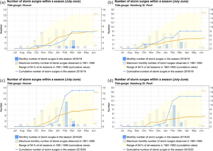
100          X. Liu et al.: Still normal? Near-real-time evaluation of storm surge events in the context of climate change

Figure 1. Locations of the tide gauges used in the monitor. (Credit: Leaflet and maps © OpenStreetMap contributors. Distributed under a
Creative Commons BY-SA License.)

Figure 2. Schematic diagram of the data-processing workflow.

different methods used in practice. The DIN 4049-3 stan-              the water level exceeds the local mean tidal high water level
dard defines a storm surge as an event in which regionally            (MThw, Table 2) by at least 1.5 m. The event is subsequently
defined thresholds are exceeded. These thresholds are de-             further classified as a severe or very severe event when its
fined such that an event with a specific severity can be ex-          maximum water level exceeds MThw by at least 2.5 or 3.5 m.
pected on average once for a given period, e.g., the once-            Because of the different atmospheric and oceanographic con-
in-20-years event (DIN 4049-3, 1994). For their forecasts             ditions, storm surges at the German Baltic Sea coast are di-
and to issue public storm surge warnings, on the other hand,          vided into four classes. Events in which the maximum water
the German Federal Maritime and Hydrographic Agency                   level exceeds the mean water level (MW) by 1.00 m are re-
(Bundesamt für Seeschifffahrt und Hydrographie, BSH) uses             ferred to as storm surge events. Events with water levels of
uniform exceedance thresholds for larger regions (Gönnert,            1.25–1.50 m above MW or 1.50–2.00 m above MW are re-
2003). While each method has advantages and disadvan-                 ferred to as medium or severe events. Cases in which the
tages, the thresholds from the BSH were used in this study, as        maximum water level is higher than 2.00 m above MW are
they are used in public warnings. Accordingly, for the Ger-           referred to as very severe events. While for routine practices,
man North Sea coast, a storm surge event is detected when             mean tidal high water levels and mean water levels are regu-

Nat. Hazards Earth Syst. Sci., 22, 97–116, 2022                                         https://doi.org/10.5194/nhess-22-97-2022
X. Liu et al.: Still normal? Near-real-time evaluation of storm surge events in the context of climate change                           101

Table 1. Summary of the tide gauge records used to calculate the long-term statistics.

      Tide gauge                      Period   Temporal         Data source
                                               resolution
      Husum                     1936–2018      High water       German Federal Waterways and Shipping Administration (WSV), pro-
                                                                vided by the German Federal Institute of Hydrology (BfG)
      Heligoland Binnenhafen    1953–2018      High water       WSV, provided by BfG
      Cuxhaven                  1901–2018      High water       WSV, provided by BfG
                                1919–2018      Hourly           University of Hawaii Sea Level Center (UHSLC) (Caldwell et al., 2015)
      Hamburg St. Pauli         1951–2019      High water       WSV, provided by BfG
      Bremen Weserwehr UW       1954–2019      High water       WSV, provided by BfG
      Norderney                 1901–2018      High water       WSV, provided by BfG and the Coastal Research Station (FSK) of the
                                                                Lower Saxony Water Management, Coastal Defence and Nature Con-
                                                                servation Agency (NLWKN)
      Flensburg                 1955–2019      Hourly           WSV, provided by BfG
      Kiel Holtenau             1955–2019      Hourly           WSV, provided by BfG
      Travemünde                1950–2018      Hourly           WSV, provided by BfG
      Warnemünde                1954–2018      Hourly           WSV, provided by BfG

Table 2. Mean tidal high water levels (MThw) and mean water lev-         June 2019 is referred to as season 2018/2019 and marked as
els (MW) in meters relative to the German reference level NHN            2019 in the plots. The course of a storm surge season and
(Normalhöhennull) of the reference period 1961–1990 for the tide         the monthly distributions are also derived and shown from
gauges along the North Sea and Baltic Sea coasts.                        July to June of the following year. When the ongoing season
                                                                         ends, new long-term statistics are automatically computed, in
              North Sea                        Baltic Sea                which the statistics of the concluded season will be included.
 Tide gauge                  MThw      Gauge                MW
                                                                         2.6   Main features presently implemented
 Husum                       1.58 m    Flensburg        −0.02 m
 Heligoland Binnenhafen      1.07 m    Kiel Holtenau        0m           The monitor was implemented for 10 tide gauges so far. Four
 Cuxhaven                    1.46 m    Travemünde        0.02 m          of them are located at the German North Sea coast; two of
 Hamburg St. Pauli           1.93 m    Warnemünde           0m
                                                                         them are in the Elbe and Weser estuaries; and four of them
 Bremen Weserwehr UW         2.47 m
 Norderney                   1.14 m                                      are along the German Baltic Sea coast (Fig. 1). For each tide
                                                                         gauge, a web page is generated providing figures, texts, and
                                                                         interpretations illustrating (a) the average conditions during
                                                                         the reference period and (b) their long-term trend. Recent
larly updated, we used fixed values calculated over the com-             storm surges are contextualized within the long-term devel-
mon reference period 1961–1990 (Table 2) so that events at               opment, and the ongoing storm surge season is compared to
all gauges can be compared, changes over a longer period                 the reference period. Depending on the availability of his-
can be monitored, and results are presented relative to a fixed          torical data, different measures and statistics are available
reference. In the following, the period 1961–1990 is referred            for each tide gauge. Information on storm surge height and
to as the reference period in the analyses.                              frequency is presented for all gauges, while information on
                                                                         their duration and intensity is provided only for the gauges
2.5    Definition of storm surge seasons
                                                                         where historic hourly data exist (Cuxhaven, Flensburg, Kiel,
At the German North Sea and Baltic Sea coasts, storm surge               Travemünde, and Warnemünde). To illustrate the main fea-
activity is most pronounced in the winter season from Octo-              tures of the monitor, the figures of the season 2019/2020 at
ber to March (Jensen and Müller-Navarra, 2008). In the mon-              the tide gauge Cuxhaven are discussed exemplarily.
itor, the period from July to June of the following year was
therefore used to define and characterize a storm surge sea-
son. Each storm surge season is denoted by the year in which
the season ends. For instance, the period from July 2018 to

https://doi.org/10.5194/nhess-22-97-2022                                             Nat. Hazards Earth Syst. Sci., 22, 97–116, 2022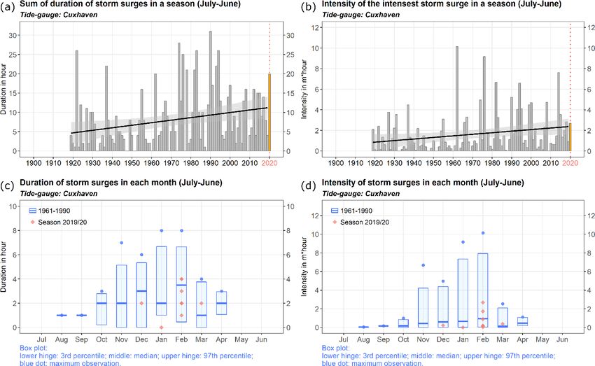
102          X. Liu et al.: Still normal? Near-real-time evaluation of storm surge events in the context of climate change

2.6.1   Storm surge height                                         ment, variability, and change, the number of storm surges per
                                                                   season over time is shown together with its trend (Fig. 4a).
Information on two height indicators is provided, the devel-       Generally, in all plots, a trend that is/is not different from zero
opment of the annual maximum water level over time and the         at the 95 % confidence level is shown by a solid/dashed line.
return period of extremes (Fig. 3). Specifically, the maximum      The severity of the events is marked with different colors to
water level of the current season (red dot) is compared with       illustrate the number of events in the different severity classes
the variations of the annual maxima of the previous seasons        in each season. Again the current season is highlighted in
(black curve) (Fig. 3a). The plot allows for a quick visual-       red. While still ongoing, it can already and preliminarily be
ization of the observed long-term changes and the extent to        put into context with previous seasons, long-term variability,
which the highest water level in the ongoing season is un-         and change.
usual. For an easy visualization, the current season is high-         The second plot (Fig. 4b) was designed to illustrate the
lighted in all the annual plots by a vertical red-dotted line.     course of the ongoing season. It can be used to assess, for
The gray line provides an estimate of the linear trend with        example, if the onset of a storm surge season was very early
the gray-shaded area representing the 95 % confidence in-          or late, if there was an unusual number of events within a
terval. The trend line is shown in solid when the estimated        particular month, or if the whole season is unusually active
trend is significantly different from zero at the level of 95 %    or inactive compared to the average annual cycle. For this,
and dashed otherwise. The scale on the left axis is labeled as     the number of events in each month of the current season
the water level relative to the German reference level (Nor-       (blue bars) can be compared with the maximum number of
malhöhennull, NHN), while the right axis is labeled about          events in the corresponding month over the reference period
the severity classification of storm surges (water level rela-     (1961–1990, gray bars). Further, the blue curve shows the
tive to MThw for the North Sea coast or relative to MW for         cumulative number of events from the beginning of the cur-
the Baltic Sea coast).                                             rent season until the day of the website visit. It can be com-
   The second plot provides estimates of the return periods        pared to the reference given by the 50th percentile (orange
of the storm surges that have occurred in the current ongoing      curve) and the range between the 3rd and the 97th percentiles
season (Fig. 3b). Return periods are widely used to estimate       (yellow-shaded area) of the reference period. For example,
the likelihood and severity of extreme events (e.g., Haigh et      when the blue curve remains below the orange one, this indi-
al., 2015; Wahl et al., 2017). To estimate the return period of    cates that fewer events than usual were observed so far. If the
storm surges, we fitted a generalized extreme value (GEV)          blue curve is above the orange line but still within the yellow-
distribution to the annual maximum values (Hennemuth et            shaded area, this suggests that the frequency of such a season
al., 2013). Here annual maxima refer to the block maxima           is still within a normal range but already belongs to the more
within the historic storm surge seasons. The parameters of         active ones. If the blue curve exceeds the yellow-shaded area,
the distribution (location, scale, and shape) were derived by      indications for an exceptionally active season do exist.
using the maximum-likelihood estimation (MLE).
   Figure 3b displays the extreme value distribution (dark-        2.6.3   Storm surge duration and intensity
gray curve) estimated from the historical data for Cuxhaven
together with its 95 % confidence interval (two light-gray         In addition to storm surge height and frequency, duration and
lines). This fit is subsequently used to evaluate the return pe-   intensity are widely used measures to describe the charac-
riod of the latest (ongoing) storm surges in near real time.       teristics of storm surges (Cid et al., 2016; Zhang et al., 2000)
When an event occurs, a colored symbol whose color de-             that are also important from the perspective of coastal protec-
notes its severity (green – minor; blue – severe; red – very       tion and risk management (e.g., Kodeih et al., 2019). There-
severe) is added. Additionally, an entry on the top of the list    fore, information on both measures was included in the mon-
of current events is generated (right). In the example season      itor, although it can only be provided for those tide gauges
(Fig. 3b), several smaller events with return periods of less      where long-term hourly data were available. In the following
than 5 years and a larger event with a return period between       analyses, duration denotes the number of hours for which the
about 5–10 years can be identified. To further put the recent      water level exceeds the given storm surge threshold, while
events into perspective, a list of the five severest historical    intensity refers to the area between the water level measure-
events during the available period (seasons 1901–2019 here)        ments and the storm surge threshold and has units of me-
is given below the list of events of the current season. These     ter × hour (m h). Regarding storm surge duration, the sea-
are represented by gray open circles with different sizes in-      sonal sum is a key indicator for coastal erosion. Regarding
dicating their magnitudes.                                         intensity, the maximum intensity of storm surges in a season
                                                                   is also critical for potential damages to coastal infrastructure.
2.6.2   Storm surge frequency                                         In the monitor, the total duration and the maximum inten-
                                                                   sity of storm surges in each season are both shown within a
Similarly, two plots assessing the frequency of storm surges       long-term context (Fig. 5). In both cases, the current season
are generated (Fig. 4). To visualize the long-term develop-        is highlighted with an orange bar to be easily separable from

Nat. Hazards Earth Syst. Sci., 22, 97–116, 2022                                       https://doi.org/10.5194/nhess-22-97-2022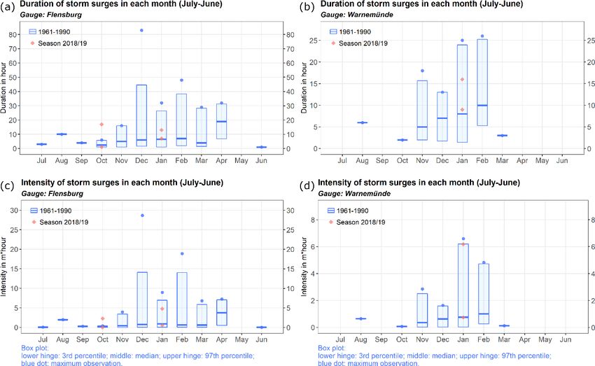
X. Liu et al.: Still normal? Near-real-time evaluation of storm surge events in the context of climate change                                 103

Figure 3. (a) Maximum water level per storm surge season (past seasons – black; ongoing season – red) in meters (left ordinate: relative
to NHN; right ordinate: relative to MThw of the reference period) and corresponding linear trend at Cuxhaven (gray line) together with
the 95 % confidence interval (light-gray band). (b) Return periods of storm surge events at Cuxhaven from the past (gray symbols) and the
ongoing season (colored symbols; green – minor; blue – severe; red – very severe events) together with the estimated distribution (dark-gray
curve) and the corresponding 95 % confidence band (area between the light-gray curves) derived from past annual maxima. The events of the
ongoing season and the top five severe historical events in the available period are listed on the right. Please note that the date formats in this
figure are month-day and year-month-day.

Figure 4. (a) Number of storm surges per season (colored bars; green – minor; blue – severe; red – very severe) and the corresponding
linear trend (gray line) together with the 95 % confidence band (gray shaded) at Cuxhaven. (b) Development of the ongoing storm surge
season illustrated by the number of storm surges per month (blue) and their sum since the onset of the season (blue line) at Cuxhaven. For
contextualization, also the historical monthly maximum number of events (gray bars) and the 50th percentile (orange curve) and the range
between the 3rd and 97th percentiles (yellow-shaded area) from the cumulative number of events in the reference period 1961–1990 are
shown.

the previous seasons (gray bars). Assessment of single events               dots, which indicate whether an event lasted longer or was
within a season can be derived from Fig. 5c and d, in which                 more intense in comparison to the monthly statistics of the
the events of the current seasons (red dots) are shown relative             reference period.
to the monthly distributions derived from historical data. The
historical reference (blue) is illustrated in the form of a box
plot bounded by the 3rd and 97th percentiles. The median                    3   Long-term changes
is given by the solid horizontal blue line, and the historical
                                                                            In this section, the capabilities of the monitor in supporting
maximum in each month is denoted by the blue dot. Assess-
                                                                            assessments of long-term changes are briefly illustrated.
ment can be obtained from the relative positions of the red

https://doi.org/10.5194/nhess-22-97-2022                                                Nat. Hazards Earth Syst. Sci., 22, 97–116, 2022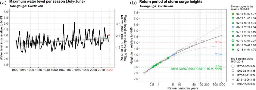
104           X. Liu et al.: Still normal? Near-real-time evaluation of storm surge events in the context of climate change

Figure 5. (a, b) Total duration and maximum intensity of storm surges per season at Cuxhaven for past (gray bars) and the ongoing (orange
bar) seasons together with the linear trend (black line) and the 95 % confidence interval. (c, d) Box plots for the monthly duration and
intensity of storm surges in the reference period (blue box – 3rd to 97th percentile; blue line – median; blue point – maximum) together with
the events of the ongoing season (orange).

3.1     North Sea coast                                                  the highest since the beginning of data availability. Among
                                                                         the analyzed North Sea tide gauges, the highest water level
3.1.1    Height                                                          since the 1950s occurred on 3 January 1976 at Hamburg St.
                                                                         Pauli with about 4.5 m above MThw. In the last decade, a
The annual maximum water level increased at all tide gauges              storm surge in December 2013 represents the highest event.
over the available periods (e.g., Figs. 3a, 6). Except for He-           At some gauges (Cuxhaven, Hamburg, Bremen, and Norder-
ligoland, the trends are significantly different from zero at            ney), it is among the five highest events over the available
the 95 % confidence level. The mean increase of the annual               periods.
maximum water level since 1950 is about 20–40 cm at the
coastal gauges and about 60–100 cm at the estuarine gauges               3.1.2   Frequency
Bremen and Hamburg. The reasons for the increases are still
discussed in the literature but are likely to be the result of the       Annual storm surge frequency increased at all gauges
interplay between several factors, such as mean sea level rise,          (e.g., Figs. 4a, 7). Except for Heligoland, the trends are sig-
variability in the wind climate, astronomical tide cycles, and           nificantly different from zero at the 95 % confidence level. In
the implementation of hydro-engineering measures with dif-               the 1950s, about one to three storm surges usually occurred
ferent contributions at the coast and in the estuaries (e.g., von        in a season. Over the past few decades, the annual number of
Storch and Woth, 2008; von Storch et al., 2008; Hein et al.,             storm surges has increased by about one at Heligoland and
2021; Jensen et al., 2021).                                              Norderney, and it has nearly doubled at Husum and Cux-
   Although the trends are positive, the annual maximum wa-              haven. At the estuarine gauges, storm surge frequency has
ter level strongly varies between seasons and from gauge to              increased even more strongly. On average, there are about
gauge. Among the gauges, either the storm surge of Febru-                5 times as many storm surges per season nowadays as there
ary 1962 (Heligoland, Bremen, and Norderney) or the storm                were in the 1950s. In addition to the positive trends, the num-
surge of January 1976 (Husum, Cuxhaven, and Hamburg) is                  ber of events also varies from season to season and from

Nat. Hazards Earth Syst. Sci., 22, 97–116, 2022                                             https://doi.org/10.5194/nhess-22-97-2022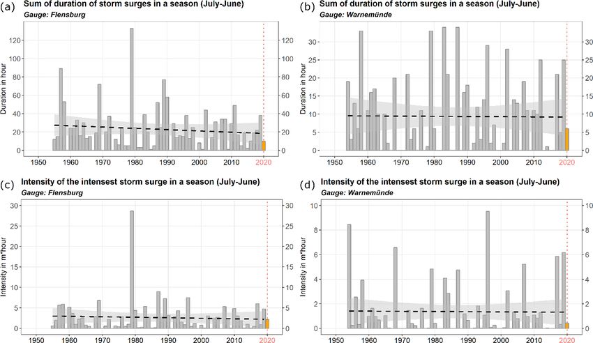
X. Liu et al.: Still normal? Near-real-time evaluation of storm surge events in the context of climate change                      105

Figure 6. As Fig. 3a but for the tide gauges Husum (a) and Hamburg St. Pauli (b).

gauge to gauge. In general, there are fewer events at He-              (e.g., Meinke, 1999). Although no significant changes in the
ligoland, Cuxhaven, and Norderney, while events occur more             extremes could be detected, the mean sea level has increased
frequently at Husum, Hamburg, and Bremen. This may be                  along the German Baltic Sea coast (e.g., Weisse and Meinke,
not only due to differences in the specific configuration of           2016; Weisse et al., 2021) and is expected to rise further
the coastline and bathymetry relative to the prevailing wind           in the future (e.g., Grinsted, 2015; Hieronymus and Kalén,
direction during storm surges that make a location more or             2020). Therefore, it is likely that the annual maximum wa-
less susceptible to storm surges (e.g., Gönnert, 2003) but             ter levels may increase in the future as well. Thus, ongoing
also partly an effect of the common threshold used to detect           monitoring is important, although no significant trends in the
surges in the monitor (see Sect. 2).                                   annual maxima water level could be detected so far.
                                                                          Over the past 7 decades, the annual maximum water level
3.1.3    Duration and intensity                                        has varied between about 0.7 and 2.0 m above MW at the an-
                                                                       alyzed gauges. The average maximum water level is around
Due to the limited availability of high-temporal-resolution            1.2 m above MW. The data in the monitor do not include
data, the statistics for storm surge duration and intensity can        the highest storm surge at the German Baltic Sea coast
only be evaluated for Cuxhaven. As introduced in Sect. 2.6.3,          that occurred on 13 November 1872 (Jensen and Müller-
the total duration of all events in a season and the intensity         Navarra, 2008; Rosenhagen and Bork, 2009; von Storch et
of the most intense event in a season are evaluated (Fig. 5a,          al., 2015; Weisse and Meinke, 2016) and for which only
b). For both measures, upward trends significantly different           limited reliable measurements are available. According to
from zero could be inferred. Specifically, both measures have          these, the maximum water level was about 3.3 m above MW
about doubled since the 1920s. The annual total duration in-           (e.g., Jensen and Müller-Navarra, 2008) along the southwest-
creased from about 5 to 12 h, and the annual maximum inten-            ern coast of the Baltic Sea. This is much higher than any ex-
sity increased from about 1 m h to about 3 m h. This is likely         treme event that occurred later in this region. Since the 1950s,
caused by an increase in mean sea level that raised the base-          none of the water levels at the analyzed Baltic Sea gauges
line upon which wind-induced fluctuations act rather than a            exceeded 2 m above MW (Fig. 8). However, this value was
change in storm climate (e.g., Weisse et al., 2012; Weisse and         nearly hit in Travemünde on 4 January 1954 when the water
Meinke, 2016). Averaged over the reference period, the mean            level reached a value of 1.97 m above MW and in Kiel on
values of the total duration and the maximum intensity were            4 November 1995 when the water level reached a maximum
about 10 h and 2 m h, respectively.                                    of 1.96 m above MW (not shown).

3.2     Baltic Sea coast                                               3.2.2   Frequency

3.2.1    Height                                                        The storm surge frequency at the analyzed Baltic Sea gauges
                                                                       shows pronounced interannual and decadal variability. Over
At the German Baltic Sea coast, the annual maximum water               the available periods since the 1950s, the frequency has var-
levels show strong variability over the available period. Lin-         ied between zero and nine events. Except for Warnemünde,
ear trends within this period vary in their signs from gauge           all gauges show a maximum of events observed in the sea-
to gauge and because of the strong interannual variability;            son 1989/1990 (e.g., Flensburg, Fig. 9a). In Warnemünde the
none of the trends is significantly different from zero at the         highest number of events in a season was five and was ob-
95 % confidence level (Fig. 8). This is consistent with the            served in 2001/2002 (Fig. 9b). Trends in storm surge fre-
results based on annual data, which cover a longer period              quency are not significant at all gauges (e.g., Fig. 9). As

https://doi.org/10.5194/nhess-22-97-2022                                            Nat. Hazards Earth Syst. Sci., 22, 97–116, 2022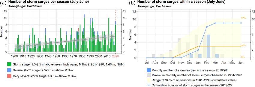
106 X. Liu et al.: Still normal? Near-real-time evaluation of storm surge events in the context of climate change
Figure 7. As Fig. 4a but for the tide gauges Husum (a) and Hamburg St. Pauli (b).
Figure 8. As Fig. 3a but for the gauges Flensburg (a) and Warnemünde (b).
mean sea level increased over the period (e.g., Weisse et al., total duration and the maximum intensity of storm surges per
2021), insignificant trends in the extremes may be due to the season show strong variabilities. Trends at all gauges vary
large interannual variability in the extremes that hamper de- around zero and are not statistically different from zero at
tection in relatively short records. Overall, the storm climate the 95 % confidence level (Fig. 10). This is consistent with
over the area does not show significant trends (e.g., Weisse et the findings from other studies that analyzed data from model
al., 2021). This result is consistent with other studies analyz- hindcasts over different periods (e.g., Weidemann, 2014).
ing different periods (e.g., 1883–1997 in Meinke, 1999, and
1948–2011 in Weidemann, 2014) and in which the effects of
mean sea level rise have been excluded. Moreover, the wind 4 Evaluation of recent storm surge seasons
climate over the Baltic Sea shows large interdecadal variabil-
ity: for the last 6 decades, an increase in the number of days In this section, cases from two recent storm surge seasons
with westerly components has been detected during winter (2018/2019 and 2019/2020) are exemplarily discussed to il-
(Gräwe et al., 2019; Lehmann et al., 2011), while days with lustrate the capabilities of the monitor in aiding the identi-
easterly winds have decreased (Gräwe et al., 2019). Since fication of unusual events and/or seasons together with re-
storm surges in the southwestern Baltic Sea are mainly con- gional differences.
nected with strong easterly winds, this variability in wind cli-
mate could further contribute to the insignificant trends in 4.1 North Sea coast
storm surge activity since 1950, against the background of
rising mean sea level. 4.1.1 Height
3.2.3 Duration and intensity In the season 2018/2019, the annual maximum water levels
at all gauges fell into the lowest category of severity (1.5–
Information on duration and intensity can be derived at all se- 2.5 m above MThw) (e.g., Figs. 3a, 6). This immediately im-
lected Baltic Sea gauges, since hourly data are available. The plies that all events observed in the season were minor (green
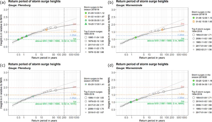
Nat. Hazards Earth Syst. Sci., 22, 97–116, 2022 https://doi.org/10.5194/nhess-22-97-2022X. Liu et al.: Still normal? Near-real-time evaluation of storm surge events in the context of climate change 107 Figure 9. As Fig. 4a but for the gauges Flensburg (a) and Warnemünde (b). Figure 10. (a, b) As Fig. 5a but for the gauges Flensburg (a) and Warnemünde (b). (c, d) As Fig. 5b but for the gauges Flensburg (c) and Warnemünde (d). marks in Fig. 11a, b). Except for Husum, the highest event in cur several times a year, and the season 2018/2019 was not the season occurred on 8 January 2019, and its return pe- unusual in terms of storm surge height. riod varies between about 1 and 3 years depending on the Compared to the season 2018/2019, higher annual max- tide gauge. For Heligoland and Norderney, this was also the imum water levels were observed in the following sea- only event detected in this season using the thresholds de- son, 2019/2020 (Figs. 3a, 6). During 10–12 February 2020, fined in Sect. 2. It should be noted that the use of different a storm named Sabine by the German Weather Service thresholds (e.g., DIN 4049-3, 1994) can lead to different re- (Deutscher Wetterdienst) (Haeseler et al., 2020) and Ciara sults. At other gauges, more events were registered, but they and Elsa by the UK Met Office and Norwegian Meteorolog- only slightly exceeded the lowest threshold (e.g., Husum and ical Institute, respectively, induced a series of consecutive Hamburg in Fig. 11a, b). On average, such events may oc- storm surges. The highest water levels of the season were https://doi.org/10.5194/nhess-22-97-2022 Nat. Hazards Earth Syst. Sci., 22, 97–116, 2022
108          X. Liu et al.: Still normal? Near-real-time evaluation of storm surge events in the context of climate change

Figure 11. As Fig. 3b but for the tide gauges Husum (a, c) and Hamburg St. Pauli (b, d): (a, b) season 2018/2019 and (c, d) season 2019/2020.
Please note that the date formats in this figure are month-day and year-month-day.

observed during these days. The estimated return period of               Husum (Fig. 12a), and eight events were observed at Ham-
the highest event varies from 3 to 8 years at different gauges           burg (Fig. 12b) and Bremen (not shown).
(Fig. 11c, d). In addition to this series of events, more minor             In the season 2019/2020, the number of events was at least
events were detected at Husum, Cuxhaven, Hamburg, and                    twice as high at five of the six tide gauges. Especially, the
Bremen. They are categorized as minor events with estimated              number of 13 events at Husum is remarkable and exceeds
return periods shorter than 1 year, indicating that such minor           the 3rd–97th percentile of the reference period (Fig. 12c).
events are common for these gauges. While somewhat more                  The season ranks among the top three in terms of storm surge
active than the previous season, again the season 2019/2020              frequencies at this gauge (Fig. 7a).
was not unusual in terms of storm surge height.                             A look at the course of the season and the long-term
                                                                         average reveal that the first storm surges usually occur in
4.1.2   Frequency                                                        November or December and that the majority occur between
                                                                         November and February (Fig. 12). The course of the sea-
In terms of storm surge frequency, the two seasons                       son 2018/2019 broadly followed this development along the
2018/2019 and 2019/2020 differ significantly. In the sea-                long-term median (Fig. 12a, b). For some gauges, frequen-
son 2018/2019, storm surge frequency is around the aver-                 cies eventually exceeded the long-term median, but the val-
age frequency of the reference period. A total of one or two             ues remained well below the 97th percentiles. Moreover, the
events was observed at Cuxhaven (Fig. 4a), Heligoland, and               numbers of events in the individual months were exceptional
Norderney (not shown), whereas six events were observed at               nowhere.

Nat. Hazards Earth Syst. Sci., 22, 97–116, 2022                                             https://doi.org/10.5194/nhess-22-97-2022
X. Liu et al.: Still normal? Near-real-time evaluation of storm surge events in the context of climate change 109
Figure 12. As Fig. 4b but for the tide gauges Husum (a, c) and Hamburg St. Pauli (b, d): (a, b) season 2018/2019 and (c, d) season 2019/2020.
In contrast, the season 2019/2020 was substantially differ- discussion above), while the individual events were neither
ent. The season initially started late, and the storm surge fre- exceptionally intense nor long-lasting (Fig. 5c, d).
quencies were moderate and mostly below the long-term me- In summary, for the German North Sea coast, the storm
dian. This character substantially changed in February when season 2018/2019 represents a rather typical storm surge sea-
the storm Sabine caused a large number of events within a son in all aspects. All detected events were relatively low,
relatively short period (Fig. 12c, d). For example at Husum, and their return periods were mostly shorter than 1 year. Al-
nine events (five of which were caused within only about 2 d) though the number of events at some gauges was slightly
were registered in February 2020, which exceeds the maxi- above the average level, it is still far from the upper bound
mum of seven events detected so far in February (Fig. 9c). defined by the long-term 97th percentile. In contrast, the sea-
Consequently, the cumulated number of events in the season son 2019/2020 was more active and unusual in some aspects.
exceeds the 3rd–97th percentile range, and the season even- It was characterized by a slow onset, which was more than
tually represented a rather unusual season in terms of storm compensated by an unusual series of events in February. In
surge frequency, although their height was mostly moderate. consequence, the total number of events at the end of the sea-
son was only slightly below or even above the upper bound
4.1.3 Duration and intensity of the long-term distribution. While the surges were mostly
moderate in height, the total duration of the storm surges was
The two storm surge seasons also differ in terms of their total also doubled compared to the reference period.
duration and their maximum intensity. This is demonstrated
exemplarily for Cuxhaven (Fig. 5). Here, both measures were
significantly higher in the season 2019/2020, especially the
total duration. In this case, this can be attributed to the un-
usually large number of shorter events in this season (see
https://doi.org/10.5194/nhess-22-97-2022 Nat. Hazards Earth Syst. Sci., 22, 97–116, 2022110 X. Liu et al.: Still normal? Near-real-time evaluation of storm surge events in the context of climate change
Figure 13. As Fig. 3b but for the gauges Flensburg (a, c) and Warnemünde (b, d): (a, b) season 2018/2019 and (c, d) season 2019/2020.
Please note that the date formats in this figure are month-day and year-month-day.
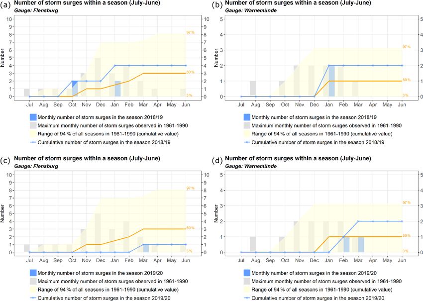
4.2 Baltic Sea coast 4.2.2 Frequency
4.2.1 Height
In contrast to the North Sea, both seasons in the Baltic
Contrary to the North Sea where the two storm surge seasons Sea were relatively typical in terms of storm surge fre-
2018/2019 and 2019/2020 were rather similar in height but quency. This is again shown exemplarily for Travemünde and
differed in frequencies, both seasons differed in height in the Warnemünde (Fig. 14). While in 2018/2019 the storm surge
Baltic Sea with the first season being the stronger one. This frequency at both gauges was slightly above the average of
illustrates that in both areas different meteorological condi- the reference period, in 2019/2020 it was below average in
tions are required to generate storm surges. The differences Flensburg and above average in Warnemünde. In all cases,
between both seasons are shown exemplarily for Flensburg values fell within usual ranges, except for the maximum
and Warnemünde (Fig. 13). At both gauges, the highest storm number of surges observed in October 2018 in Flensburg.
surge in the season 2018/2019 occurred on 2 January 2019 Note, however, that total numbers are small, which makes
and was caused by the storm Zeetje (Perlet, 2019). The max- comparisons less robust.
imum water levels reached 1.67 and 1.65 m, respectively, at
Flensburg and Warnemünde. In both cases, the event repre- 4.2.3 Duration and intensity
sented severe storm surges. In Warnemünde its height was
very close to the highest value of 1.71 m in the record, and the
estimated return period of the event in January 2019 was be- Contrary to the North Sea, the season 2018/2019 was more
tween about 50–60 years. At the other gauges, the frequency active than 2019/2020 in terms of total duration and intensity
of such events is somewhat larger, and the return periods of (Fig. 10). While for the North Sea, the season 2019/2020 was
the January 2019 event vary between about 10–20 years. Re- outstanding in terms of duration due to a series of moderate
garding height, the season 2019/2020 was less active with events, for the Baltic Sea the season 2018/2019 stands out in
events having return periods well below 5 years (Fig. 13). terms of intensity caused by a major event in January 2019
(Fig. 15). In Flensburg also the duration and intensity of the
event on 29 October 2018 were exceptionally high (Fig. 15a,
c). Again this illustrates that different atmospheric conditions
Nat. Hazards Earth Syst. Sci., 22, 97–116, 2022 https://doi.org/10.5194/nhess-22-97-2022X. Liu et al.: Still normal? Near-real-time evaluation of storm surge events in the context of climate change 111
Figure 14. As Fig. 4b but for the gauges Flensburg (a, c) and Warnemünde (b, d): (a, b) season 2018/2019 and (c, d) season 2019/2020.
are required to trigger storm surges along the German North ation of extremes, for example, to assess in near real time if
Sea and Baltic Sea coasts. and to what extent an event or a season is unusual compared
to the statistics of the extreme events in the past decades.
Measures to assess long-term changes can also be inferred
5 Discussion and summary from the monitor. Because of the existing risk and the ex-
pected future developments, such information can be highly
A new tool and approach for monitoring the storm surge haz- relevant for decision making (e.g., Kodeih, 2018; Kodeih et
ard in the context of long-term variability and climate change al., 2019; Weisse et al., 2015) or within public debate.
were proposed. They aim at providing near-real-time infor- The monitor also documents long-term changes in storm
mation for the evaluation and contextualization of ongoing surge climate. Such changes can in principle originate from
extremes and at bridging the gap between the availability of various factors, such as changes in storm activity, astronom-
real-time data and the considerable time delay before assess- ical tide cycles, or sea level rise. Locally, waterworks may
ments are published. The approach was implemented into also play a role. To date, there is no clear evidence suggest-
a prototype web tool (the storm surge monitor) and imple- ing a significant long-term change of storm activity in the
mented exemplarily for the German North Sea and Baltic German coastal regions (Feser et al., 2015; Krieger et al.,
Sea coasts. With the help of the monitor, storm surges are de- 2020; Krueger et al., 2019; Stendel et al., 2016; Weisse et
tected in real time and are set into a climatological context in al., 2012). For the North Sea gauges, likely, the observed
near real time. This way, not only an assessment of the cur- changes in storm surge climate are largely related to the local
rent storm surge season or ongoing events is achieved, but mean sea level rise (e.g., Weisse et al., 2012; Woodworth et
also the development over the past seasons is documented. al., 2011). Rising relative sea levels in the area, for the most
The tool aims at providing easily accessible information to part, not only are related to global mean sea level rise and cli-
the public, scientists, and stakeholders that aid in the evalu-
https://doi.org/10.5194/nhess-22-97-2022 Nat. Hazards Earth Syst. Sci., 22, 97–116, 2022112 X. Liu et al.: Still normal? Near-real-time evaluation of storm surge events in the context of climate change Figure 15. (a, b) As Fig. 5c but for the gauges Flensburg (a) and Warnemünde (b). (c, d) As Fig. 5d but for the gauges Flensburg (c) and Warnemünde (d). mate change but also contain contributions from non-climatic ous such efforts do exist. These tools provide online ac- factors such as land subsidence. The latter may result from cess to the statistics of extreme water levels or document natural phenomena (e.g., GIA) or local anthropogenic activ- the severity and consequences of historical flooding. Ex- ities (e.g., groundwater extraction, dredging, or waterworks) amples are the Extreme Water Levels site from NOAA (e.g., Rovere et al., 2016; Stammer et al., 2013; Tamisiea and (https://tidesandcurrents.noaa.gov/est/, last access: 14 Jan- Mitrovica, 2011). uary 2022) or the SurgeWatch site for the UK coast (https: At the analyzed gauges at the German Baltic Sea coast, no //www.surgewatch.org/, last access: 14 January 2022, Haigh significant long-term change in storm surge activity has been et al., 2015). We built upon experiences from developing detected so far. For the annual maximum water levels, this such tools, but contrary to existing ones our storm surge mon- is in agreement with, e.g., the results of Meinke (1999) and itor focuses on the near-real-time evaluation and contextual- the review in Weisse et al. (2021). Similarly, non-significant ization of extremes against the background of long-term vari- trends have been found for storm surge frequency, also in ability and change to provide an up-to-date and continuously agreement with previous studies (e.g., Weidemann, 2014). available piece for coastal climate services. Both the mon- It is plausible that storm surge height, frequency, duration, itor and the statistics are freely available online. They are and intensity may change in the future, as sea level contin- expected to be useful and meaningful to the public. In partic- ues to rise along the German North Sea and Baltic Sea coasts ular, the monitor was found to be useful to the media, since (e.g., Grinsted, 2015; Weisse and Meinke, 2016; Hieronymus it fits their needs to focus on actual threats and to contextual- and Kalén, 2020; Weisse et al., 2021). Thus, continuous mon- ize them within a scientific frame. After the implementation itoring of the storm surge climate in a climatological context of the monitor, numerous interview requests were served and may foster early detection and attribution and support adap- background information was provided based on the monitor. tation and public debate. The monitor is further relevant to multi-sector coastal Nowadays, web-based applications are frequently used stakeholders who demand such information for coastal flood tools to develop links between the results of scientific re- risk management and planning. For example, presently a dis- search and public demands. For sea level extremes, vari- cussion is ongoing with users asking for an extension in- Nat. Hazards Earth Syst. Sci., 22, 97–116, 2022 https://doi.org/10.5194/nhess-22-97-2022
X. Liu et al.: Still normal? Near-real-time evaluation of storm surge events in the context of climate change                          113

cluding also thresholds following the definitions given in the          (European Research Area for Climate Services) framework (EU
DIN 4049-3 standard (DIN4049-3, 1994). Further and in-                  grant agreement no. 690462).
terestingly, the series of storm surges that made the season
2019/2020 outstanding along the North Sea coast occurred                The article processing charges for this open-access
shortly after the conclusion of the transdisciplinary project           publication were covered by the Helmholtz-Zentrum Hereon.
EXTREMENESS (Weisse et al., 2019) in which physically
plausible but yet unobserved extremes and their potential im-
                                                                        Review statement. This paper was edited by Paolo Tarolli and re-
pacts were discussed and modeled. One type of such po-
                                                                        viewed by Klaus Grosfeld and Andreas Sterl.
tentially high-impact events identified by stakeholders was
a series of storm surges that, even when only of moder-
ate heights, may provide challenges for coastal protection
(Schaper et al., 2019; Weisse et al., 2019).                            References
   The monitor can further serve for educational purposes,
for example, illustrating changing storm surge activity at              Arns, A., Dangendorf, S., Jensen, J., Talke, S., Bender, J.,
German coasts. Finally, it can also be useful to researchers              and Pattiaratchi, C.: Sea-level rise induced amplification
                                                                          of coastal protection design heights, Sci Rep., 7, 40171,
as auxiliary information supporting their research. We argue
                                                                          https://doi.org/10.1038/srep40171, 2017.
that the tool has the potential to be developed into a larger           Barbosa, S. M.: Quantile trends in Baltic sea level, Geophys. Res.
suite of tools including, for example, other regions or other             Lett., 35, L22704, https://doi.org/10.1029/2008gl035182, 2008.
coastal hazards such as sea level rise or storm activity.               Butler, A., Heffernan, J. E., Tawn, J. A., and Flather, R. A.: Trend
                                                                          estimation in extremes of synthetic North Sea surges, J. Roy.
                                                                          Stat. Soc. C.-App., 56, 395–414, https://doi.org/10.1111/j.1467-
Code availability. The code used for data pre- and post-processing        9876.2007.00583.x, 2007.
is available on request from the authors.                               Caldwell, P. C., Merrifield, M. A., and Thompson, P. R.: Sea level
                                                                          measured by tide gauges from global oceans – the Joint Archive
                                                                          for Sea Level holdings (NCEI Accession 0019568), Version 5.5,
Data availability. The data used in this paper are available from         NOAA National Centers for Environmental Information [data
the third party sources listed in Table 1. Real-time data are             set], https://doi.org/10.7289/V5V40S7W, 2015.
available from https://www.pegelonline.wsv.de/ (PEGELONLINE,            Cid, A., Menendez, M., Castanedo, S., Abascal, A. J., Mendez, F.
2022) as described in the text. Near-real-time analyzes are available     J., and Medina, R.: Long-term changes in the frequency, intensity
from the monitor websites in German (https://sturmflut-monitor.           and duration of extreme storm surge events in southern Europe,
de, STURMFLUT-MONITOR, 2022) and in English (https://                     Clim. Dynam., 46, 1503–1516, https://doi.org/10.1007/s00382-
stormsurge-monitor.eu, STORMSURGE-MONITOR, 2022).                         015-2659-1, 2016.
                                                                        Dangendorf, S., Müller-Navarra, S., Jensen, J., Schenk, F., Wahl,
                                                                          T., and Weisse, R.: North Sea storminess from a novel storm
Author contributions. RW and IM initiated the idea of the storm           surge record since AD 1843, J. Climate, 27, 3582–3595,
monitor and designed it. XL processed the data, performed the anal-       https://doi.org/10.1175/jcli-d-13-00427.1, 2014.
yses, and programmed the web tool. All authors equally contributed      Deutschländer, T., Friedrich, K., Haeseler, S., and Lefebvre, C.:
to the preparation of the manuscript. The revised version including       Severe storm XAVER across northern Europe from 5 to 7
the suggestions from the reviewers was prepared by RW and IM.             December 2013, Deutscher Wetterdienst, available at: https:
                                                                          //www.dwd.de/EN/ourservices/specialevents/storms/20131230_
                                                                          XAVER_europe_en.pdf?__blob=publicationFile&v=20131234
                                                                          (last access: 14 January 2022), 2013.
Competing interests. The contact author has declared that neither
                                                                        DIN 4049-3: Hydrologie. Teil 3: Begriffe zur quantitativen Hy-
they nor their co-authors have any competing interests.
                                                                          drologie 135DVWK (Deutscher Verband für Wasserwirtschaft
                                                                          und Kulturbau) (1999): Statistische Analyse von Hochwasser-
                                                                          abflüssen, DVWK 215/1999, Verlag Paul Parey, Hamburg,
Disclaimer. Publisher’s note: Copernicus Publications remains             https://doi.org/10.31030/2644617, 1994.
neutral with regard to jurisdictional claims in published maps and      Feser, F., Barcikowska, M., Krueger, O., Schenk, F., Weisse, R.,
institutional affiliations.                                               and Xia, L.: Storminess over the North Atlantic and northwest-
                                                                          ern Europe – A review, Q. J. Roy. Meteor. Soc., 141, 350–382,
                                                                          https://doi.org/10.1002/qj.2364, 2015.
Acknowledgements. The map in Fig. 1 is generated by Leaflet and         Feuchter, D., Jörg, C., Rosenhagen, G., Auchmann, R., Martius,
© OpenStreetMap contributors.                                             O., and Brönnimann, S.: The 1872 Baltic Sea storm surge,
                                                                          in: Weather extremes during the past 140 years, edited by:
                                                                          Brönnimann, S. and Martius, O., Geographica Bernensia G89,
Financial support. This work was financially supported by the Eu-         https://doi.org/10.4480/GB2013.G89.10, 2013.
ropean Union through the project “European advances on CLImate          Gaslikova, L., Grabemann, I., and Groll, N.: Changes in
Services for Coasts and SEAs” (ECLISEA) under the ERA4CS                  North Sea storm surge conditions for four transient fu-

https://doi.org/10.5194/nhess-22-97-2022                                           Nat. Hazards Earth Syst. Sci., 22, 97–116, 2022
You can also read