Study of Electronic Speed Control Strategies for a Fixed Battery, Motor and Propeller Aircraft Propulsion Set
←
→
Page content transcription
If your browser does not render page correctly, please read the page content below

Study of Electronic Speed Control Strategies for
  a Fixed Battery, Motor and Propeller Aircraft
                                Propulsion Set
                                      (versão final após defesa)

                                                  Viktor Zombori

                       Dissertação para obtenção do Grau de Mestre em
                                      Engenharia Aeronáutica
                                            (Ciclo de estudos integrado)

             Orientador: Prof. Doutor Miguel Ângelo Rodrigues Silvestre

                                        Covilhã, dezembro de 2021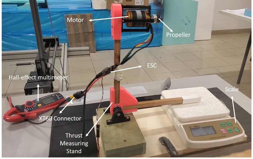
ii
Acknowledgements

I would like to express my gratitude to my supervisor, Professor Miguel Silvestre, for all the
guidance provided throughout the realization of this thesis.

I would also like to thank Jorge Rebelo and Pedro Alves for sharing their time and knowledge,
which were crucial to make the present work happen.

A special thank you to my family for their love and support in every way.

A big thank you to my friends for all the great moments and for always being there.

                                            iii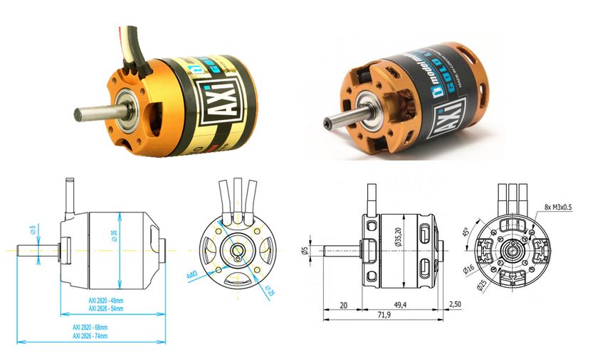
iv
Resumo

No âmbito da participação da equipa AERO@UBI no Air Cargo Challenge 2021/2022, foi
realizado um estudo de um sistema propulsivo elétrico com duas hélices como opção e uma
bateria e motor definidos. Os objetivos passavam por maximizar a tração gerada pelo con-
junto, especialmente a elevadas velocidades de vento relativo, através da adoção da melhor
estratégia de controlo do motor e escolher a melhor das hélices para este propósito. Dois
controladores eletrónicos de velocidade foram selecionados: o Phoenix ICE 75 da Castle Cre-
ations, que realiza comutação trapezoidal, e um A50S da Team Triforce, que opera com field-
oriented control (FOC). Ambos foram testados em condições de tração estática e com vento
relativo, utilizando uma bancada de tração estática e uma instalação experimental montada
em um túnel de vento, respetivamente. Estes testes permitiram perceber qual a influência de
diferentes funcionalidades implementadas nos controladores tais como motor timing e fre-
quência de modelação de comprimento de pulso (PWM rate), bem como várias magnitudes
de field weakening. Os resultados obtidos foram muito positivos: em condições estáticas, o
FOC com field weakening permitiu aumentar a tração estática produzida em mais de 10%
relativamente ao melhor valor obtido com a comutação trapezoidal. Esta diferença foi am-
plificada ainda mais com velocidades crescentes de vento relativo.

Palavras-chave

Motor elétrico, controlo de motor, field-oriented control, field weakening, hélice.

                                            v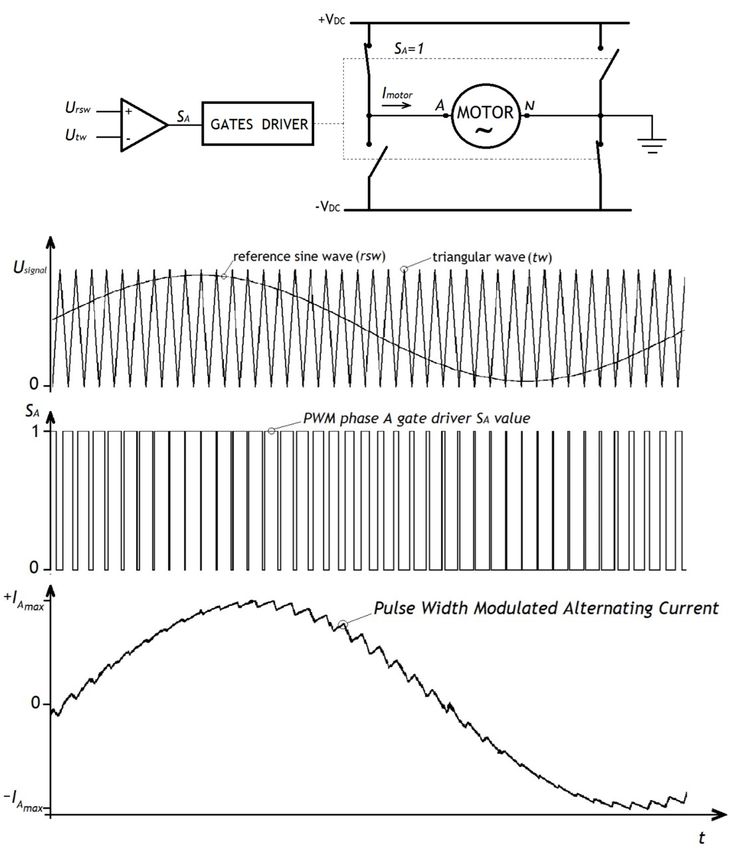
vi

Abstract

A study of an electrical propulsion system with two propeller options and a fixed battery and
motor was performed, in the context of the participation of the AERO@UBI team in the Air
Cargo Challenge 2021/2022. The goals were to maximize the thrust generated by the setup,
specially at high relative wind speed, by means of adopting the best motor control strategy
and to select the better propeller for this purpose. Two electronic speed controllers (ESCs)
were selected: the Castle Creations Phoenix ICE 75, that performs trapezoidal commutation,
and a Team Triforce A50S, which makes use of field-oriented control (FOC). Both were tested
under static condition and with relative wind, using a static thrust stand and an experimental
setup in a wind tunnel, respectively. These tests allowed to understand the influence on the
generated thrust and drawn current of different settings that are implemented on the con-
trollers, such as motor timing and pulse-width modulation (PWM) rate, as well as various
magnitudes of field weakening. The obtained results were very positive: under static condi-
tions, FOC with field weakening allowed to increase the generated static thrust by more than
10% relative to the best value obtained with trapezoidal commutation. This difference was
amplified even more with increasing relative wind speed.

Keywords

Electric motor, motor control, field-oriented control, field weakening, propeller.

                                            vii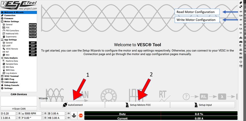
viii
Contents

1   Introduction                                                                                      1
    1.1   Motivation . . . . . . . . . . . . . . . . . . . . . . . . . . . . . . . . . . . . . .      1
    1.2   Scope . . . . . . . . . . . . . . . . . . . . . . . . . . . . . . . . . . . . . . . . .     2
    1.3   Objectives . . . . . . . . . . . . . . . . . . . . . . . . . . . . . . . . . . . . . . .    2
    1.4   Document Structure . . . . . . . . . . . . . . . . . . . . . . . . . . . . . . . . .        2

2 Literature Review                                                                                   5
    2.1   Fundamentals . . . . . . . . . . . . . . . . . . . . . . . . . . . . . . . . . . . .        5
          2.1.1   Brushed DC Motor . . . . . . . . . . . . . . . . . . . . . . . . . . . . . .        5
          2.1.2   Brushless DC Motor . . . . . . . . . . . . . . . . . . . . . . . . . . . . .        6
          2.1.3   Brushless Speed Control . . . . . . . . . . . . . . . . . . . . . . . . . . 10
          2.1.4   BEMF . . . . . . . . . . . . . . . . . . . . . . . . . . . . . . . . . . . . . 10
          2.1.5   Sensored and Sensorless Control . . . . . . . . . . . . . . . . . . . . . .        11
          2.1.6   Motor Control - Trapezoidal, Sinusoidal and FOC . . . . . . . . . . . .            13
          2.1.7   Field Weakening . . . . . . . . . . . . . . . . . . . . . . . . . . . . . . .      16
    2.2 State of the Art . . . . . . . . . . . . . . . . . . . . . . . . . . . . . . . . . . . .     17

3 Methodology                                                                                        19
    3.1   Motor . . . . . . . . . . . . . . . . . . . . . . . . . . . . . . . . . . . . . . . . .    19
    3.2 Electronic Speed Controllers . . . . . . . . . . . . . . . . . . . . . . . . . . . .         21
          3.2.1   Castle Creations Phoenix ICE 75 . . . . . . . . . . . . . . . . . . . . . . 22
          3.2.2 Triforce A50S . . . . . . . . . . . . . . . . . . . . . . . . . . . . . . . . 23
    3.3 Static Tests . . . . . . . . . . . . . . . . . . . . . . . . . . . . . . . . . . . . . . 26
          3.3.1   Testing Conditions . . . . . . . . . . . . . . . . . . . . . . . . . . . . . . 27
    3.4 Wind Tunnel Tests . . . . . . . . . . . . . . . . . . . . . . . . . . . . . . . . . . 29
          3.4.1   Testing Conditions . . . . . . . . . . . . . . . . . . . . . . . . . . . . . . 32

4 Results and Discussion                                                                             35
    4.1   Static Tests . . . . . . . . . . . . . . . . . . . . . . . . . . . . . . . . . . . . . . 35
          4.1.1   Propeller . . . . . . . . . . . . . . . . . . . . . . . . . . . . . . . . . . . 35
          4.1.2   Trapezoidal - PWM Rate . . . . . . . . . . . . . . . . . . . . . . . . . . 36
          4.1.3   Trapezoidal - Motor Timing . . . . . . . . . . . . . . . . . . . . . . . . 37
          4.1.4   FOC and field weakening . . . . . . . . . . . . . . . . . . . . . . . . . . 37
          4.1.5   Trapezoidal versus FOC . . . . . . . . . . . . . . . . . . . . . . . . . . . 38
          4.1.6   Full Throttle Comparison . . . . . . . . . . . . . . . . . . . . . . . . . . 39
          4.1.7   Static Thrust Efficiency . . . . . . . . . . . . . . . . . . . . . . . . . . . 40
    4.2 Wind Tunnel Tests . . . . . . . . . . . . . . . . . . . . . . . . . . . . . . . . . . 42
          4.2.1   Propeller . . . . . . . . . . . . . . . . . . . . . . . . . . . . . . . . . . . 42
          4.2.2 Motor Timing . . . . . . . . . . . . . . . . . . . . . . . . . . . . . . . . 44
          4.2.3 FOC and field weakening . . . . . . . . . . . . . . . . . . . . . . . . . . 45

                                                 ix
4.2.4 Control Strategy Comparison . . . . . . . . . . . . . . . . . . . . . . . . 46
        4.2.5   Uncertainty Analysis . . . . . . . . . . . . . . . . . . . . . . . . . . . . 48

5 Concluding Remarks                                                                            51
  5.1   Future Work . . . . . . . . . . . . . . . . . . . . . . . . . . . . . . . . . . . . .   51

Bibliography                                                                                    53

                                                 x
List of Figures
1.1 Some of UBI participations in the ACC in previous years. . . . . . . . . . . . . 1
2.1 Brushed DC Motor design [3]. . . . . . . . . . . . . . . . . . . . . . . . . . . . 5
2.2 Radial-flux inrunner and outrunner diagram (adapted from [5]). . . . . . . . . 6
2.3 Equivalent circuit for a DC electric motor [6]. . . . . . . . . . . . . . . . . . . . 7
2.4 Ideal sinusoidal vs. trapezoidal back EMF waveforms, normalized to RMS=1
[9]. . . . . . . . . . . . . . . . . . . . . . . . . . . . . . . . . . . . . . . . . . . . 11
2.5 Hall sensor signal, BEMF, output torque and phase current waveforms of an
electrical motor with trapezoidal BEMF as function of electrical position angle
(adapted from [15]). . . . . . . . . . . . . . . . . . . . . . . . . . . . . . . . . . 13
2.6 Sinusoidal wave generation with PWM [8]. . . . . . . . . . . . . . . . . . . . . 15
2.7 Field-oriented control structure. . . . . . . . . . . . . . . . . . . . . . . . . . . 16
2.8 Field weakening region (adapted from [21]). . . . . . . . . . . . . . . . . . . . 17
3.1 On the left: AXI 2826/10 GOLD LINE, on the right:AXI 2826/10 GOLD LINE
V2 [26] . . . . . . . . . . . . . . . . . . . . . . . . . . . . . . . . . . . . . . . . 19
3.2 Measured BEMF of the ACC motor (in blue). . . . . . . . . . . . . . . . . . . . 20
3.3 On top: Castle Creations Phoenix ICE 75, on bottom: Team Triforce UK A50S 21
3.4 Connection diagram of the static test setup. . . . . . . . . . . . . . . . . . . . . 22
3.5 Screenshot of Castle Link showing some the settings that were changed in this
study. . . . . . . . . . . . . . . . . . . . . . . . . . . . . . . . . . . . . . . . . . 23
3.6 Screenshot showing the welcome page, the AutoConnect button and the Setup
Motors FOC button. . . . . . . . . . . . . . . . . . . . . . . . . . . . . . . . . . 24
3.7 Screenshot of the VESC Tool, on the page where Field Weakening may be en-
abled (in the red box). . . . . . . . . . . . . . . . . . . . . . . . . . . . . . . . . 25
3.8 Diagram of the static thrust measuring stand setup. . . . . . . . . . . . . . . . 26
3.9 Picture of the static thrust measuring stand setup. . . . . . . . . . . . . . . . . 27
3.10 Static tests performed with the Phoenix ICE 75 ESC. . . . . . . . . . . . . . . . 28
3.11 Static tests performed with the Triforce A50S ESC. . . . . . . . . . . . . . . . . 28
3.12 Measurement System Schematic Overview (adapted from [28]). . . . . . . . . 29
3.13 Picture of the wind tunnel setup mounted with the Aeronaut 10x6 propeller. . 30
3.14 Flowchart of the test methodology used in the wind tunnel. . . . . . . . . . . . 30
3.15 Dynamic tests performed with the Phoenix ICE 75 ESC . . . . . . . . . . . . . 32
3.16 Dynamic tests performed with the Triforce A50S ESC. . . . . . . . . . . . . . . 33
4.1 Thrust and current as functions of duty cycle for both propellers using the
Phoenix ICE 75 ESC with 12 kHz PWM Rate and High Motor Timing. . . . . . 35
4.2 Thrust and current as functions of duty cycle for both propellers using the
Triforce A50S ESC with FOC and no field weakening. . . . . . . . . . . . . . . 36
xi4.3 Thrust and current as functions of duty cycle for the Phoenix ICE 75 ESC on
Low Timing using the Aeronaut propeller. . . . . . . . . . . . . . . . . . . . . . 36
4.4 Thrust and current as functions of duty cycle for different ESC timing settings,
using the Phoenix ICE 75 ESC at 12 kHz PWM Rate and the Aeronaut propeller. 37
4.5 Thrust and current as functions of duty cycle for different magnitudes of field
weakening, using the Triforce A50S ESC running FOC and the Aeronaut pro-
peller. . . . . . . . . . . . . . . . . . . . . . . . . . . . . . . . . . . . . . . . . . 38
4.6 Thrust and current as functions of duty cycle for different magnitudes of field
weakening, using the Triforce A50S ESC running FOC and the APC propeller. 38
4.7 Thrust and current as functions of duty cycle for the different control strategies
using the Aeronaut propeller. . . . . . . . . . . . . . . . . . . . . . . . . . . . . 39
4.8 Full throttle thrust and current for different control strategies using the APC
propeller. . . . . . . . . . . . . . . . . . . . . . . . . . . . . . . . . . . . . . . . 40
4.9 Full throttle thrust and current for different control strategies using the Aero-
naut propeller. . . . . . . . . . . . . . . . . . . . . . . . . . . . . . . . . . . . . 40
4.10 T hrust/Current as function of duty cycle for both propellers using the Phoenix
ICE 75 ESC on 12 kHz PWM rate and High Motor Timing. . . . . . . . . . . . 41
4.11 T hrust/Current as function of duty cycle for different magnitudes of field
weakening, with the Triforce A50S ESC running FOC and the APC propeller. . 41
4.12 T hrust/Current as function of duty cycle for different control strategies, using
the APC propeller. . . . . . . . . . . . . . . . . . . . . . . . . . . . . . . . . . . 42
4.13 Wind tunnel full throttle thrust and current as functions of the freestream ve-
locity for both propellers using the Phoenix ICE 75 ESC on Low Motor Timing. 42
4.14 Wind tunnel full throttle thrust coefficient and power coefficient as functions
of advance ratio for both propellers using the Phoenix ICE 75 on Low Motor
Timing. . . . . . . . . . . . . . . . . . . . . . . . . . . . . . . . . . . . . . . . . 43
4.15 Wind tunnel full throttle propeller efficiency as function of advance ratio for
both propellers using the Phoenix ICE 75 on Low Motor Timing. . . . . . . . . 43
4.16 Wind tunnel full throttle T hrust/Current as function of freestream velocity
for both propellers using the Phoenix ICE 75 ESC on Low Motor Timing. . . . 44
4.17 Wind tunnel full throttle thrust and current as functions of freestream veloc-
ity for the different Motor Timing options using the Phoenix ICE 75 ESC and
Aeronaut propeller. . . . . . . . . . . . . . . . . . . . . . . . . . . . . . . . . . 44
4.18 Wind tunnel full throttle T hrust/Current as function of freestream velocity
for the different Motor Timing options using the Phoenix ICE 75 ESC and
Aeronaut propeller. . . . . . . . . . . . . . . . . . . . . . . . . . . . . . . . . . 45
4.19 Wind tunnel full throttle thrust and current for the different magnitudes of
field weakening using the Triforce A50S and Aeronaut Propeller. . . . . . . . . 45
4.20 Wind tunnel full throttle T hrust/Current as function of freestream velocity
for the different magnitudes of field weakening, using the Triforce A50S and
Aeronaut Propeller. . . . . . . . . . . . . . . . . . . . . . . . . . . . . . . . . . 46
xii4.21 Wind tunnel full throttle RPM as function of freestream velocity for the dif-
ferent magnitudes of field weakening, using the Triforce A50S and Aeronaut
Propeller. . . . . . . . . . . . . . . . . . . . . . . . . . . . . . . . . . . . . . . . 46
4.22 Wind tunnel full throttle thrust as function of the freestream velocity for the 7
configurations tested with the Aeronaut propeller and both ESCs. . . . . . . . 47
4.23 Wind tunnel full throttle current as function of freestream velocity for the 7
configurations tested with the Aeronaut propeller and both ESCs. . . . . . . . 47
4.24 Wind tunnel full throttle T hrust/Current as function of freestream velocity
for the 7 configurations tested with the Aeronaut propeller and both ESCs. . . 48
4.25 Wind tunnel full throttle RPM as function of freestream velocity for the 7 dif-
ferent configurations tested with the Aeronaut propeller and both ESCs. . . . 48
xiiixiv
List of Tables

 2.1   Switching sequence for sinusoidal commutation [8]. . . . . . . . . . . . . . . .   14
 2.2 Commutation Methods Comparison (adapted from [19]). . . . . . . . . . . . .          16

 3.1   AXI 2826/10 GOLD LINE and AXI 2826/10 GOLD LINE V2 specifications [26]. 20
 3.2 Uncertainties of the primary measurement sensors. . . . . . . . . . . . . . . .      31

 4.1   Uncertainty analysis relative to the setup with the Aeronaut propeller and the
       Phoenix ICE 75 on High Timing. . . . . . . . . . . . . . . . . . . . . . . . . . . 49
 4.2 Uncertainty analysis relative to the setup with the Aeronaut propeller and the
       Triforce A50S with Ld − Lq of 4 μH. . . . . . . . . . . . . . . . . . . . . . . . . 49

                                          xv
xvi
List of Abbreviations

 ACC     Air Cargo Challenge
 BEC     Battery Elimination Circuit
 BEMF    Back Electromotive Force
 BLDC    Brushless Direct Current
  CL     Castle Link
   d     Direct axis
  DC     Direct Current
 EMF     Electromotive Force
 FOC     Field Oriented Control
  FW     Field Weakening
  IGB    Insulated-Gate Bipolar Transistor
 MSc     Master of Science
MOSFET   Metal–Oxide–Semiconductor Field-effect Transistor
 PI 75   Phoenix ICE 75
  PID    Proportional-Integral-Derivative
 PMSM    Permanent Magnet Synchronous Motor
 PWM     Pulse-Width Modulation
   q     Quadrature axis
  RC     Radio Controlled
 RPM     Revolutions per Minute
 RMS     Root mean square
  UBI    University of Beira Interior
 VCC     Positive Supply Voltage

                                   xvii
xviii
List of Symbols

  CT       Thrust coefficient
  CP       Power coefficient
   H       Distance between the ball bearing axis and the motor axis, m
    i      Motor current, A
   Ia      Phase A current, A
   Ib      Phase B current, A
   Ic      Phase C current, A
   J       Advance ratio
  KQ       Motor torque constant, N.m/A
  KV       Motor speed constant, rad/s/V
   L       Distance between the ball bearing axis and the touching point on the
           scale, m
Ld − Lq    Motor Inductance Difference, H
   n       Motor speed
 Npoles    Number of magnetic poles in a motor
   P       Power, W
 Patm      Atmospheric pressure, Pa
   Ps      Static pressure, Pa
 Pshaf t   Shaft power, W
   Q       Torque, N.m
  Qm       Shaft torque, N.m
   R       Motor resistance, Ω
   T       Thrust, N
 Tatm      Air temperature, ºC
   v       Motor terminal voltage, V
   V       Freestream velocity, m/s
  vm       Internal BEMF of the motor, V

  ηm       Motor efficiency, %
 θmech     Mechanical rotation angle, degree
  θelec    Electrical rotation angle, degree
   λ       Motor Flux Linkage, Wb
   ρ       Air density, kg/m3 ,
   Ω       Mechanical angular velocity, rad/s

                                      xix
xx
Chapter 1
Introduction
1.1 Motivation
The Air Cargo Challenge (ACC) is an international competition that attracts aeronautical and
aerospace engineering students from all over the world. It is held every two years in Europe
and made its debut in 2003 thanks to the Portuguese Association of Aeronautics and Space
(APAE). It offers students the opportunity to create an aircraft from scratch, and it is guided
by a set of rules and objectives.
The competition is based on a point system. In the 2021/2022 ACC edition [1] several items
will be taken into consideration: design report, video presentation, technical drawings and
flight competition. Within the flight competition, aspects such as transported payload, trav-
eled distance, achieved altitude, loading and unloading time, payload prediction and take-off
distance will be evaluated. Most of these performance parameters are directly affected by the
performance of the propulsion system.
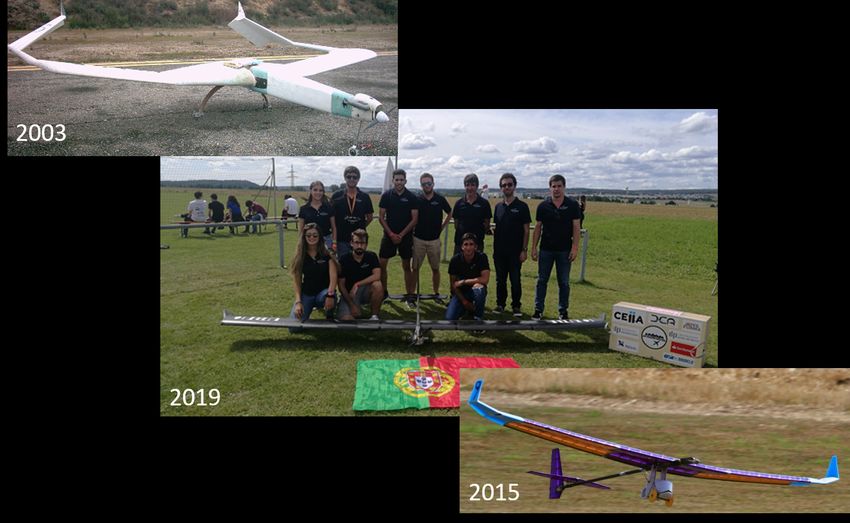
Figure 1.1: Some of UBI participations in the ACC in previous years.
When it comes to the propulsion system, past editions (see figure 1.1) of the competition had
a few different limitations that aimed to make the challenge as fair as possible. In the 1st
1edition with electrical motorization (held in Portugal, in 2007), only the motor model and
the maximum allowed current were defined. In the 2nd , a device was measuring the current
throughout the flight and if it exceed a certain value, the team would lose points. In the 3rd ,
an electronic device was installed on the aircraft in order to limit the throttle input. The 4th
edition was the first time that the propeller was pre-selected. For the 2021/2022 edition, the
goal is to build an electrical unmanned aircraft with the virtual task of transporting medical
goods. The motor is defined by the rules and the battery is limited to a 3S li-po. A choice
between two propellers is allowed. There is freedom to choose the electronic speed controller
(ESC) as long as it is commercially available, so one way of improving the performance of the
propulsion system is by optimizing the motor control, which will be the focus of the present
work.
1.2 Scope
This particular study aims to maximize the performance of the propulsion system by means
of ESC selection and its settings. The output power and generated thrust will be measured
in static condition and with relative wind for trapezoidal commutation and field-oriented
control (FOC). Field weakening implementation will also be studied as a mean of increasing
the thrust at high relative wind speed, given the 3S battery voltage limitation. The overall goal
is to find out what control strategy should be used to maximize the thrust available to the ACC
aircraft. Although it is directly targeted for this competition, the collected results should be
helpful for any systems that use brushless motors such as cars, skateboards, multi-copters,
etc. Since one of two different propellers may be used, they will also constitute one of the
variables of this study.
1.3 Objectives
• Understand how every parameter changed in the ESC affects the thrust produced and
current consumed by the set;
• Obtain static thrust and motor current consumption values for the different control
strategies and propellers;
• Characterize the thrust produced and current consumed as functions of relative wind
speed for the different control strategies and propellers;
• Find out what control strategy and propeller should be used in the ACC aircraft in order
to maximize its performance.
1.4 Document Structure
This dissertation has the following structure:
2• Chapter 2 presents a brief literature review starting by a summary of important con-
cepts regarding electric motors and their control as well as description of the state of
the art of motors and speed controllers;
• Chapter 3 documents the methodology that was followed in order to prepare the ESCs,
motor and propellers for the static and dynamic tests, as well as the procedures of the
tests themselves;
• Chapter 4 presents the results of the tests of the different propellers, ESCs and settings,
as well as a discussion of these results;
• Chapter 5 summarizes the conclusions and provides some recommendations for future
work.
34
Chapter 2

Literature Review

2.1    Fundamentals

2.1.1 Brushed DC Motor

As the name suggests, brushed motors make use of brushes. These are internal electrical
commutators that reverse the polarity of the active wire coils as they go through the magnets.

There are 3 main parts in a brushed motor: the stator, the rotor, and the commutator [2]. A
scheme of the general design is shown in figure 2.1.

                             Figure 2.1: Brushed DC Motor design [3].

The stator contains the permanent magnets. Instead, an electromagnet could be used in a
shunt, series or compound configuration, but they make it harder to maintain a magnetic
field in smaller motors. The permanent magnets are arranged in pairs of alternating north-
south, so there is always an even number of magnets in a motor.

The rotor contains the armature, which consists of windings of copper wire. When receiving
energy, half of the armature will have an electrically induced magnetic north pole that will
be attracted to the south poled permanent magnet, while the electrically induced magnetic
south pole armature will be attracted to the north poled permanent magnet. This will cause
the stator and rotor to rotate towards a state of equilibrium. As the motor approaches this
state, the commutator inverses the magnetic polarity of the armature, which forces it to keep
rotating towards the now new state of equilibrium. More coils of wire connected to more
segments of the commutator can be used in order to reduce the speed and torque fluctuation
and make the motor run more smoothly and efficiently.

                                              5
There are a few advantages and disadvantages of this type of motor [4]. They are cheaper and
easier to make in smaller sizes. There is also no need for an ESC, since the speed is controlled
via the bus DC voltage. The main disadvantage is the wear-out of the brushes. Another one
is that these motors create a lot of electromagnetic interference due to brush arcing, which
causes heat. At last, the inefficiency of this type of motor grows with speed, in part due to the
contact friction of the brushes.
2.1.2 Brushless DC Motor
A brushless motor is, as the name suggests, a motor without brushes. It is composed of a
stationary part, called the stator, which contains the copper windings and a rotating part,
called the rotor, which contains the permanent magnets [2]. As this type of electrical motor
does not make use of brushes or any other mechanical commutators in order to run, the
commutation has to be performed externally on a device called Electronic Speed Controller.
The most common configurations are axial-flux and radial-flux, with the radial-flux being
much more popular. In this category, there are inner-rotors and outer-rotors. In the inner-
rotors, the rotor is located in the inner side, while in the outer-rotors, the rotor is located in
the outer side of the motor. The differences can be seen in Figure 2.2. Inner-rotors usually
have a lower diameter, lower rotor inertia and high power due to high rotational velocity with
a limited torque. They are used in robotics, manufacturing and tools such as pumps, convey-
ors, compressors. Outer-rotors usually have a larger diameter and a larger rotor inertia and
torque production, which makes it better for constant speed applications such as fans, direct
drive machine tools and vehicle propulsion.
Figure 2.2: Radial-flux inrunner and outrunner diagram (adapted from [5]).
An individual group of windings that lead to a single terminal outside of the motor is called a
phase. The majority of brushless motors are 3-phased. A pole is a single permanent magnet
pole, north or south. In the figure above, each of the motors has 2 pairs of poles. At least a
pair of poles must exist and there is no theoretical limit for the number of pairs.
6The lack of brushes means that there is less friction, which allows brushless motors to operate
at higher speeds, have less heat production and overall higher efficiency. They also have
higher output power to size ration and last longer than the brushed motors. Although the
need for an external ESC makes this motor more costly and complex, the fast development
of technology almost eliminates this factor.
In electric motors, there is a difference between mechanical and electrical rotations or angles.
The mechanical angle is the physical angle that the rotor rotates relative to the stator, so a 360
degree rotation would mean that the rotor completed one revolution, which can be observed
directly. The electrical angle corresponds to the angular rotation of the flux and depends on
the number of poles the motor has. If a given motor has 1 pair of poles,Npoles , the electrical
rotation would equal the mechanical rotation, but if a motor has 2 pairs of poles, making
a rotation of 360 mechanical degrees, θmech , would mean that it completed 720 electrical
degrees, θelec , according to equation 2.1.
θelec = θmech .Npoles (2.1)
2.1.2.1 Theoretical Model
There are many models of electrical motors, ranging from simplistic to very complex ones.
Here, the first-order model of the DC electric motor [6] will be discussed, which quickly helps
to predict the behavior of a DC motor. Figure 2.3 shows the circuit that is equivalent to a DC
motor.
Figure 2.3: Equivalent circuit for a DC electric motor [6].
R is the resistance at the terminals of the motor and is assumed constant.
Qm is the shaft torque and is assumed to be proportional to the current i via KQ , the torque
constant, minus a friction torque loss related current io .
Qm (i) = (i − io )/KQ (2.2)
vm is the internal back electromotive force (BEMF) and is assumed to be proportional to the
7mechanical angle velocity Ω via KV , the motor speed constant.
vm (Ω) = Ω/KV (2.3)
The motor terminal voltage is then obtained by adding on the resistive voltage drop.
v(i, Ω) = vm (Ω) + iR = Ω/KV + iR (2.4)
We can now manipulate this equations to obtain current, torque, power and efficiency values,
as functions of the motor speed and voltage at its terminals.
Ω 1
i(Ω, v) = (v − ) (2.5)
KV R
1 Ω 1 1
Qm (Ω, v) = [i(Ω, v) − io ] = [(v − ) − io ] (2.6)
KQ KV R KQ
Pshaf t = Qm Ω (2.7)
PShaf t i o KV 1
ηm (Ω, v) = = (1 − ) (2.8)
iv i KQ 1 + iRKV /Ω
In the case of zero friction (io = 0) and zero resistive losses (R = 0), the equation of efficiency
(2.8) becomes
KV
ηm = (2.9)
KQ
So, for energy to be conserved, the torque constant KQ must be equal to the speed constant
KV . In these equations KV is in rad/s/V and KQ is in the equivalent unit of A/Nm. However,
KV is usually presented in revolutions-per-minute/V (RPM/V).
The motor speed constant is an important value for brushless motors and it is always pro-
vided by the motor manufacturers. It corresponds to the number of RPM that a motor makes,
for each Volt that is applied to it, with no load attached. By knowing this value, it is possible
to quickly find out how fast the motor rotates for a given battery or power supply.
82.1.2.2 Motor Parameter Measurement
• Motor Resistance
The motor resistance R can be obtained by using a multimeter (or ohmmeter) to mea-
sure the resistance, although usually the values are too that so an accurate value is hard
to obtain. Alternatively, a current i can be fed across two terminals of the motor, while
measuring the voltage v across it. Then, resistance R can be calculated from Ohm’s
Law (2.10).
R = v/i (2.10)
• Zero-load Current
Zero-load current, io can be measured by applying a voltage v to the motor, and then
running it at full throttle, with nothing connected to its shaft. For the typical brushless
outrunner motor used in the Air Cargo Challenge UAV size class, a 10 V power supply is
usually used. Although the simple motor model considers constant friction torque, in
reality, a higher angular velocity normally results in a higher friction torque. Therefore,
the specification of io of the motor is typically followed by the voltage used for that test.
• Speed Constant
The speed constant can be computed from (2.3):
Ω
KV = (2.11)
vm
where vm , the back-EMF voltage, can be calculated with the previously obtained resis-
tance R, voltage v and zero-load current io .
v m = v − io R (2.12)
• Torque Constant
The Torque Constant KQ can be obtained from motor torque data. According to torque
model (2.2), Qm plotted against i − io is a straight line crossing the origin. The slope
1
of this line then gives KQ . As can be observed from (2.9), any difference between KQ
and KV will result in an efficiency lower than 1, and may be an indicative of the im-
perfections of this motor model. Alternatively, KQ may simply be assumed equal to
KV .
92.1.3 Brushless Speed Control
As brushless motors do not have a commutator, a dedicated external speed controller is
needed. These electronic speed controllers, usually take a DC power input and a Pulse-Width
Modulation (PWM) duty cycle input signal and output a voltage and current for each phase of
the motor as functions of the motor electrical angle position, in order to keep it a certain op-
erating condition [7]. The phase current should ideally replicate the motor’s BEMF, which
is discussed in subsection 2.1.4. The more basic controllers apply voltage over two of the
three phases of the motor, which creates an electromagnetic field around them. As the per-
manent magnets are attracted or repelled by this electromagnetic field, they cause the rotor
to move. The controller then switches the phases and the magnets are attracted to another
electromagnetic field. As long as this electronic phase shifting keeps happening, the rotor
will keep chasing the electromagnetic field created by the stator and the motor will keep run-
ning. More advanced controllers can power the 3 phases simultaneously. This allows for a
more efficient and smoother operation of the motor, at the expense of higher ESC complexity
and computational cost.
There are 3 main parts to an ESC: the position sensing, the processor, and the gates (also
called inverters). The first one is responsible for reading the motor’s electrical position,
which can be achieved with or without position sensors. The processor takes the input from
the first one as well as input from the user to calculate when and which gates should be
switched. The gates are responsible for connecting or disconnecting a given motor termi-
nal to or from the DC supply. For this, electronic power switches are used. They are usually
MOSFETs (Metal–Oxide–Semiconductor Field-effect Transistors) or IGBTs (Insulated-Gate
Bipolar Transistors). The MOSFETs resistance is constant, so the voltage drop across its ter-
minals increases with current, while the IGBTs voltage drop remains constant because the
resistance changes with current. Thus, the first ones are usually used with lower power ap-
plications because that is when they have less resistance, while the latter ones are used in
systems with higher voltages [8].
2.1.4 BEMF
As the motor rotates, it induces a counter-electromotive force on the motor phases due to
magnetic induction [8], following Faraday’s law. For instance, when a motor is disconnected
from a power source and connected to an oscilloscope, rotating the motor manually will pro-
duce a BEMF that can be measured. This voltage is a function of the electrical position angle
of the rotor and its magnitude is proportional to the angular velocity of the motor, so by
measuring it, the angular velocity of the motor can be determined.
Depending on the shape of their BEMF, brushless motors can be differentiated into two
types: BLDC and PMSM. BLDC motors characteristically have a more trapezoidal BEMF,
while PMSM motors have a more sinusoidal BEMF. Figure 2.4 shows the ideal trapezoidal
and sinusoidal BEMF waves, normalized to root mean square (RMS) of 1.
10Magnet and stator core geometry, magnetization and winding distribution are some proper-
ties of the motor design that affect the shape of the BEMF [9].
The working principle of both BLDC and PMSM is the same. The difference is that in a
PMSM, the coils of the stator are wound in a sinusoidal manner.
Figure 2.4: Ideal sinusoidal vs. trapezoidal back EMF waveforms, normalized to RMS=1 [9].
2.1.5 Sensored and Sensorless Control
2.1.5.1 Sensored
The simplest way of knowing the electrical position of the motor rotor is by using a position
sensor. This type of sensor sends information about the position of the motor rotor to the
controller, which then uses it to drive the motor in the most effective way. The most common
devices for this are Hall effect sensors and magnetic or optical encoders [10].
When using sensors, the motor is able to rotate more smoothly and with more torque right
from zero RPM, thus this type of motor is used when low constant speeds or high position
precision is needed, for example, in drills or camera gimbals.
2.1.5.2 Sensorless
Sensorless motor control can be performed through flux measurement or BEMF wave detec-
tion methods [11]. The first one is more complicated and more costly in terms of hardware
and processing, thus BEMF detection methods are usually preferred commercially and in-
dustrially [12]. Since the motor does not generate any BEMF at zero RPM, it has to be rotating
at a minimum speed in order to generate BEMF that allows to apply these methods. So, at
zero RPM, the ESC drives the motor in open-loop [13], which means that it tries to rotate the
motor without feedback. This sometimes results in jerking of the motor which is not seen
11in sensored control. Once the motor is running at a sufficient speed, the generated BEMF
allows the algorithm in the controller to estimate the rotor position and drive the motor in
a closed-loop. Although sensorless control is not very good at low speeds, it performs really
well at high speeds, which is one of its advantages over the sensored control. It is also lighter
but requires more computational power. This type of control is used a lot in radio-controlled
(RC) model aircraft and Air Cargo Challenge sized UAVs, because they tend to operate at
higher speeds and the starting torque needed to rotate the propeller is very low.
122.1.6 Motor Control - Trapezoidal, Sinusoidal and FOC
2.1.6.1 Trapezoidal
With this method, one of the three motor terminals is off at any time, the other is sinking
current, and the last one is sourcing current. For this, and in the same order, one of the
phases is un-energized, the other is connected to the positive DC power supply terminal,
and the last one is connected to the negative DC power supply terminal [14]. This generates
a magnetic field in the stator, which interacts with the magnets and makes the rotor spin.
Recurring to position sensors or BEMF sensing, the controller switches the phases in order
to keep it spinning. Figure 2.5 illustrates the behavior of trapezoidal motor control. The hall
sensor output can be seen, as well as the BEMF, the torque the motor outputs and the phase
current shifting.
Figure 2.5: Hall sensor signal, BEMF, output torque and phase current waveforms of an electrical motor with
trapezoidal BEMF as function of electrical position angle (adapted from [15]).
The resulting waveform is almost of trapezoidal shape, depending on the motor inductance.
Simplicity and cost effectiveness are the main advantages of this type of control, but it also
has some disadvantages, such as torque ripple.
132.1.6.2 Sinusoidal
Sinusoidal commutation is used in motors with a sinusoidal back EMF, which are considered
AC motors. In this type of commutation, current is injected simultaneously in all the phases
of the motor (see table 2.1) in the form of sine waves. In reality, these waves are generated
with high frequency PWM square waves, which then, with the inductance of the motor, are
filtered into sinusoidals. For this type of commutation, a high resolution position sensor such
as an encoder is recommended, which is why this is a more expensive solution. Although it
reduces the torque ripple and noise that is present in the trapezoidal commutation, sinusoidal
commutation is not as good as trapezoidal beyond a certain electrical speed. In the case of the
ACC motor-propeller setup, the electrical speed is high enough to allow sensorless sinusoidal
control, but possibly low enough to still have an efficient control compared to the trapezoidal
ESC.
Motor Position Inverter State
Interval (degrees) Hall A Hall B Hall C ON Switches Phase A Phase B Phase C
0 to 60 1 0 1 S1, S6, S5 + - +
60 to 120 1 0 0 S1, S6, S2 + - -
120 to 180 1 1 0 S1, S3, S2 + + -
180 to 240 0 1 0 S4, S3, S2 - + -
240 to 300 0 1 1 S4, S3, S5 - + +
300 to 360 0 0 1 S4, S6, S5 - - +
Table 2.1: Switching sequence for sinusoidal commutation [8].
PWM is a way of controlling the current delivered to the phases of the motor by turning the
circuit on and off in pulses of different duration. Consider a load where the power supply is
on during half of the considered time frame and off during the other half. The mean current
level would be half of the state where the power supply is on during the whole period. Thus,
the current level is proportional to the on time-fraction.
Figure 2.6 exemplifies how a sinusoidal current can be generated using square PWM waves.
In this circuit, a comparator is fed with a reference sinusoidal wave signal, Ursw , in the pos-
itive terminal that is compared with a triangular wave signal in the negative terminal, Utw .
When Ursw > Utw , SA = 1 , which generates a pulse to the gates driver. During the duration
of the pulse, the upper left gate and lower right gate close the circuit, applying +VDC to the
phase A of the motor. During this condition, IA increases in time with an increase rate pro-
portional to the motor inductance. When Ursw < Utw , -VDC is applied to the phase A of the
motor, making IA decrease in time. This results in a sinusoidal current with a small amount
of ripple, due to the motor inductance.
14Figure 2.6: Sinusoidal wave generation with PWM [8].
2.1.6.3 Field-Oriented Control
Field-oriented control is a more advanced technique that transforms the 3 phase currents in
2 separately controlled components: torque and flux [16]. First, the 3 phase sinusoidal cur-
rents (Ia , Ib , Ic ) are transformed into a two-phase (α, β) system that varies in time through
the Clarke transformation. Then, α and β are transformed into the d,q reference frame us-
ing the Park’s transformation. In this two-coordinate time invariant system, the direct-axis
represents the flux, which depends on the rotor’s electrical position, and the quadrature-axis
represents the torque, which depends on the current, and is 90º apart from the d-axis [17].
At this point, and according to the torque necessary, d and q can be adjusted. The d-axis has
a magnetising or demagnetising effect on the motor, so this component is usually required
to be zero in order to maximize the motor’s torque (q-axis) and efficiency.
After the d and q values are defined, they are transformed back into the stationary reference
frame through the inverse Park’s and Clarke’s transformation, resulting in the time depen-
dent 3-phase currents. The output of the inverse Clarke transformation provides the duty
cycles of the PWM channels corresponding to the three phase voltages. Space Vector Modu-
lation may then be used or not, depending on the chosen control algorithm [18]. These steps
are illustrated in Figure 2.7.
15This type of control is much more demanding on the hardware, thus requiring more complex
and expensive components.
Figure 2.7: Field-oriented control structure.
Table 2.2 shows the main similarities and differences between the 3 commutation methods
discussed above.
Technique Trapezoidal Sinusoidal FOC
High starting torque, Lower but
Start-Up Power Lower starting Torque
but lots of ripple smoother starting torque
Power Delivery High torque ripple Smooth Smooth
Speed Control Excellent Excellent Excellent
High Speed Performance Good Poor Excellent
Controller Complexity Low Medium High
Table 2.2: Commutation Methods Comparison (adapted from [19]).
2.1.7 Field Weakening
As established earlier, when a motor rotates, it creates a back EMF voltage that is propor-
tional to the speed of rotation. In order to push current into the coils, the supplied voltage
must be greater than this BEMF voltage. The limit is reached when the speed is such that
the BEMF voltage is the same as the supplied voltage, and the inverter can no longer push
current into the stator coils. This means that for a given voltage supply, there is a maximum
rotational speed for a given motor: the base speed [20].
16In order to exceed this speed, the BEMF voltage needs to be reduced, and this can be achieved
by forcing negative current to the d axis of the motor, which causes the rotor magnets mag-
netic flux to be reduced, and lowers the BEMF. With this, it is possible to achieve higher
rotational speeds. On the other hand, torque is proportional to field flux, so, while the ro-
tational speed is increased, the torque is reduced, thus, requiring more current to reach the
same motor torque. Therefore, the motor efficiency is reduced.
This region is shown in Figure 2.8, where the maximum torque, maximum power and maxi-
mum rotor flux are plotted. Only the shape of the plots should be considered. This effect can
be seen as an increase of the KV of the motor, in exchange for efficiency.
Figure 2.8: Field weakening region (adapted from [21]).
2.2 State of the Art
There are many recent studies that aimed to add something new and better to the motor
control strategies discussed earlier. On the other hand, no studies were found regarding the
influence of the control strategy on the performance of a motor-propeller system and how
it would relate with the actual performance of the aircraft. Trapezoidal commutation is still
very much in use, but it is becoming outdated, which is why the most recent studies tend
to focus on FOC, which is becoming the standard as the technology evolves. The studies
mentioned next are mainly related to FOC and field weakening, because these are areas that
still need to be studied and continue to have room for improvement.
Alessandro Bosso et al [22], documented his work in developing a computationally-effective
17field-oriented control strategy by integrating a recent sensorless observer into the system,
without requiring any information of the mechanical dynamics and their parameters.
Micael Ratcliffe and Kelum Gamage [19] from Lancaster University proposed a new power
control technique that aimed at reducing switching losses by centering the driving current
around the optimum flux interaction point and bringing the PWM frequency down to that of
the commutation frequency.
Hastanto Widodo et al [23], proposed a novel electronic speed controller with rotor field
control in addition to standard motor power control. In order to approach the ideal BLDC
motor concept, an automotive generator was converted into a BLDC motor. Unlike a normal
BLDC motor, which has a standard power curve characterized with maximum power which
is only achievable in one specific speed, the proposed setup could allow the motor to have an
adjustable maximum power in a wide range of operation speeds.
The physical components present in the ESC also affect its performance. Part of the study
made by Young Tae Shin and Ying-Khai Teh [24] focused on how the type of power transistor
would affect the overall efficiency of a small commercial quadcopter UAV. They compared
a few models of transistors with Si-IGBT (Silicon-based Insulated Gate Bipolar Transistor),
SiC (Silicon Carbide Semiconductor) and GaN (Gallium Nitride Semiconductor) technology
and translated that to the flight time that a specific drone would have if using each.
The effect of field weakening can also be improved by designing the motor for that purpose.
Senol and Uston [25] developed a BLDC motor with higher direct-axis phase inductance,
which provided a better performance in the field weakening region.
The literature survey allowed to conclude that the the present work is a novelty in the electric
aircraft motor control field, given that there were not found any similar studies on control
methods or field weakening effects on the performance of a propeller aircraft.
18Chapter 3
Methodology
3.1 Motor
The motor used was defined by the Air Cargo Challenge rules: the AXI 2826/10. This is a
PMSM outrunner type of motor, with 7 pairs of poles in the rotor. At the time of the real-
ization of this study, there were 2 available options, the AXI 2826/10 GOLD LINE and the
newer AXI 2826/10 GOLD LINE V2. A picture and a technical drawing of each is shown in
Figure 3.1.
Figure 3.1: On the left: AXI 2826/10 GOLD LINE, on the right:AXI 2826/10 GOLD LINE V2 [26]
The specification of each motor are shown in Table 3.1.
19AXI 2826/10 GOLD LINE AXI 2826/10 GOLD LINE V2
Battery 3 - 5 Li-Poly 3 - 5 Li-Poly
RPM/V 920 920
Max. efficiency 84% 86%
Max. efficiency current 20 - 30 A (>78%) 20 - 30 A (>78%)
No load current 1.7 A 1.7 A
Current capacity 42 A/60 s 43 A/60 s
Internal Resistance 42 mohm 20 mohm
Dimensions (D x L) 35x48 mm 35x52 mm
Shaft diameter 5 mm 5 mm
Weight 181 g 177 g
Max. Power 723 W 740 W
Table 3.1: AXI 2826/10 GOLD LINE and AXI 2826/10 GOLD LINE V2 specifications [26].
Right off the top, the V2 has a 2% more maximum efficiency, that although is not very relevant
for the goal of this study, shows that the construction of the motor has been upgraded. It can
now handle 1 more Ampere of maximum current, increasing the maximum power to 740W.
The internal resistance has also been reduced by more than 50% and thermal properties have
been enhanced, which is important because field weakening may heat up the motor. With
all these improvements, plus a reduction in weight, the V2 appears to be a better choice, and
the tests were conducted with it.
The BEMF of the ACC motor was measured using an oscilloscope. It can be observed in
Figure 3.2 that the BEMF of this motor has a more sinusoidal shape, rather than trapezoidal.
The measured BEMF is represented in blue, and a sinusoidal wave was added in a yellow
dashed line for comparison reasons.
Figure 3.2: Measured BEMF of the ACC motor (in blue).
203.2 Electronic Speed Controllers
When it comes to the ESCs, 2 of them were used. One was the Castle Creations Phoenix ICE
75 (CL PI 75), which uses sensorless trapezoidal commutation to drive the motor, and the
other one was an A50s by Team Triforce UK, which runs VESC software and supports field-
oriented control, and, more recently, field weakening. A picture of both is shown in Figure
3.3.
Figure 3.3: On top: Castle Creations Phoenix ICE 75, on bottom: Team Triforce UK A50S
Characteristics of the Castle Creations Phoenix ICE 75 include:
• Current Rating: 75 A;
• Voltage Rating: Li-Po 1S - 8S and Ni-Cd/Ni-MH 1S-22S;
• Mass with wires: 99 g;
• Dimensions without wires: 66 x 33 x 22.9 mm3 ;
• Selectable BEC: 5 A max, 5-7 V (in increments of 0.1 V);
This ESC was selected to represent the trapezoidal strategy, due to Castle Link being a rep-
utable brand that produces high quality ESCs.
Characteristics of the Triforce A50S include:
• Current Rating: 23 A with no airflow, 35 A with light airflow, 50 A burst;
• Voltage Rating: Li-Po 2S - 6S;
• Mass with wires: 19 g;
• Dimensions without wires: 34.2 x 17.9 x 5.5 mm3 ;
• BEC: 5 V, max 0.4 A;
This ESC was selected to represent the FOC strategy because it supported VESC software and
21field weakening, and is much smaller compared to similar devices.
Between the chosen ESCs, the size difference is significant and has great impact on the cool-
ing of the ESC. The Phoenix ICE 75 has its size mainly because of the included heat sink. The
Triforce A50S lacks this heat sink, which made it heat up quite a bit when field weakening
was enabled. The solution implemented in the static and dynamics tests were different and
are discussed in the sections 3.3 and 3.4. A more definitive solution is presented in chapter
5.
To switch efficiently between ESCs, bullet connectors were soldered to the ESC and motor
leads, as well as XT60 connectors for connection with the power supply. Figure 3.4 shows
the connection diagram of the components.
Figure 3.4: Connection diagram of the static test setup.
3.2.1 Castle Creations Phoenix ICE 75
In order to connect this ESC to a computer, a Castle Link adapter and the Castle Link software
are needed. All the options in the program are presented in drop down menus along with
their meanings, which are thoroughly explained and make it very simple to use.
The settings that were changed in this study to see its impact on performance were Motor
Timing and PWM Rate (see Figure 3.5).
In Motor Timing Advance three options are provided: Low, Normal and High. This setting
changes the timing advance range used on the motor. In other words, it is going to send
current to the motor earlier or later, depending on the chosen option, which makes the motor
receive the current more or less in phase with the its BEMF. If the current is in phase with
the BEMF, all current will be used for torque production, the motor will be more efficient
and no field weakening will take place. Normally, the Low setting is slightly more efficient
and provides less power, while the High setting makes the current advance in relation to the
back electromotive force, thus providing some field weakening, so it is slightly less efficient
and provides more power.
22Changing the PWM Rate changes the frequency at which the ESC sends commands to the
motor. In theory, using higher frequencies, the motor RPM can be controlled more accurately
but it also increases the temperature of the controller.
Figure 3.5: Screenshot of Castle Link showing some the settings that were changed in this study.
3.2.2 Triforce A50S
In order to connect the Triforce A50S ESC to the computer, a USB to micro USB cable is
needed and the ESC must be powered externally. VESC Tool [27] must also be installed on
the computer.
VESC Tool is a feature packed software that works with VESC ESCs such as the Triforce A50S.
The software allows to upload firmware to the ESC, monitor and control a large a number of
settings such as temperature, voltage, current and RPM ranges, PID control, position sens-
ing, commutation modes, etc. It can also receive real-time data from the ESC or conduct
automated runs.
To begin using the program, the connection to the ESC must be made by clicking on Auto-
Connect (see number 1 in Figure 3.6). If the motor and ESC combination is being used for
the first time, the “Setup Motors FOC” (see number 2 in Figure 3.6) wizard should be ran, so
that the ESC can detect the following motor parameters: Motor Resistance (R) in Ohm [Ω],
Motor Inductance (L) in Henry [H] and Motor Flux Linkage (λ) in Weber [Wb].
Next, the FOC optimization on the bottom of the FOC page should be ran in order to optimize
the motor control.
At this point, the motor is ready to spin. Manual adjustments to settings such as maximum
motor currents, maximum battery currents, RPM limits, etc. may be made if needed. When-
ever making any changes, the ”write motor configuration” (shown in Figure 3.6) button on
the right side toolbar has to be clicked so that the information is sent to the ESC. Similarly,
23the ”read motor configuration” (see Figure 3.6) button can be used to read what information
is written on the ESC.
Figure 3.6: Screenshot showing the welcome page, the AutoConnect button and the Setup Motors FOC button.
For this study the switching frequency was first changed, but the motor would not run as
smoothly as in the default 25 kHz value, so the changes were reverted and the frequency
remained the same throughout the experiments.
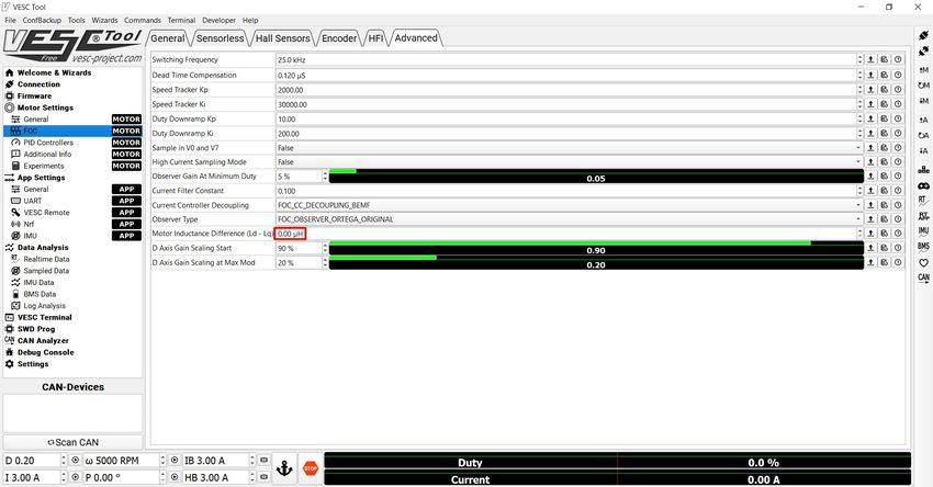
The parameter changed next was the one responsible for field weakening. In this tool, it is
presented as a ”Motor Inductance Difference (Ld − Lq)” [μH] (see Figure 3.7). In order to
have this option, the ESC must be updated to the latest firmware, which was provided by
Team Triforce following our e-mail request. The difference between Ld and Lq inductance
represents the motor saliency. A value different from zero will enable field weakening, which
will gradually inject negative current in the field axis as throttle increases, weakening the
magnets of the motor.
24Figure 3.7: Screenshot of the VESC Tool, on the page where Field Weakening may be enabled (in the red box).
253.3 Static Tests
Static tests provide an insight on the behaviour of the chosen setup on the ground, where
there is little to none relative wind. The static tests were conducted in the Faculty of Engi-
neering of University of Beira Interior. A diagram of the static thrust measuring stand setup
is shown in Figure 3.8.
Figure 3.8: Diagram of the static thrust measuring stand setup.
A rocker made of two wooden levers at a 90º angle, connected with 3D printed pieces and
ball bearings make it possible to transfer the thrust produced by the propeller to the scale.
Although the wooden poles have the same length, the important measurements to take into
consideration are the distance from the ball bearing axis to the motor and propeller axis
(represented by H in Figure 3.8) and the distance from the ball bearing axis to the touching
point in the scale (represented by L in Figure 3.8). In this case, H was 22.5 cm, and L was
24 cm. So in order to obtain the correct values, the value read on the scale was multiplied by
L/H.
A picture of the implemented setup is shown in Figure 3.9.
26Figure 3.9: Picture of the static thrust measuring stand setup.
The ESC and motor were powered with a power supply set to 12.00 V and a current rating of
up to 60 A. The voltage was set to 12.00 V because it is representative of the battery of the
aircraft in the take-off stage of the Air Cargo Challenge. A multimeter with a Hall effect clamp
and a precision of 0.1 A was used to measure the current and a SF-400A kitchen scale with
a precision of 1 g was used to measure the thrust. It is important to note that when enabling
field weakening, the Trifoce A50S heated pretty fast, so it was mounted in the prop wash of
the propeller in order to keep it at a safe temperature (as seen in Figure 3.9)
It is also important to keep in mind not to use cables that are too long from the power supply
to the ESC, because their inductance increases with length and this was the reason why on
the first static tests the ESC would shut down at high currents.
3.3.1 Testing Conditions
Each test consisted of an incremental increase of throttle from roughly 10% to 100%. The
Triforce A50S was controlled directly from the computer via the VESC Tool. So, it was possi-
ble to know at what throttle percentage it was at all times. Since the Phoenix ICE 75 did not
have this feature and it was being controlled with a servo tester, the throttle was gradually
increased and after each run, the ESC log file was read to know the exact throttle percentage
that corresponded to each thrust and current values.
With the Phoenix ICE 75, 9 tests were conducted with each propeller, corresponding to 9
different combinations of PWM Rate and Motor Timing, as shown in Figure 3.10.
27Figure 3.10: Static tests performed with the Phoenix ICE 75 ESC.
With the Triforce A50S, 4 tests with each propeller were performed, corresponding to differ-
ent magnitudes of field weakening, as shown in Figure 3.11.
Figure 3.11: Static tests performed with the Triforce A50S ESC.
This resulted in 26 different testing conditions for the static experiments. The results are
shown in Section 1 of Chapter 4.
283.4 Wind Tunnel Tests
Wind tunnel tests provide an overview of how the chosen setup behaves in flight, where there
is relative wind.
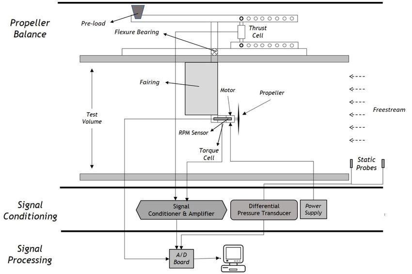
The main wind tunnel in University of Beira Interior was used. Its installation is thoroughly
documented in [28]. A general scheme is shown in Figure 3.12.
Figure 3.12: Measurement System Schematic Overview (adapted from [28]).
This tunnel is equipped with various equipment such as an RPM Sensor that outputs the
RPM of the motor, a torque cell used to measure the torque generated by the motor, and
a load cell to measure how much thrust is generated. The freestream velocity is measured
with a differential pressure transducer, an absolute pressure transducer and a thermocou-
ple. A mast fairing is also installed over the wiring and motor fixation structure to make it
more aerodynamic. A pre-load is placed on the opposite side of the load cell responsible for
measuring thrust, in order to keep it in tension even during negative thrust conditions.
Figure 3.13 shows a picture of the installation.
29Figure 3.13: Picture of the wind tunnel setup mounted with the Aeronaut 10x6 propeller.
Figure 3.14: Flowchart of the test methodology used in the wind tunnel.
30The tunnel is equipped with its own ESC that is directly connected to the LabView software
on the computer and it is usually used to test motors and propeller. As it was needed to use
different ESCs, the tunnel ESC was disconnected, thus losing the motor connection to the
LabView software, which is not relevant since the tests were performed at full throttle. The
procedure is described in the flowchart in Figure 3.14.
Before starting the experiments, full calibration of the torque sensor, the load cell and pres-
sure sensors were made. Every test was performed at open throttle and with an incremental
increase of the wind speed, starting at 5 m/s and up to a maximum of 32 m/s, depending
on how much thrust was being generated, so that windmill break state would be avoided.
At each wind speed, and after convergence, a 200 point average of the measured values was
calculated and stored automatically by the LabView software.
The uncertainties of the primary measurement sensors are displayed in Table 3.2. The un-
certainty of the measured results is shown in subsection 4.2.5 and was calculated using the
methodology described in reference [29].
Measurement Sensor Uncertainty
Thrust, T FGP FN3148 ∆T = ±0.05N
Torque, Q Transducer Techniques RTS-100 ∆Q = ±0.000339N.m
Atmospheric Temperature, Tatm National Instruments LM335 ∆Tatm = ±1.0K
Atmospheric Pressure, Patm Freescale Semiconductor MPXA4115A ∆Patm = ±30.0P a
Propeller Rotation Speed, n Fairchild Semiconductor QRD1114 ∆RP M = ±5RP M
Static Ports Differential
MKS 226A ∆(p1 − p2 ) = ±0.003xReading
Pressure, (p1 − p2 )
Table 3.2: Uncertainties of the primary measurement sensors.
The measured values are: thrust (T ), torque (Q), freestream velocity (V ), revolutions per
second (n), voltage (v), current (I), static pressure (Ps ), atmospheric pressure (Patm ) and air
temperature (Tatm ).
From these quantities, the air density ρ can be computed:
Patm
ρ= (3.1)
RTatm
Advance ratio, J, can be calculated with V , n and the propeller diameter, D:
V
J= (3.2)
nD
Thrust coefficient, CT , and power coefficient, CP are calculated with the respective parame-
ters T and power, P = 2πnQ.
31You can also read