Technical note: The CAMS greenhouse gas reanalysis from 2003 to 2020
←
→
Page content transcription
If your browser does not render page correctly, please read the page content below

Technical note
Atmos. Chem. Phys., 23, 3829–3859, 2023
https://doi.org/10.5194/acp-23-3829-2023
© Author(s) 2023. This work is distributed under
the Creative Commons Attribution 4.0 License.

                        Technical note: The CAMS greenhouse gas
                               reanalysis from 2003 to 2020
       Anna Agustí-Panareda1 , Jérôme Barré2 , Sébastien Massart1 , Antje Inness1 , Ilse Aben3 , Melanie Ades1 ,
        Bianca C. Baier4,5 , Gianpaolo Balsamo1 , Tobias Borsdorff3 , Nicolas Bousserez1 , Souhail Boussetta1 ,
            Michael Buchwitz6 , Luca Cantarello1 , Cyril Crevoisier7 , Richard Engelen1 , Henk Eskes8 ,
          Johannes Flemming1 , Sébastien Garrigues1 , Otto Hasekamp3 , Vincent Huijnen8 , Luke Jones1 ,
        Zak Kipling1 , Bavo Langerock9 , Joe McNorton1 , Nicolas Meilhac7 , Stefan Noël6 , Mark Parrington1 ,
         Vincent-Henri Peuch1 , Michel Ramonet10 , Miha Razinger1 , Maximilian Reuter6 , Roberto Ribas1 ,
                    Martin Suttie1 , Colm Sweeney5 , Jérôme Tarniewicz10 , and Lianghai Wu11
       1 European   Centre for Medium Range Weather Forecasts, Shinfield Park, Reading RG2 9AX, United Kingdom
              2 Joint Center for Satellite Data Assimilation, University Corporation for Atmospheric Research,
                                                         Boulder, CO, USA
                           3 SRON Netherlands Institute for Space Research, Utrecht, the Netherlands
                                 4 Cooperative Institute for Research in Environmental Sciences,

                                        University of Colorado Boulder, Boulder, CO, USA
                                    5 NOAA, Global Monitoring Laboratory, Boulder, CO, USA
                 6 Institute of Environmental Physics (IUP), University of Bremen, 28334 Bremen, Germany
                                 7 Laboratoire de Météorologie Dynamique (LMD/IPSL), CNRS,

                                       Ecole polytechnique, 91128 Palaiseau CEDEX, France
            8 Royal Netherlands Meteorological Institute, Utrechtseweg 297, 3731 GA De Bilt, the Netherlands
                   9 Royal Belgian Institute for Space Aeronomy, Avenue Circulaire 3, 1180 Uccle, Belgium
              10 Laboratoire des Sciences du Climat et de l’Environnement (LSCE-IPSL), CEA-CNRS-UVSQ,

                                       Université Paris-Saclay, 91191 Gif-sur-Yvette, France
                         11 Remote Sensing Unit, Flemish Institute for Technological Research (VITO),

                                                Boeretang 200, 2400 Mol, Belgium
                         Correspondence: Anna Agustí-Panareda (anna.agusti-panareda@ecmwf.int)

                                      Received: 30 April 2022 – Discussion started: 18 July 2022
                         Revised: 26 January 2023 – Accepted: 16 February 2023 – Published: 31 March 2023

      Abstract. The Copernicus Atmosphere Monitoring Service (CAMS) has recently produced a greenhouse gas
      reanalysis (version egg4) that covers almost 2 decades from 2003 to 2020 and which will be extended in the
      future. This reanalysis dataset includes carbon dioxide (CO2 ) and methane (CH4 ). The reanalysis procedure
      combines model data with satellite data into a globally complete and consistent dataset using the European
      Centre for Medium-Range Weather Forecasts’ Integrated Forecasting System (IFS). This dataset has been care-
      fully evaluated against independent observations to ensure validity and to point out deficiencies to the user. The
      greenhouse gas reanalysis can be used to examine the impact of atmospheric greenhouse gas concentrations
      on climate change (such as global and regional climate radiative forcing), assess intercontinental transport, and
      serve as boundary conditions for regional simulations, among other applications and scientific uses. The caveats
      associated with changes in assimilated observations and fixed underlying emissions are highlighted, as is their
      impact on the estimation of trends and annual growth rates of these long-lived greenhouse gases.

Published by Copernicus Publications on behalf of the European Geosciences Union.
3830                  A. Agustí-Panareda et al.: Technical note: The CAMS greenhouse gas reanalysis from 2003 to 2020

1   Introduction                                                   range of scales from hours to seasons and from local to global
                                                                   scales (Agustí-Panareda et al., 2022).
Atmospheric carbon dioxide (CO2 ) and methane (CH4 ) are              Figure 1 showcases the global evolution of CO2 and CH4
the most abundant anthropogenic greenhouse gases directly          represented by the CAMS GHG reanalysis dataset over the
responsible for climate change (IPCC, 2021). Their long life-      period 2003–2020 and the span of the used satellite data. The
time and increasing anthropogenic emissions near the sur-          seasonal averages illustrate the spatial and temporal variabil-
face account for their long-term trends (Friedlingstein et al.,    ity information contained in the reanalysis dataset that can
2022). A lot of effort has been devoted to measuring the           be exploited for a range of applications in atmospheric sci-
atmospheric concentrations from ground-based observato-            ences. A key potential use of the CAMS GHG reanalysis is
ries, e.g. the National Oceanic and Atmospheric Adminis-           to assess the impact of greenhouse gases on climate change.
tration (NOAA, https://gml.noaa.gov, last access: 18 March         The reanalysis three-dimensional fields could be used to
2023) and the Integrated Carbon Observation System (ICOS,          investigate global and regional climate radiative forcing
https://www.icos-cp.eu, last access: 18 March 2023), which         (e.g. https://atmosphere.copernicus.eu/climate-forcing, last
provide the gold standard for the estimation of trends, and        access: 18 March 2023), serve as boundary conditions for
more recently satellite data (Committee on Earth Observa-          regional simulations, assess intercontinental transport, and
tion Satellites, CEOS; Crisp et al., 2018), enhancing the spa-     generally provide a reference for any other study focusing
tial coverage of greenhouse gas observations at the global         on atmospheric variability of CO2 and CH4 . However, care
scale. Atmospheric measurements also sample the variabil-          should be taken when using the CAMS GHG reanalysis to
ity of CO2 and CH4 coming from the weather and its as-             estimate trends and annual growth rates of these long-lived
sociated atmospheric transport (e.g. Patra et al., 2008, 2011).    greenhouse gases by considering the caveats associated with
For this reason, numerical weather prediction (NWP) models         the changes in the satellite retrievals of CO2 and CH4 and the
have been extensively used to represent and reconstruct the        fact that neither anthropogenic emissions nor natural fluxes
variability of atmospheric concentrations of various tracers       are adjusted by the data assimilation system, unlike atmo-
(e.g. Inness et al., 2019). Here we use the Integrated Forecast-   spheric inversions (e.g. Chevallier et al., 2019).
ing System (IFS) of the European Centre for Medium-Range              The objective of this technical report is to document the
Weather Forecasts (ECMWF), which has been adapted to in-           technical aspects of the method and input data used to pro-
clude CO2 and CH4 in the weather forecast (Agustí-Panareda         duce the CAMS GHG reanalysis and to provide guidance to
et al., 2017, 2019), to create a greenhouse gas (GHG) re-          potential users on the strengths and limitations of the dataset.
analysis. The reanalysis uses the data assimilation technique      Section 2 describes the processing chain to produce the re-
to combine CO2 and CH4 satellite data from the SCanning            analysis and its components. Section 3 focuses on the evalu-
Imaging Absorption spectroMeter for Atmospheric CHartog-           ation of the CAMS GHG reanalysis using independent obser-
raphY (SCIAMACHY, https://www.sciamachy.org, last ac-              vations from the TCCON and NDACC networks, as well as
cess: 18 March 2023), the Infrared Atmospheric Sounding            surface in situ networks and AirCore profiles. A list of limi-
Interferometer (IASI, https://www.eumetsat.int/iasi, last ac-      tations and caveats of the CAMS GHG reanalysis associated
cess: 18 March 2023), and the Thermal and Near Infrared            with the changes in the assimilated data and the underlying
Sensor for Carbon Observation (TANSO, https://www.eorc.            model errors is compiled in Sect. 4. Finally, Sect. 5 provides
jaxa.jp/GOSAT/instrument_1.html, last access: 18 March             a summary and outlook for future CAMS GHG reanalyses.
2023) instruments with IFS model simulations of CO2 and
CH4 (Agustí-Panareda et al., 2022). The dataset is based on        2     Methods
a consistent and stable model version to provide a homoge-
nous, continuous and gapless record of the CO2 and CH4 in          This section gives an overview of the different building
the entire atmosphere since 2003.                                  blocks of the CAMS GHG reanalysis and the processing
   The IFS includes a combined forecasting model and data          chain that integrates the different components to produce the
assimilation system. The data assimilation system also inte-       reanalysis dataset.
grates meteorological observations, as in the fifth generation
of ECMWF meteorological reanalyses, ERA5 (Hersbach et              2.1    The reanalysis cycling chain
al., 2020), to best constrain the atmospheric variability of
greenhouse gases (Massart et al., 2014, 2016). The forecast-       The reanalysis production chain is illustrated in Fig. 2. It is a
ing model provides a three-dimensional representation and          cycling procedure based on a 12 h data assimilation window
evolution of the atmospheric CO2 and CH4 and meteorolog-           that involves four main parts:
ical variables (Agustí-Panareda et al., 2019). At the model
surface, the greenhouse gases are forced by a set of surface           – The first part consists of satellite retrievals of CO2 and
fluxes and emissions. Such modelling configuration allows                CH4 (see Sect. 2.2), as well as NWP observations (Hers-
us to produce a realistic representation of the spatio-temporal          bach et al., 2020).
variability of greenhouse gases in the atmosphere over a wide

Atmos. Chem. Phys., 23, 3829–3859, 2023                                              https://doi.org/10.5194/acp-23-3829-2023
A. Agustí-Panareda et al.: Technical note: The CAMS greenhouse gas reanalysis from 2003 to 2020                                    3831

Figure 1. (a) Reanalysis time series of global column-averaged CO2 (red) and CH4 (purple) atmospheric mole fractions (global mean
error ranges from −0.7 to +3.5 ppm based on evaluation in Sect. 3.3). (b) The span of the satellite data records for the corresponding
species. (c) CO2 and (d) CH4 seasonal total column averages (DJF: December–January–February; MAM: March–April–May; JJA: June–
July–August; SON: September, October, November) for the 2003–2020 period that illustrate the typical seasonal cycle. Note that individual
years can be affected by the large inter-annual variability of biogenic fluxes (e.g. during El Niño years).

  – The second part consists of surface fluxes (see Sect. 2.3)              window (from 09:00 to 21:00 and 21:00 to 09:00 UTC).
    that constitute the sources and sinks of CO2 and CH4                    The forecasts are initialised with the previous analysis,
    in the atmosphere compiled from various sources. They                   except for the first forecast for the initial date, which
    provide the surface boundary condition for the tracer                   is initialised with atmospheric molar fractions from the
    transport model.                                                        CAMS inversion dataset (Chevallier, 2020; Segers et al.,
                                                                            2020a).
  – The third part is a model forecast (see Sect. 2.4) that
    provides a four-dimensional representation of the state              – The final part combines the above elements using a data
    of the greenhouse gases over space and time, along with                assimilation system (see Sect. 2.5) to produce an analy-
    other meteorological variables, during the 12 h analysis               sis (Massart et al., 2014, 2016). The analysis will serve

https://doi.org/10.5194/acp-23-3829-2023                                               Atmos. Chem. Phys., 23, 3829–3859, 2023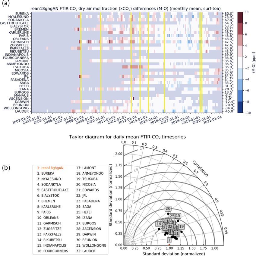
3832                  A. Agustí-Panareda et al.: Technical note: The CAMS greenhouse gas reanalysis from 2003 to 2020

      to initialise the following forecast over the subsequent      tivity peaking near the surface. The ground pixel size is
      12-hourly cycle.                                              typically between 30 and 60 km, and the swath width
                                                                    is about 960 km. There are no across-track gaps be-
Details of these four different components of the reanalysis        tween the ground pixels, but there are gaps in the along-
processing chain, as well as the approach followed to monitor       track direction as SCIAMACHY operates only part of
the assimilation of CO2 and CH4 satellite data, are provided        the time (approx. 50 %) in nadir observation mode. The
in the subsections below.                                           CO2 and CH4 column products are retrieved by the Uni-
                                                                    versity of Bremen (Reuter et al., 2011) and the Nether-
2.2    Satellite GHG observations                                   lands Institute for Space Research (SRON) (Franken-
The satellite measurements of radiances (L1 data) are pro-          berg et al., 2011), respectively. Both of the L2 prod-
cessed by satellite retrievals developed by various data            ucts are delivered by the ESA GHG-Climate Change
providers to derive information on the total and partial at-        Initiative (CCI; Buchwitz et al., 2015) and the C3S Cli-
mospheric column of CO2 and CH4 dry mole fraction (L2               mate Data Store (https://cds.climate.copernicus.eu, last
data). In the CAMS GHG reanalysis, only L2 products were            access: 18 March 2023).
used for CO2 and CH4 . With nadir-looking satellite instru-
ment geometries the L2 data provide vertically integrated         – TANSO-FTS – GOSAT. The Thermal And Near infrared
content with vertical sensitivity functions called either aver-     Sensor for carbon Observations – Fourier Transform
aging kernels (when an optimal estimation approach is used;         Spectrometer (TANSO-FTS) instrument on board the
Rodgers, 2000) or weighting functions, which provide infor-         Greenhouse Gases Observing Satellite (GOSAT) was
mation on where the retrieval sensitivity is located along the      developed by the Japan Aerospace Exploration Agency
vertical. The satellite products assimilated in this reanalysis     (JAXA) and launched in January 2009. TANSO-FTS
are all provided with an averaging kernel and prior informa-        measures radiances in the short-wave infrared band
tion or weighting functions (Massart et al., 2014, 2016). The       that provide information of total column CO2 and CH4
rationale for selecting the CO2 and CH4 satellite products is       mole fractions. Similar to SCIAMACHY, the sensitiv-
based on the availability of operational data in near real time     ity of the total column information provided by L2
as the strategy is to extend the CAMS GHG reanalysis to the         data peaks near the surface due to the spectral band
present by eventually running it at close to real time. Table 1     used. The ground pixel size is about 10 km, the swath
provides the specification for each of the assimilated satel-       is 750 km, and it has a revisit time of 3 d. In con-
lite CO2 and CH4 products, selected as the state-of-the-art         trast to SCIAMACHY, the GOSAT scan pattern con-
retrievals at the beginning of 2017, when the CAMS GHG              sists of non-consecutive individual ground pixels; i.e.
reanalysis production started. All of the L2 satellite products     it is not a gap-free scan pattern. For a general overview
are freely available from the Copernicus Climate Change             about GOSAT, see http://www.gosat.nies.go.jp/en/ (last
Service (C3S) Copernicus Climate Data Store (Alos et                access: 18 March 2023). The L2 retrieval product is en-
al., 2019; https://cds.climate.copernicus.eu/cdsapp#!/dataset/      gineered by the SRON (Schepers et al., 2012, 2016) and
satellite-carbon-dioxide, last access: 18 March 2023, for           delivered by the ESA GHG-CCI and the C3S Climate
CO2 and https://cds.climate.copernicus.eu/cdsapp#!/dataset/         Data Store (https://cds.climate.copernicus.eu).
satellite-methane, last access: 18 March 2023, for CH4 ). The
GHG reanalysis integrates the L2 GHG data from the follow-        – IASI – Metop A and B. The Infrared Atmospheric
ing satellite instruments.                                          Sounding Interferometer (IASI) instruments are on
                                                                    board the Meteorological Operational satellites Metop-
  – SCIAMACHY – Envisat. The SCanning Imaging Ab-                   A and Metop-B, launched in October 2006 and Septem-
    sorption spectroMeter for Atmospheric CartograpHY               ber 2012, respectively. The French National Centre
    (SCIAMACHY) instrument on board the Envisat satel-              for Space Studies (CNES) led the design and devel-
    lite was launched by the European Space Agency (ESA)            opment of the instruments in collaboration with the
    in March 2002, and it was developed by a consortium             European Organisation for the Exploitation of Mete-
    involving the Netherlands Space Office, the German              orological Satellites (EUMETSAT). The IASI instru-
    Aerospace Center and the Belgian Federal Science Pol-           ments measure the thermal infrared band with high
    icy Office. It measures radiance variations from the ul-        spectral resolution, enabling them to detect a wide
    traviolet to the near-visible infrared. The GHG L2 prod-        range of trace gas variations in the atmosphere, in-
    ucts use the nadir spectra of reflected and scattered solar     cluding CO2 and CH4 sensitive in the middle- and
    radiation in the near-infrared region. Satellite radiance       upper-tropospheric regions between 5 and 12 km al-
    observations in the near-infrared spectral region with          titude. IASI is an across-track-scanning system with
    the nadir-looking geometry are sensitive to changes in          a swath width of 2200 km providing global coverage
    CO2 and CH4 down to the Earth’s surface. The mea-               twice a day. The field of view is sampled by 2 × 2 pix-
    surements provide total column information with sensi-          els whose ground resolution is 12 km at nadir. Both

Atmos. Chem. Phys., 23, 3829–3859, 2023                                         https://doi.org/10.5194/acp-23-3829-2023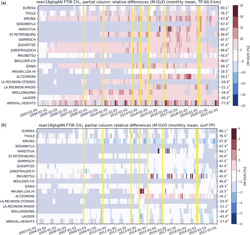
A. Agustí-Panareda et al.: Technical note: The CAMS greenhouse gas reanalysis from 2003 to 2020                                        3833

Figure 2. Schematic of the reanalysis cycling procedure. The flow diagram shows the steps and elements combined in the reanalysis. Surface
fluxes are used as boundary condition for the atmospheric forecasts. Satellite data are combined with the forecast using data assimilation to
produce an analysis (corrected 4D fields) to initialise the next forecast.

      CO2 and CH4 are engineered and delivered by the Cen-               in the analysis when the observing system coverage is sparse
      tre National de Recherche Scientifique (CNRS) Labora-              in space and time or when the observation error is large, and
      toire de Météorologie Dynamique (LMD) (Crevoisier et               the analysis is strongly influenced by the model forecast.
      al., 2009a, b, 2014). The two L2 products are delivered               Table 2 lists the datasets used to produce the CAMS re-
      by the ESA GHG-Climate Change Initiative (Buchwitz                 analysis, and Fig. 3 shows the seasonal cycle and trend of the
      et al., 2015) and the C3S Climate Data Store (https:               global mean values of each type of surface flux used in the
      //cds.climate.copernicus.eu).                                      simulations. They include the following datasets.

                                                                            – The first dataset includes fire emissions derived using
2.3   Surface fluxes and prescribed sources and sinks                         the CAMS Global Fire Assimilation System (GFAS)
                                                                              version 1.2 that assimilate fire radiative power observa-
The emissions and surface fluxes provide the surface bound-                   tions from satellite-based sensors (Kaiser et al., 2012).
ary conditions for the atmospheric concentrations of CO2 and                  GFAS produces daily estimates of wildfire and biomass
CH4 . They play a crucial role in determining the variability                 burning emissions. The emissions are injected at the
and growth rate of both greenhouse gases in the atmosphere.                   surface and distributed over the boundary layer by the
Errors in the budget of the total flux will result in system-                 model’s convection and vertical diffusion scheme.
atic errors or biases in the forecast of atmospheric CO2 and
CH4 . In the CAMS reanalysis, the surface fluxes (including                 – The second dataset includes anthropogenic emis-
sources and sinks) are not optimised by the assimilation sys-                 sions from the Emission Database for Global Atmo-
tem. This lack of surface flux optimisation can lead to biases                spheric Research (EDGAR) version 4.2FT2010 in-

https://doi.org/10.5194/acp-23-3829-2023                                                  Atmos. Chem. Phys., 23, 3829–3859, 2023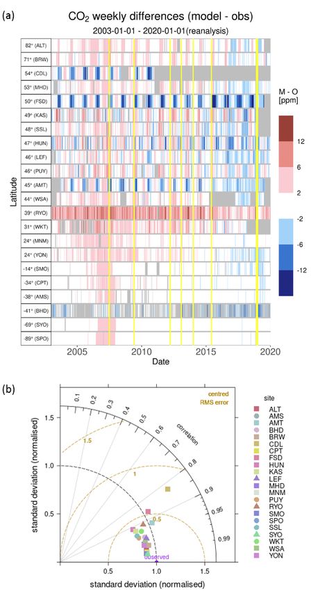
3834                     A. Agustí-Panareda et al.: Technical note: The CAMS greenhouse gas reanalysis from 2003 to 2020

Table 1. Specifications of the satellite data used in the CAMS GHG reanalysis.

  Gas     Instrument –      Period assimilated    Version (data provider)                       Reference             Peaking
          satellite         (yyyymmdd)                                                                                sensitivity
  CO2     SCIAMACHY         20030101–20120324     CO2_SCI_BESD (v02.01.02, IUP-UB)              Reuter et al.         Near surface
          – Envisat                                                                             (2011)
          IASI –            20070701–20150531     CO2_IAS_NLIS (v8.0, CNRS-LMD)                 Crevoisier et al.     Middle and upper
          Metop-A                                                                               (2009a)               troposphere
          IASI –            20130201–20181130     CO2_IAS_NLIS (v4.2_nrt, CNRS-LMD)                                   Middle and upper
          Metop-B           20181201–20201231     CO2_IAS_NLIS (v4.0_nrt, CNRS-LMD)                                   troposphere
          TANSO-FTS         20090601–20131231     CO2_GOS_SRFP (V2.3.6, SRON)                   Butz et al. (2011),   Near surface
          – GOSAT           20140101–20181231     CO2_GOS_SRFP (V2.3.8, SRON)                   Guerlet et al.
                            20190101–20201231     CO2_GOS_BESD (CAMS_NRT, IUP-UB)               (2013), Heymann
                                                                                                et al. (2015)
  CH4     SCIAMACHY         20030108–20100601     CH4_SCI_IMAP (v7.2, SRON)                     Frankenberg et al.    Near surface
          – Envisat                                                                             (2011)
          IASI –            20070701–20150630     CH4_IAS_NLIS (V8.3, CNRS-LMD)                 Crevoisier et al.     Middle and upper
          Metop-A                                                                               (2009b, 2014)         troposphere
          IASI –            20130201–20181130     CH4_IAS_NLIS (V8.1_nrt, CNRS-LDM)                                   Middle and upper
          Metop-B           20181201–20201231     CH4_IAS_NLIS (v4.0_nrt, CNRS-LDM)                                   troposphere
          TANSO-FTS         20090601–20131231     CH4_GOS_SRFP (V2.3.6, SRON)                   Butz et al. (2010),   Near surface
          – GOSAT           20140101–20181231     CH4_GOS_SRFP (V2.3.8, SRON)                   Schepers et al.
                            20190101–20201231     CH4_GOS_SRPR (CAMS_NRT, SRON)                 (2012)

Table 2. Specifications of the emission and surface fluxes used in the CAMS GHG reanalysis.

         Gas     Emission or flux type            Data provider – version
         CO2     CO2 and CH4 fire emissions       GFAS Version 1.2 (Kaiser et al., 2012)
                 CO2 ocean fluxes                 Takahashi climatology (Takahashi et al., 2009)
                 CO2 emissions from aviation      based on ACCMIP NO emissions from aviation scaled to annual total CO2
                                                  from EDGAR aviation emissions (Olivier and Janssens-Maenhout, 2012)
                 CO2 ecosystem fluxes bias        based on CHTESSEL (modelled online in IFS) (Boussetta et al., 2013; Agustí-
                 corrected with BFAS              Panareda et al., 2016)
                 CO2 anthropogenic emissions      EDGARv4.2FT2010 (2003–2010) (Olivier and Janssens-Maenhout, 2012)
         CH4     CH4 total natural emissions      based on EDGARv4.2FT2010 (2003–2010) (Olivier and Janssens-Maenhout,
                                                  2012), LPJ-WHyMe wetland climatology (Spahni et al., 2011), and other natu-
                                                  ral sources and sinks (Matthews et al., 1991; Ridgwell et al., 1999; Houweling
                                                  et al., 1999; Lambert and Schmidt, 1993; Sanderson, 1996)
                 CH4 chemical sink                monthly mean climatology of CH4 loss rate from Bergamaschi et al. (2009)
                 CH4 anthropogenic emissions      EDGARv4.2FT2010 (2003–2010) (Olivier and Janssens-Maenhout, 2012)

     ventory (Janssens-Maenhout et al., 2011; Olivier and                   ison Project (ACCMIP, Lamarque et al., 2013) nitric
     Janssens-Maenhout, 2012) excluding the short carbon                    oxide (NO) emissions scaled to the annual CO2 total
     cycle. The anthropogenic emissions are based on an-                    emissions from aviation from EDGAR. EDGAR pro-
     nual average values and include emissions from fossil                  duces global anthropogenic emissions for both CO2 and
     fuel combustion and leakage, agriculture, landfill and                 CH4 at a relatively high resolution of 0.1◦ (compared to
     waste, and aviation, the latter being based on the At-                 80 km resolution of the CAMS reanalysis). The prob-
     mospheric Chemistry and Climate Model Intercompar-                     lem with EDGAR is that the latest version available at

Atmos. Chem. Phys., 23, 3829–3859, 2023                                                    https://doi.org/10.5194/acp-23-3829-2023
A. Agustí-Panareda et al.: Technical note: The CAMS greenhouse gas reanalysis from 2003 to 2020 3835
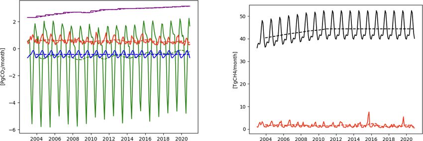
Figure 3. Monthly CO2 and CH4 surface fluxes. The CO2 fluxes (Pg CO2 per month) include modelled net ecosystem exchange (NEE)
fluxes (in green), anthropogenic emissions (in purple), ocean fluxes (in blue) and biomass burning emissions (in red). The total CH4 fluxes
(Tg CH4 per month) excluding biomass burning emissions are shown by the black line, and CH4 biomass burning emissions (Tg CH4 per
month) are depicted with the red line. The dashed lines show the 1-year running mean for each of the fluxes.
the time when the CAMS reanalysis started does not ex- – The fifth dataset includes a monthly modulation for CH4
tend beyond 2010. Anthropogenic emissions of CO2 are rice emissions that is implemented based on the sea-
extrapolated from 2010 to 2014 with the time series of sonal cycle of Matthews et al. (1991).
country totals from EDGARv4.3 (Janssens-Maenhout
et al., 2016), and from 2015 to 2020 a persistent growth – The sixth dataset includes a CH4 chemical sink that
based on the last available year (2014) is applied. CH4 is represented by a monthly mean climatological loss
anthropogenic emissions are fixed with the last year of rate from Bergamaschi et al. (2009) based on OH fields
available gridded data (2010) from 2011 to 2020. Note optimised with methyl chloroform (Bergamaschi et al.,
that CO2 and CH4 emissions are not adjusted for the 2005; Houweling et al., 1998) and stratospheric radicals
COVID-related emission reduction in 2020 (Le Quéré from the 2D photochemical Max Planck Institute (MPI)
et al., 2020). model (Brühl and Crutzen, 1993).
– The third dataset includes biogenic CO2 fluxes that are – Finally, the remaining datasets include a CH4 monthly
based on the online CHTESSEL module (Boussetta et soil sink (Ridgwell et al., 1999), CO2 and CH4 annual
al., 2013), which relates CO2 biogenic fluxes with radia- mean oceanic fluxes (Houweling et al., 1999; Lambert
tion, precipitation, temperature, humidity and soil mois- and Schmidt, 1993; Takahashi et al., 2009), and CH4
ture. CHTESSEL is used in conjunction with the bio- monthly mean fluxes from termites (Sanderson, 1996)
genic flux adjustment system (BFAS), which improves and wild animals (Houweling et al., 1999).
the continental budget of CO2 fluxes by combining in-
formation from flux estimates of a global flux inver- 2.4 Forecast model
sion system (Chevallier et al., 2010), land use infor-
mation and CHTESSEL online fluxes (Agustí-Panareda The CAMS GHG reanalysis has been produced using the
et al., 2016). The two-way interaction between the at- IFS model. The same model is used to produce operational
mospheric forecast and the surface fluxes depicts how NWPs at ECMWF, and the CAMS global forecast and anal-
the forecast influences the surface fluxes and vice versa yses are used for reactive gas, aerosols and greenhouse gases
via the coupling of the biogenic fluxes to the atmo- at ECMWF (Fleming et al., 2015; Agustí-Panareda et al.,
spheric forecast (radiation, temperature, humidity and 2017, 2022). The IFS model version used is IFS CY42R1,
soil moisture) and the influence of the resulting biogenic the same as in the CAMS reanalysis for reactive gases and
fluxes on the atmospheric CO2 forecast. aerosols (Inness et al., 2019). The forecasting model uses
a reduced Gaussian grid with a resolution of TL255, corre-
– The fourth dataset includes wetland CH4 monthly mean sponding to a horizontal resolution of approximately 80 km
emissions that come from a climatology (1990–2008) and 60 hybrid sigma–pressure vertical levels from the sur-
based on the LPJ-WHyMe model, which is constrained face to 0.1 hPa. The tracer advection is computed using
by SCIAMACHY observations (Spanhi et al., 2011). a non-mass-conserving, semi-implicit and semi-Lagrangian
scheme (Temperton et al., 2001; Diamantakis and Magnus-
https://doi.org/10.5194/acp-23-3829-2023 Atmos. Chem. Phys., 23, 3829–3859, 2023
3836                 A. Agustí-Panareda et al.: Technical note: The CAMS greenhouse gas reanalysis from 2003 to 2020

son, 2016). This scheme leads to an error growth that can        serve to initialise the next forecast at the full TL255 reso-
dominate the signal in the model simulations if it is not cor-   lution.
rected. Thus, a mass fixer is required to ensure mass conser-       The background errors for CO2 and CH4 were produced
vation at every time step (Diamantakis and Agustí-Panareda,      from an ensemble of data assimilations (Massart et al., 2016),
2017). The mass fixer is particularly important for long-lived   which allows the calculation of differences between pairs of
greenhouse gases for which the interesting signals to mon-       background fields that have the characteristics of the back-
itor, e.g. trends or annual growth rates and large-scale spa-    ground errors. The background errors for the greenhouse gas
tial gradients, are weak compared to the large background        species are univariate, which means that there is no correla-
values. The transport model also includes a turbulent mix-       tion between the greenhouse gas species and the dynamical
ing scheme (Sandu et al., 2013) and a convection scheme          fields. Hence, each species is assimilated independently of
(Bechtold et al., 2014). For the CH4 chemical sink in the tro-   the others. The background errors used for both the green-
posphere and the stratosphere, climatological loss rates de-     house gas species and the dynamical fields are also constant
rived from the Max Planck Institute photochemical model are      in time. In the ECMWF data assimilation system, the back-
used (Bergamaschi et al., 2009). Full documentation of the       ground error covariance matrix is given in a wavelet formula-
IFS can be found at https://www.ecmwf.int/en/publications/       tion (Fisher, 2004, 2006). This allows both spatial and spec-
ifs-documentation (last access: 18 March 2023).                  tral variations of the horizontal and vertical background error
                                                                 covariances globally. Figure 4 shows the global mean of the
2.5    Analysis procedure (data assimilation)                    standard deviation and average horizontal correlation length
                                                                 scales for both CH4 and CO2 . Following experimentation,
The IFS system uses an incremental formulation of the            the correlation length scales between the background errors
four-dimensional variational technique (4D-Var). The 4D-         were manually reduced in the atmospheric boundary layer
Var technique consists of minimising a cost function that        (1 km from the surface).
combines the model information and the observation infor-
mation in order to obtain the best possible state of the atmo-
                                                                 2.6   Monitoring the data assimilation system
sphere (analysis) accounting for the model and observation
errors. The incremental 4D-Var cost function is quadratic and    The time series of the departures (or differences) between
is formulated as follows:                                        the analysis (AN) and the assimilated satellite data (hereafter
        1                                                        referred to as observations, OBS), as well as those between
J (δx) = (δx − δxb )T B−1 (δx − δxb )                            the underlying model simulation (or background, BG) and
        2                                                        the OBS, are used to monitor the performance of the analy-
        1
       + (Gδx − d) R−1 (Gδx − d) ,                         (1)   sis system and are shown in Fig. 5 (for CO2 ) and Fig. 6 (for
        2                                                        CH4 ). For each satellite retrieval product, both the BG depar-
where δx is the increment, i.e. the difference between the       tures (OBS–BG, green lines) and the AN departures (OBS–
model state x and the first guess xg , δxb is the difference     AN, red lines) are plotted (Figs. 5a and 6a: SCIAMACHY;
between the background (the forecast started from the pre-       Figs. 5b and 6b: IASI-A; Figs. 5c and 6c: IASI-B; Figs. 5d
vious analysis) and the first guess, B is the background error   and 6d: GOSAT), together with the number of observations
covariance matrix, R is the observation error covariance ma-     assimilated monthly (blue lines). Overall, both the random
trix, and G is the observation operator or forward operator      (i.e. standard deviation, dashed lines) and systematic compo-
that translates the information from model space to observa-     nents of the departures (i.e. average values, solid lines) are
tion space. The innovation vector is d = y − Gxg , where y       shown to be reduced by the assimilation process, as high-
is the observation vector and xg is the first guess. When the    lighted by the AN departures (red lines) being closer to zero
minimisation of the cost function is complete, δx is added to    than the BG departures (green lines). Note that the difference
xg to provide the analysis.                                      between the BG and the AN departure is equal to the anal-
                                                                 ysis increments associated with the related observations (i.e.
xa = xg + δx                                               (2)   AN–BG).
                                                                    The number of observations assimilated is different for
The analysis is performed over 12 h assimilation windows         each satellite instrument and varies with time. IASI generates
from 09:00 to 21:00 and from 21:00 to 09:00 UTC. The in-         the largest number of data, with both instruments (IASI-A
cremental 4D-Var assimilation involves the stepwise minimi-      and IASI-B) providing between 150 000 and 200 000 XCO2
sation of the linearised cost function (Eq. 1) by updating the   or XCH4 data per month. The observations taken by SCIA-
first guess xg and increasing the resolution. In the CAMS        MACHY oscillate between 25 000 and 50 000 data per month
reanalysis setup, two minimisations are completed succes-        for CH4 and between 5000 and 10 000 data per month for
sively at TL95 (approximately 210 km) and TL159 (approxi-        CO2 . The number of GOSAT XCO2 data fluctuates around
mately 110 km) spectral truncations. Once the assimilation       2500, whereas GOSAT XCH4 measurements are comprised
procedure is completed, an analysis is generated that will       of between 5000 and 10 000 data per month. It is also clear

Atmos. Chem. Phys., 23, 3829–3859, 2023                                           https://doi.org/10.5194/acp-23-3829-2023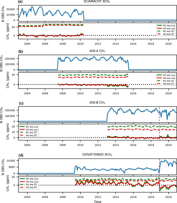
A. Agustí-Panareda et al.: Technical note: The CAMS greenhouse gas reanalysis from 2003 to 2020                                      3837

Figure 4. Model background error for CO2 and CH4 used in the CAMS GHG reanalysis: (a, b) global mean standard deviation and
(c, d) global mean error correlation length scale across the vertical levels.

from Figs. 5a, d and 6a, d that fewer XCO2 and XCH4 data                    increasing atmospheric CO2 . Note that this has been cor-
from SCIAMACHY, IASI and GOSAT-TANSO are assimi-                            rected with v9.1 (available on the C3S data store). A sudden
lated during the winter months. A vertical dashed magenta                   change in the IASI-B XCO2 departures is visible in Fig. 5c
line in Figs. 5c, d and 6c, d indicates when the near-real-time             around December 2018, corresponding to the switch from
satellite products started to be assimilated in early 2019. This            the ESA-CCI reprocessed dataset to a near-real-time LMD
transition produced an abrupt change in the quality and avail-              dataset used operationally in the CAMS GHG analysis. The
ability of both IASI and GOSAT retrievals.                                  transition to a new dataset was made necessary as the re-
   The modelled XCO2 is systematically larger than the ob-                  analysis production was running close to real time and repro-
servations (leading to overall negative BG departures) be-                  cessed observations were not available. After the transition to
cause of the biases in the total fluxes (see Sect. 2.3). There-             near-real-time observations, the IASI XCO2 increments are
fore, all instruments produced negative departures until 2013               reduced to almost zero, as hinted to by the overlap between
(Fig. 5). From 2013 to 2019, the modelled values of XCO2                    the red (AN departure) and green lines (BG departure) in
became smaller than those measured by GOSAT (Fig. 5d),                      Fig. 5c. At the same time, a drop in the number of assimilated
while the model continued to (slightly) overestimate the IASI               IASI XCO2 observations is observed (blue line, Fig. 5c). To-
XCO2 observations in the middle to upper troposphere. This                  gether with a drastic reduction in the magnitude of the in-
overestimation is consistent with a drift in the IASI CO2 data              crements, a large negative bias of approximately 5 ppm in
towards a growing negative bias. After 2018, part of the drift              both the AN and BG departures emerges. This degradation
is due to the fact that IASI (version v4.0) is saturated with               in the quality of the IASI-B XCO2 observations in the near-

https://doi.org/10.5194/acp-23-3829-2023                                                   Atmos. Chem. Phys., 23, 3829–3859, 2023
3838                   A. Agustí-Panareda et al.: Technical note: The CAMS greenhouse gas reanalysis from 2003 to 2020

Figure 5. Time series of the global monthly number of XCO2 satellite data (blue) and monthly mean CO2 analysis (AN) and model
background (BG) departures of the various observations (OBS) assimilated in the reanalysis (AN–OBS and BG–OBS in red and green,
respectively; see the legend). The solid lines show the monthly average of the departures, and the dashed lines show the monthly standard
deviations. The dashed magenta line indicates the switch to the near-real-time satellite products. Note that the range of values on the y axis
varies depending on the satellite product.

real-time dataset is due to the change in the correction of              uct (Heymann et al., 2015; Massart et al., 2016), as shown
the non-linearity of the detector of IASI-B that was made by             in Fig. 5d. Consequently, the standard deviation of both the
CNES and EUMETSAT on 17 August 2018 that introduced                      AN and the BG departures increases (dashed lines, Fig. 5d),
a bias of ∼ 0.2 K into the channels used to perform the CO2              suggesting that the near-real-time data are noisier than the
retrieval. This change has been corrected in the versions of             reprocessed dataset from ESA-CCI.
IASI-B MT-CO2 that are available on the C3S data store, but                 The mean XCH4 departures (both AN and BG) of SCIA-
these versions were not used for this reanalysis. In January             MACHY and IASI are relatively small (a few ppb) compared
2019, there was also a transition from the ESA-CCI GOSAT                 to GOSAT (up to 10 ppb) throughout the entire time period
XCO2 retrievals to the near-real-time IUP-UB retrieval prod-             (see the solid red and green lines in Fig. 6). The XCH4 SCIA-

Atmos. Chem. Phys., 23, 3829–3859, 2023                                                     https://doi.org/10.5194/acp-23-3829-2023
A. Agustí-Panareda et al.: Technical note: The CAMS greenhouse gas reanalysis from 2003 to 2020                                          3839

Figure 6. Time series of the global monthly number of XCH4 satellite data (blue) and monthly mean CH4 analysis (AN) and model
background (BG) departures of the various observations (OBS) assimilated in the reanalysis (AN–OBS and BG–OBS in red and green,
respectively; see the legend) for different satellite products. The solid lines show the monthly average of the departures, and the dashed lines
show the monthly standard deviations. The dashed magenta line indicates the switch to the near-real-time satellite products. Note that the
range of values on the y axis varies depending on the satellite product.

MACHY data were not used from 9 April 2012 onwards                        (see the dashed magenta line in Fig. 6d). Both the AN and
(Fig. 6a). The standard deviation of both the AN and BG de-               the BG departures change sign, indicating that while up to
partures are smaller for GOSAT (around 10 ppb, dashed lines               2019 both the analysis and model were underestimating the
in Fig. 6d) than for SCIAMACHY (around 20 ppb, dashed                     GOSAT observations, they started to overestimate them af-
lines in Fig.6a), indicating that GOSAT provides less noisy               ter 2019. Since there was no modification to the model used
observations. Similar to what was observed for CO2 , a dis-               for the reanalysis over this period, the cause of this negative
continuity in the mean AN and BG departures of GOSAT                      bias emerging in both the AN and the BG departures since
XCH4 emerges in January 2019, corresponding to transition                 2019 can only be attributed to the NRT GOSAT XCH4 ob-
from the ESA-CCI dataset and the NRT SRON retrievals                      servations, and in particular to the fact that they are generated

https://doi.org/10.5194/acp-23-3829-2023                                                    Atmos. Chem. Phys., 23, 3829–3859, 2023
3840                   A. Agustí-Panareda et al.: Technical note: The CAMS greenhouse gas reanalysis from 2003 to 2020

                                                                     (Fig. 8), there is a large variability in the CO2 error between
                                                                     continental stations influenced by local fluxes (e.g. CDL,
                                                                     FSD, AMT, HUN; see Table A1) and oceanic stations sam-
                                                                     pling well-mixed air (e.g. ALT, BRW, MHD). Continental
                                                                     stations show large error variations with season (e.g. CDL,
                                                                     HUN) and show an underestimation of CO2 in the summer
                                                                     and an overestimation in the winter, indicating an underesti-
                                                                     mation of the amplitude of the CO2 seasonal cycle largely
                                                                     driven by vegetation growth. Differences between stations
                                                                     will be determined by the footprint of observations having
Figure 7. Map with observation sites used in the evaluation of       different contributions of fluxes from different biomes and
the CAMS GHG reanalysis: the marine boundary layer (MBL,             from anthropogenic emissions. The accuracy of such fluxes
blue squares) includes NOAA MBL reference sites used to com-         can vary geographically.
pute the NOAA global mean CO2 and CH4 mole fraction product             Overall, there is positive bias of a few parts per million
(see https://gml.noaa.gov/ccgg/mbl/mbl.html, last access: 18 March   between 2003 and 2015 in the baseline surface stations (e.g.
2023, for further details), SFC (black circles) corresponds to the   BRW, SMO, SPO), which is consistent with the XCO2 er-
in situ near-surface continuous observations of CO2 and CH4 , TC-
                                                                     ror at the TCCON sites (Fig. 9). This positive bias decreases
CON and NDACC sites are depicted by red and orange triangles,
                                                                     from 2007 to 2015 when IASI-A CO2 data are assimilated,
and AirCore sites are shown by cyan circles.
                                                                     with values lower than 2 ppm, and becomes negative from
                                                                     2015 to 2019 (from 0 to −2 ppm). From 2019 onwards,
by using an extrapolated XCO2 value in the proxy retrieval.          there is a positive trend in the bias, and it becomes positive
In addition, the number of assimilated NRT GOSAT XCH4                (> +2 ppm) in 2020. There is consistency between the col-
observations approximately doubles (blue line in Fig. 6d).           umn and surface biases, with a general positive bias at back-
Note that the switch to the near-real-time retrievals for IASI-      ground stations before 2015 and a negative bias after 2015
B XCH4 has a much more marginal impact on the system                 (up to 2019) at the surface stations, although there are no
(Fig. 6c).                                                           data in 2020 from the surface stations.
                                                                        The synoptic and large-scale variability of CO2 is well rep-
                                                                     resented by the reanalysis (Fig. 9b). The root-mean-square
3     Evaluation with independent observations                       error at TCCON stations is below 0.8 ppm for XCO2 . The
                                                                     normalised standard deviation is around 1.0 (±0.3), and the
Validation against a set of independent observations has been
                                                                     Pearson correlation coefficient is larger than 0.8.
performed on the 18 years of the CAMS GHG reanalysis
span. The independent data include different types of obser-
vations (see Fig. 7): in situ near-surface continuous observa-       3.1.2   Methane
tions of CO2 and CH4 mole fractions from the collaborative
                                                                     The CH4 reanalysis fields are generally in good agreement
ObsPack datasets (Masarie et al., 2014; Schuldt et al., 2020,
                                                                     with surface and tropospheric column observations, with typ-
2021; NOAA Carbon Cycle Group ObsPack Team, 2019; see
                                                                     ical weekly and monthly errors within ±40 and ±25 ppb,
Table A1), dry-air column-averaged mole fractions from the
                                                                     respectively (Figs. 10, 11 and 12). Stratospheric partial
Total Carbon Column Observing Network (TCCON; Wunch
                                                                     columns compared to the NDACC data reveal a positive bias
et al., 2011, 2015), tropospheric and stratospheric partial
                                                                     that is of the same order as the reported measurement un-
columns for CH4 from the Network for the Detection of At-
                                                                     certainty of 7 % (Fig. 10a). The averaged relative differences
mospheric Composition Change (NDACC; De Mazière et
                                                                     in the troposphere across all NDACC sites are −0.4 % for
al., 2018) (see Table A2), AirCore vertical profiles of CO2
                                                                     the reanalysis (Fig. 11b), which is well within the measure-
and CH4 mole fractions (Karion et al., 2010; Baier et al.,
                                                                     ment’s uncertainty. The reanalysis overestimates the column-
2021), and the NOAA global mean CO2 and CH4 mole frac-
                                                                     averaged CH4 compared to TCCON observations (Fig. 12)
tion product based on the Greenhouse Gas Marine Boundary
                                                                     for most mid- and high-latitude sites, with a relative differ-
Layer Reference (Conway et al., 1994; Dlugokencky et al.,
                                                                     ence of up to 2.5 %, but shows a good agreement for the low-
1994; Masarie and Tans, 1995).
                                                                     latitude sites at Izaña, Darwin and Wollongong. At the sur-
                                                                     face the bias is overall positive up to 2007 (Fig. 10). With the
3.1     Surface and column data                                      introduction of IASI, the biases are reduced. However, with
                                                                     the switch to near-real-time satellite data, the bias become
3.1.1    Carbon dioxide
                                                                     negative at all sites, reaching values lower than −20 ppb.
Overall, the error is within ±10 and ±4 ppm for most of                 Differences between the surface and total column biases
the near-surface and total column stations, respectively, for        stem from the fact that the model suffers from large posi-
the whole 18-year period (Figs. 8 and 9). Near the surface           tive biases above the tropopause (between 100 and 10 hPa)

Atmos. Chem. Phys., 23, 3829–3859, 2023                                               https://doi.org/10.5194/acp-23-3829-2023
A. Agustí-Panareda et al.: Technical note: The CAMS greenhouse gas reanalysis from 2003 to 2020 3841 Figure 8. (a) Mosaic plot of CO2 weekly biases (in ppm) of the CAMS GHG reanalysis compared to surface continuous observations of CO2 mole fraction obtained from the GLOBALVIEWplus CO2 ObsPack v6.0 (Schuldt et al., 2020) listed in Table A1. Each coloured vertical line represents a weekly mean. Vertical yellow lines depict the changes in the assimilated data documented in Figs. 1, 5 and 6. Grey shading indicates no observations are available. (b) Taylor diagrams for the site-dependent CO2 comparison of the CAMS GHG reanalysis against the same observations used in (a). The standard deviation is normalised by dividing the observed and modelled time series by the standard deviation of the observations. The model has higher (lower) variability compared to the observed data if the site is plotted with a distance larger (smaller) than 1 from the origin. https://doi.org/10.5194/acp-23-3829-2023 Atmos. Chem. Phys., 23, 3829–3859, 2023
3842                   A. Agustí-Panareda et al.: Technical note: The CAMS greenhouse gas reanalysis from 2003 to 2020

Figure 9. (a) Mosaic plot of the CAMS GHG reanalysis biases at all TCCON sites (see Table A2) for the column-averaged dry mole
fraction of CO2 (ppm) (XCO2 ) averaged daily around local noon (±2.5 h). Vertical yellow lines depict the changes in the assimilated data
documented in Figs. 1, 5 and 6. Grey shading indicates no observations are available. (b) Taylor diagrams for the station-dependent XCO2
comparison of the CAMS GHG reanalysis against TCCON Fourier transform infrared (FTIR) data. The standard deviation is normalised by
dividing the observed and modelled time series by the standard deviation of the model time series. The model has higher (lower) variability
compared to the observed data if the site is plotted with a distance smaller (larger) than 1 from the origin.

of about 80–100 ppb during the months between September                 underestimation is also seen in the TCCON time series. In
and November (Figs. 5d and 6d of Verma et al., 2017) that               spring and summer there is an overestimation of CH4 near the
affect the total column average. This stratospheric bias can-           surface and in the total column. These biases are related to
not be corrected systematically by CH4 satellite data from              errors in the seasonal cycle of surface emissions, most likely
SCIAMACHY, GOSAT and IASI.                                              from agriculture and wetlands, and the accuracy of the rep-
   For all observations (surface, partial and total columns)            resentation of the hydroxyl radical (OH) sink, which overall
CH4 shows a seasonality in the relative difference between              have larger values in the climatology compared to CAMS IFS
observations and the reanalysis. The magnitude of the dif-              (CB05-BASCOE) atmospheric chemistry model OH (Segers
ference is site dependent. During local autumn and win-                 et al., 2020b; Williams et al., 2022). The XCH4 root-mean-
ter months the relative bias is increased (underestimation)             square error is around 1.4 ppb, and the Pearson correlation
at most surface sites and in the tropospheric columns. This             coefficient is larger than 0.7 for XCH4 except for some out-

Atmos. Chem. Phys., 23, 3829–3859, 2023                                                   https://doi.org/10.5194/acp-23-3829-2023
A. Agustí-Panareda et al.: Technical note: The CAMS greenhouse gas reanalysis from 2003 to 2020                                       3843

Figure 10. (a) Mosaic plot of CH4 biases (in ppb) compared to surface continuous observations from GLOBALVIEWplus CH4 ObsPack v1.0
data product (Cooperative Global Atmospheric Data Integration Project, 2019) listed in Table A1. Each coloured vertical line represents a
weekly mean. Vertical yellow lines depict the changes in the assimilated data documented in Figs. 1, 5 and 6. Grey shading indicates no
observations are available. (b) Taylor diagrams for the site-dependent CH4 comparison of the CAMS GHG reanalysis against same as the
observations used in (a). The standard deviation is normalised by dividing the observed and modelled time series with the standard deviation
of the observations. The model has higher (lower) variability compared to the observed data if the site is plotted with a distance larger
(smaller) than 1 from the origin.

https://doi.org/10.5194/acp-23-3829-2023                                                 Atmos. Chem. Phys., 23, 3829–3859, 2023
3844                   A. Agustí-Panareda et al.: Technical note: The CAMS greenhouse gas reanalysis from 2003 to 2020

Figure 11. Mosaic plot of seasonal relative CH4 biases at all FTIR sites (see Table A2) for the stratospheric columns (a) and tropospheric
columns (b) from NDACC. Vertical yellow lines depict the changes in the assimilated data documented in Figs. 1, 5 and 6. Grey shading
indicates no observations are available.

liers (Fig. 12b), indicating a good representation of the syn-            Figure 13 shows that the largest mean errors occur (i) near
optic variability (as for XCO2 ).                                      the surface with a strong influence from surface fluxes,
                                                                       (ii) in the upper troposphere–lower stratosphere (UTLS) re-
3.2    Vertical profiles                                               gion (between 500 and 100 hPa) with a strong influence from
                                                                       long-range transport, (iii) in the stratosphere (above 100 hPa)
The uncertainty in the CAMS GHG reanalysis varies with                 where uncertainties associated with chemical loss of CH4
height, and the accuracy of the analysis vertical profiles de-         and the meteorology driving the tracer transport are largest,
pends mostly on the underlying model uncertainty, as the               and the fact that satellite data used here are not able to con-
satellite data assimilated in the reanalysis only provide in-          strain the stratospheric CO2 and CH4 in the reanalysis. Near
tegrated total or partial atmospheric columns. The reanalysis          the surface, there is a positive CO2 bias associated with an
has been evaluated using observations of CO2 and CH4 ver-              overestimation of the total flux in the model and a negative
tical profiles (Karion et al., 2010; Baier et al., 2021) from          CH4 bias that stems from both errors in the emissions and
the NOAA AirCore dataset v20210813. It includes 133 ver-               the chemical loss rate in the troposphere. The negative CO2
tical profiles from the surface to the lower stratosphere (up to       bias in the UTLS agrees with the tendency of the model to
around 40 hPa) from 2012 to 2020 at the seven sites listed in          underestimate fine-scale higher-valued CO2 streamers asso-
Table A3.                                                              ciated with long-range transport. The large positive CH4 bias

Atmos. Chem. Phys., 23, 3829–3859, 2023                                                   https://doi.org/10.5194/acp-23-3829-2023
A. Agustí-Panareda et al.: Technical note: The CAMS greenhouse gas reanalysis from 2003 to 2020 3845 Figure 12. (a) Mosaic plot of monthly biases at all TCCON sites for the column-averaged mole fractions XCH4 (ppb) averaged daily around local noon (±2.5 h). Vertical yellow lines depict the changes in the assimilated data documented in Figs. 1, 5 and 6. Grey shading indicates no observations are available. (b) Taylor diagrams for the station-dependent XCH4 comparison of the CAMS GHG reanalysis against TCCON FTIR data. The standard deviation is normalised by dividing the observed and modelled time series by the standard deviation of the model time series. The model has higher (lower) variability compared to the observed data if the site is plotted with a distance smaller (larger) than 1 from the origin. in the stratosphere of around 200 ppb is consistent with the atmospheric mole fractions, i.e. without adjusting the emis- positive biases with respect to NDACC stratospheric column sions in the data assimilation process, nor it is able to reduce (Fig. 11a) and the documented model biases with respect to the stratospheric errors in the model (Massart et al., 2017; MIPAS and ACE-FTS by Verma et al. (2017). The errors as- Verma et al., 2017). The vertical profiles have a large vari- sociated with the stratospheric chemical sink are thought to ability from day to day, as shown in Fig. 14 with a sequence be the largest contributor to the stratospheric CH4 bias, as of profiles at Traînou (France). The CAMS GHG reanalysis shown by tests using the IFS CB05-BASCOE chemical loss is able to capture these synoptic variations in the vertical pro- rate (not shown here). In general, the reanalysis underesti- file, consistent with its skill in representing XCO2 and XCH4 mates the CO2 vertical gradient across the tropopause. This synoptic variability (Figs. 9b and 12b). For a full catalogue underestimation leads to a positive bias for CO2 in the lower of all the individual AirCore vertical profiles used in Fig. 13, stratosphere of around 2 ppm. The analysis is not able to re- see the Supplement. move the large errors near the surface by only adjusting the https://doi.org/10.5194/acp-23-3829-2023 Atmos. Chem. Phys., 23, 3829–3859, 2023
3846                   A. Agustí-Panareda et al.: Technical note: The CAMS greenhouse gas reanalysis from 2003 to 2020

Figure 13. Vertical profiles of mean error (model minus observation, M–O) of CAMS CO2 (a) and CH4 (b) reanalysis with respect to
AirCore observations comprising 133 profiles at seven sites (listed in Table A3) over the period from 2012 and 2020. The blue shading shows
the ± standard deviation of M–O with respect to the mean error. The vertical dashed black line depicts the zero mean error.

Figure 14. Vertical mole fraction profiles of CO2 and CH4 from the CAMS GHG reanalysis (dashed line) and AirCore observations (solid
line) at Traînou (France; see Table A3) over the period in June 2019.

3.3    Trends                                                           Greenhouse Gas Reference Network (GGGRN) observations
                                                                        (https://gml.noaa.gov/ccgg/about.html, last access: 18 March
                                                                        2023; Andrews et al., 2014; Conway et al., 1994; Dlugo-
Although this reanalysis uses a consistent underlying model
                                                                        kencky et al., 1994) in Fig. 15. Changes in the assimilated
and reprocessed observations of CO2 and CH4 , the current
                                                                        satellite data have a clear impact on the evolution of the
system is not able to provide an accurate enough atmo-
                                                                        global annual mean values of CO2 and CH4 in the CAMS
spheric mole fraction for use in estimating trends and atmo-
                                                                        GHG reanalysis. The reanalysis has a positive global bias in
spheric growth rates as computed by the changes in global
                                                                        near-surface CO2 and CH4 of a few parts per million and
mean CO2 and CH4 from 1 year to the next. The CO2 and
                                                                        around 20 ppb, respectively, from 2003 to 2007. Note that
CH4 global annual means based on marine boundary layer
                                                                        this positive bias in the annual global mean does not imply
(MBL) reference sites are compared to the NOAA Global

Atmos. Chem. Phys., 23, 3829–3859, 2023                                                   https://doi.org/10.5194/acp-23-3829-2023
A. Agustí-Panareda et al.: Technical note: The CAMS greenhouse gas reanalysis from 2003 to 2020 3847
that the bias will be positive everywhere, as shown by the including its systematic errors (see the discussion of
negative surface CH4 biases at the AirCore sites (Fig. 13) stratospheric biases in Sect. 3.2).
and the large temporal and geographical variability in the
weekly bias illustrated in Figs. 8 and 10. After the intro- 3. Changes in satellite retrievals affect the quality of the
duction of IASI in 2007 the global bias decreases and is at observations used in the CAMS GHG reanalysis. For
its lowest during the period when the number of observa- example, the switch from the CCI reprocessed satel-
tions is largest in 2013 and 2014 (Figs. 5 and 6). Finally, lite products to the near-real-time products is associated
the change to the near-real-time satellite retrievals in 2019 with a marked change in the bias and random error (i.e.
and the incorrect trend in the emissions during the COVID- standard deviation) of the departures from XCO2 and
related slowdown period in 2020 (Le Quéré et al., 2020) lead XCH4 GOSAT observations and in the bias of the depar-
to changes in the global bias from negative to positive for tures from the XCO2 IASI-B observations. This large
CO2 and from positive to negative for CH4 . These changes increase in the bias of the assimilated CO2 and CH4
in the global bias are consistent with the changes in the errors observations from 2019 onwards results in a large in-
with respect to total column and near-surface observations in crease in the bias of the CAMS GHG reanalysis in 2019
Figs. 8 to 12. It is important to note that the changes in global and 2020, which has implications for the trend analysis
bias associated with changes in the assimilated data are of the (Sect. 3.3).
same order of magnitude as the observed atmospheric growth
4. The fixed climatological chemical loss rate of CH4
rates of CO2 (https://gml.noaa.gov/ccgg/trends, last access:
(Sect. 2.3) has been shown to overestimate the atmo-
18 March 2023) and CH4 (https://gml.noaa.gov/ccgg/trends_
spheric CH4 chemical sink by Segers et al. (2020b). Pre-
ch4, last access: 18 March 2023). For this reason, this reanal-
liminary tests coupling the IFS to the atmospheric loss
ysis product is not suitable for trend analysis.
rate derived from CB05-BASCOE chemistry have in-
deed shown a large reduction in the CH4 negative bias
4 Limitations and caveats at mid-latitudes. Systematic errors in the CH4 chemical
sink used in this reanalysis may have contributed further
This section provides an overview of the shortcomings of the to enhancing the large negative CH4 bias in the CAMS
CAMS GHG reanalysis that users should consider when in- GHG reanalysis over the last period in 2020, when the
terpreting the data. The main issues documented in the pre- increase in the CH4 growth rate is linked to a decrease
vious sections are summarised below. in chemical loss rate (Stevenson et al., 2022).
1. Emissions are prescribed and not adjusted by the data 5. The large CH4 and CO2 biases in the stratosphere are
assimilation system in the CAMS reanalysis (Sect. 2.3). currently under investigation. The CH4 stratospheric
This leads to a growing model error for CO2 and CH4 bias is mainly associated with the use of a climatologi-
that can be difficult to correct with a sparse observing cal loss rate (Sect. 2.3), as preliminary tests using a dif-
system and 12 h assimilation window. In addition, the ferent chemical loss rate based on IFS CB05-BASCOE
prescribed emissions are not available as near-real-time simulations show that the bias in CH4 is greatly re-
data, which means they are either kept fixed since the duced.
last year available (e.g. 2010 for CH4 ) or extrapolated
with a climatological trend as was done for CO2 (see 6. Changes in systematic errors with time due to model
details in Sect. 2.3). Because of this, the CAMS GHG error and changes in observation coverage and quality
reanalysis is not suitable to investigate the impact of will affect trend analysis (see Sect. 3.3).
local emission changes, such as COVID impact stud-
An up-to-date list of the known issues of the CAMS re-
ies, which require a large local emission adjustment to
analysis can be found on the online CAMS documen-
the prescribed inventories (e.g. Doumia et al., 2021) and
tation website (https://confluence.ecmwf.int/display/CKB/
atmospheric inversion systems to estimate the changes
CAMS%3A+Reanalysis+data+documentation, last access:
(e.g. McNorton et al., 2022).
18 March 2023). Some of these issues will also be addressed
2. Changes in satellite data used with different temporal, in the future CAMS reanalysis (planned to start production
horizontal and vertical coverage cause changes in the in 2024), including the improvement of the prescribed emis-
quality of the reanalysis. For example, winter seasons sion trends, the consistent use of satellite retrieval products
have a lower number of observations because of light and the use of a variable CH4 chemical loss rate.
conditions and the higher frequency of cloud presence.
This affects the quality of the seasonal cycle and the 5 Summary and conclusions
inter-hemispheric gradient. Similarly, in regions where
there is no observation coverage, such as the strato- This technical report documents the first CAMS IFS reanaly-
sphere, the reanalysis is based on the underlying model sis of CO2 and CH4 produced by ECMWF that complements
https://doi.org/10.5194/acp-23-3829-2023 Atmos. Chem. Phys., 23, 3829–3859, 2023You can also read