TOWARDS PRACTICAL SIGNAL-DEPENDENT NOISE MODELS IN PATH TRACING - Duong Trung Kien - Trepo
←
→
Page content transcription
If your browser does not render page correctly, please read the page content below
Duong Trung Kien

             TOWARDS PRACTICAL
SIGNAL-DEPENDENT NOISE MODELS IN
                   PATH TRACING

                                Bachelor’s thesis
                  Examiners: Prof. Alessandro Foi
                                       April 2020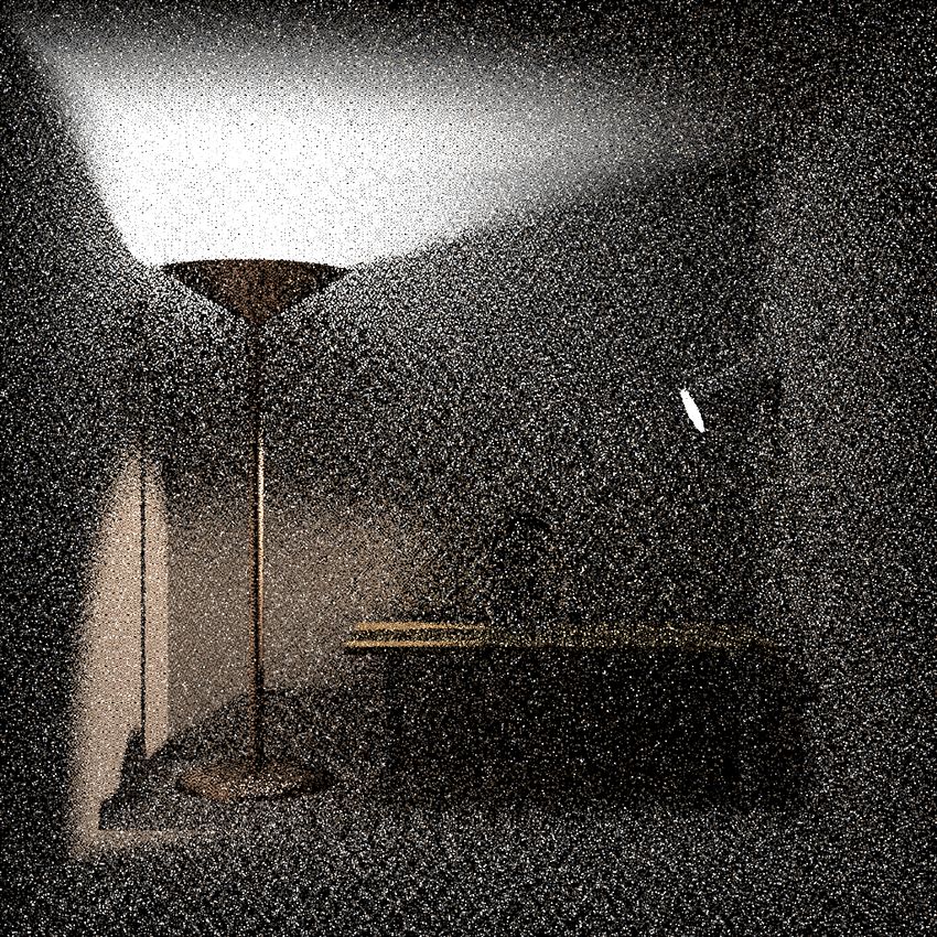
i

ABSTRACT
Duong Trung Kien: TOWARDS PRACTICAL SIGNAL-DEPENDENT NOISE MODELS IN PATH
TRACING
Bachelor’s thesis
Tampere University
Bachelor’s Degree Programme in Science and Engineering
April 2020

     Path tracing is a rendering algorithm that can generate photorealistic images. In path tracing
one has to balance a trade-off between long compute time and noise in the rendered image. This
thesis investigates the noise in path-traced images, with the ultimate goal of identifying a noise
model which could help attenuating the noise when images are rendered in short time.
     In particular, we study the relation between the mean and the standard deviation of image
pixels. Hundreds of images are rendered and examined in this project, computing the sample
mean and sample standard deviation pixelwise statistics. Analysis and visualization of these
statistics proved challenging: a simple functional dependence of the standard-deviation on the
mean does not emerge from the data, even upon separate analysis over pixels subsets that share
a common number of bounces.

Keywords: path tracing, noise analysis, ray tracing, global illumination

The originality of this thesis has been checked using the Turnitin OriginalityCheck service.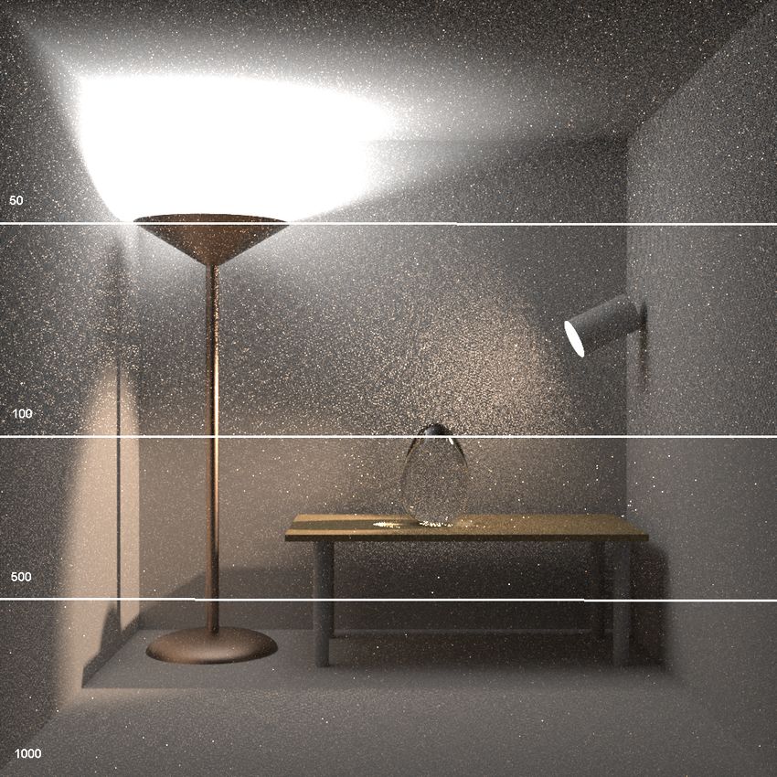
ii

PREFACE

First of all, I want to send a special thanks to my supervisor Professor Alessandro Foi,
who gave me a fascinating topic and also helped me achieve this thesis’s objective.
To make thesis possible, I also would like to thank Dr. Markku Mäkitalo, Prof. Pekka
Jääskeläinen, and M.Sc. Matias Koskela for helping me with the renderer and program-
ming problem.

Tampere, 4th April 2020

Duong Trung Kien
iii

CONTENTS

1 Introduction . . . . . . . . . . . . . . . . . . . . . . . . . . . . . . . . . . . . . . .   1
2 Path tracing . . . . . . . . . . . . . . . . . . . . . . . . . . . . . . . . . . . . . . .   2
   2.1 Brief history of path tracing . . . . . . . . . . . . . . . . . . . . . . . . . . .     2
   2.2 Path tracing algorithm . . . . . . . . . . . . . . . . . . . . . . . . . . . . . .      3
   2.3 Noise in path tracing . . . . . . . . . . . . . . . . . . . . . . . . . . . . . . .     4
3 Analysis method . . . . . . . . . . . . . . . . . . . . . . . . . . . . . . . . . . . .      6
   3.1 Random Variable . . . . . . . . . . . . . . . . . . . . . . . . . . . . . . . . .       6
   3.2 Sample mean, sample variance and sample standard deviation . . . . . . .                7
   3.3 Mean and variance of sample estimator . . . . . . . . . . . . . . . . . . . .           7
   3.4 Bias of estimator . . . . . . . . . . . . . . . . . . . . . . . . . . . . . . . . .     8
4 Implementation . . . . . . . . . . . . . . . . . . . . . . . . . . . . . . . . . . . . . 10
   4.1 Mitsuba versus pbrt-v3 . . . . . . . . . . . . . . . . . . . . . . . . . . . . . . 10
   4.2 Data and analysis program preparation          . . . . . . . . . . . . . . . . . . . . 13
5 Observation and evaluation . . . . . . . . . . . . . . . . . . . . . . . . . . . . . . 18
   5.1 Data observation . . . . . . . . . . . . . . . . . . . . . . . . . . . . . . . . . 18
   5.2 Data analysis . . . . . . . . . . . . . . . . . . . . . . . . . . . . . . . . . . . 22
6 Conclusion . . . . . . . . . . . . . . . . . . . . . . . . . . . . . . . . . . . . . . . 26
References . . . . . . . . . . . . . . . . . . . . . . . . . . . . . . . . . . . . . . . . . 27
iv

LIST OF SYMBOLS AND ABBREVIATIONS

   MVUE   minimum variance unbiased estimator
   PDF    probability density function
   spp    sample per pixel

1

1 INTRODUCTION

Path tracing is one of plenty techniques that can render a realistic image by mimicking
the physics of light propagation within a scene. Path tracing has a number of applications
in the film and game industry. For example, in the film industry, two famous movies of
Disney: A Bugs Life (1998) and Cars (2016) are made by path tracing (P. H. Christensen
and Jarosz 2016). The advantages of path tracing are the high-quality image and the
simplicity in the algorithm. Nowadays, path tracing remains in use in a brute-force way,
which causes the noise and the time-consuming. A 90-minute movie needs 130,000
high-resolution frames, and each frame needs millions of color pixels (P. H. Christensen
and Jarosz 2016). Therefore, the brute-force path tracing is not efficient enough for mak-
ing a computer-generated (CG) movie, and many evolutions of path tracing have been
developed. Different techniques can improve the performance as well as the quality of
the path tracing.

Rendering images offline, such as CG movies, is a simple task for path tracing. Whereas
nowadays real-time rendering, which is more complicated, is getting more research at-
tention, especially in game industry. Along with stories, gameplay, and the ideal of the
game, the graphic becomes a competitive factor in game industry. The demand for high-
quality graphics and rendering the image in real-time create challenges for path tracing.
In late 2018, NVIDIA released a graphics card, which can make real-time path tracing
rendering integrate with video games such as Battlefield 5, Minecraft, and Call of Duty:
Modern Warfare (Jones 2020). However, the cost of such a high-class graphic card is
over $1000 that is not affordable for everyone.

When upgrading the hardware is not possible, the improvement in software is significant.
Hence, the objective of this thesis is to study and understand the noise caused by ren-
dering the low ssp image. The thesis contains 6 chapters. Chapters 2 and 3 explain the
theories of path tracing and the mathematical method to study the noise. The implemen-
tation is proposed in Chapter 4, and Chapter 5 is observation and evaluation. Finally,
Chapter 6 summarizes the results and findings of the research.
2

2 PATH TRACING

Path tracing is an image rendering algorithm based on the Monte Carlo method for the
three-dimensional scenes using global illumination effects. Path tracing intends to render
an image that makes no distinction from photographs. Path tracing can simulate com-
plex phenomena, such as soft shadows, depth of field, and motion blur. However, this
method requires extremely high hardware capability and time to render a high-quality im-
age (Öqvist 2015). This chapter represents the essential concepts of the path tracing
method.

2.1 Brief history of path tracing
In the 1980s, due to the need for realistic image rendering in film, computer games,
and many other visual industries, the ray-tracing algorithm, introduced by Turner Whitted,
became the most popular algorithm in rendering (Dutre et al. 2016). It brought to light
the concept of ray tracing and later lead to path tracing algorithm. In nature, how animal
eyes or cameras capture the objects surrounding is that eyes receive light ray from the
environment. Ray-tracing is the reverse version of that process. Ray-tracing follows
the light beams, which entered the eyes, back to the light sources. This method was so
famous at that time because ray-tracing method can generate the reflection and refraction
effect and produce synthetic images with high quality and similar to photographs (Whitted
2018).

                     Figure 2.1. Ray-tracing diagram (Henrik 2009)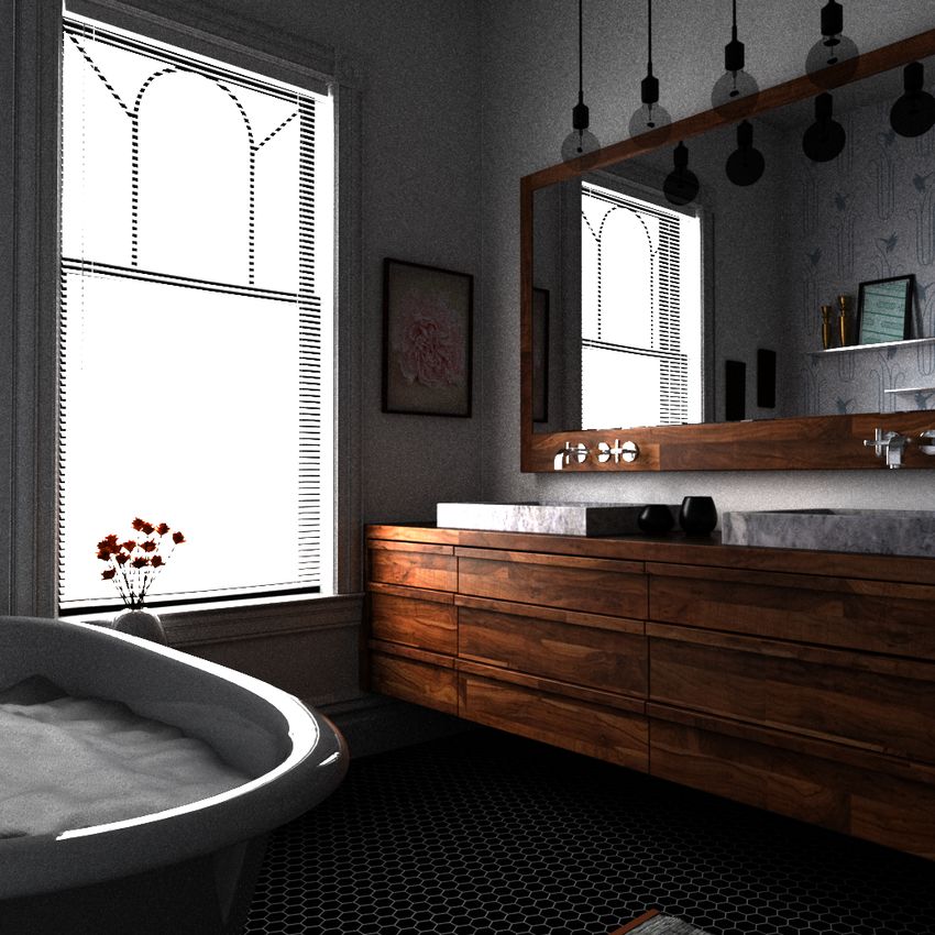
3

Although the quality of the output images of rays tracing is excellent, the rendering per-
formance is time-consuming because of the massive number of rays traced. Therefore,
many solutions to improve the performance of ray-tracing were proposed, including path
tracing (Dutre et al. 2016). Consequently, path tracing is one specific form of ray-tracing,
and both path tracing and ray-tracing are now being used widely in games, film, and many
other industries.

2.2 Path tracing algorithm
Firstly, how the ray-tracing algorithm can generate such a high-quality image is introduced
to understand the path tracing algorithm. A global illumination picture is synthesized by
calculating the radiance value Lpixel for each pixel of the image (Whitted 2018). This
value is measured by calculating the radiance value of the ray coming from the scene to
the camera (Whitted 2018). The best ways to demonstrate the process is by the equation
(2.1) and Figure 2.2:

                                     ∫︂
             L(x, w) = Le (x, w) +        L(h(x, w′ ), −w′ )fr (−w′ , x, w)cos(θ′ )dw′    (2.1)
                                      Ω

           Figure 2.2. Ray tracing set-up (Dimov, Penzov and Stoilova 2007)

where L(x, w) is the total spectral radiance, Le (x, w) is the emitted spectral radiance,
L(h(x, w′ ), w′ ) is the is spectral radiance toward the point h(x, w′ ) from direction w′ , and
fr (−w′ , x, w) is the bidirectional reflectance distribution function (BRDF) (Dimov, Penzov
and Stoilova 2007). From equation (2.1), global illumination image synthesis visibly de-
pends on two main factors: the position of the camera, and the direction of the camera.
In path tracing, the Monte Carlo sampling rule is used so that the rays distributes ran-
domly for each pixel and the number of random rays is equal for all pixels. Each beam
bounces for a certain amount of times either being entirely absorbed or entirely escaping
the scene, and then the radiance value is calculated based on all the objects colliding with
the ray (Öqvist 2015). Finally, the average of all sample values of each pixel represents
the color and the illuminance of that pixel (Öqvist 2015). Because of Monte Carlo sam-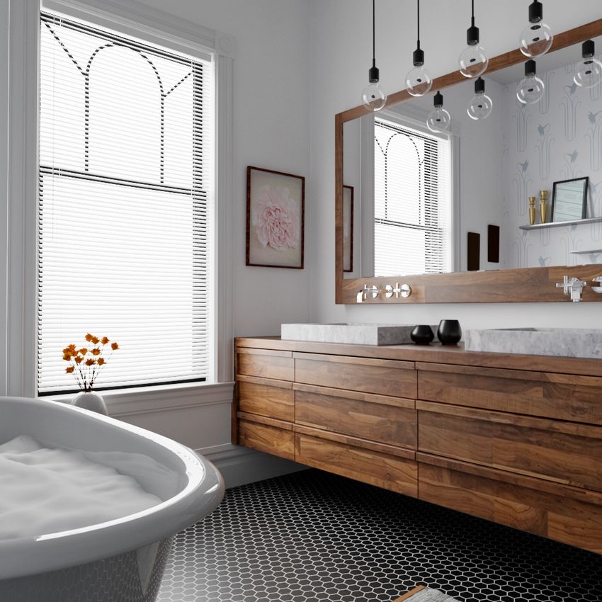
4

pling methods, which based on establishing random process, the resulting image often
contains noise, and the characteristics of noise are investigated in the following chapter.

2.3 Noise in path tracing
Although the path tracing algorithm can generate such a high-quality image, this algorithm
also needs a reasonable number of samples per pixel (spp) in order to work efficiently.
The path tracing method uses at least 100 spp to synthesize an image, which is the
unnoticeable amount of noise Jensen and N. J. Christensen 1995. The fewer number of
samples is used, the noisier image is. The noise effect occurs in images caused by the
independence of pixel synthesis. Indeed, each pixel’s color value is independent from the
neighbor, leading to the differences in hue, saturation, and lightness between each pixel
(Öqvist 2015). For example, Figure 2.3, the average value of pixel close to a small but
bright light source can be too high, because of the low probability for each sampled light
path to combine the light source (Öqvist 2015).

                Figure 2.3. Noise and light source relation (Öqvist 2015)

Figure 2.3 is the visual explanation for the assumption that the noise depends on the
spp. At 50 spp, the image is suffering from the white noise. However, the white noise
disappears when the number of samples increased, and the image is less noisy when
the spp reaches 1000.

Even such high samples can generate a noise-free image, this method is not feasible. In
practice, a reasonable number of spp is used in image rendering to balance the quality
of the image and the render performance. The most straightforward method to find the
sensible number of spp is to compute the standard deviations of pixels. When it is above a
5

threshold, more samples need to be added. This method can guarantee that the number
of rays used is optimal for an acceptable image Jensen and N. J. Christensen 1995.
6

3 ANALYSIS METHOD

The image needs to be analyzed pixelwise to identify the characteristics of the image
noise. Hence, the mean and standard deviations are sufficient tools to extract noise
information using the estimation theory. This chapter explains the primary theory about
estimation, mean, and standard deviation and how it can be applied in image processing.

3.1 Random Variable
By definition, every outcome of an experiment is a random variable (denoted X) (Pa-
poulis and Pillai 2002). In statistics, an observation is the value that actually obtained
from experiment (Papoulis and Pillai 2002). The population is the collection of all pos-
sible observations of the random variable, and the sample is a subset of the population
(Montgomery and Runger 1994). The population can be finite or infinite. In practice,
the observation of the entire population is unattainable, so the behavior of the sample
can decide the characteristics of the population (Montgomery and Runger 1994). In this
scope, each image is a random variable and population is all possible outcomes of the
image. Because the image can be rendered with unlimited random seeds, the population
is infinite.

The purpose of this experiment is to find the relation between the mean and the variance
of the images. Mean or expected value of a random variable (denoted µ) is the following
integral:                                        ∫︂   ∞
                               µ = E{x} =                 xf (x)dx                   (3.1)
                                                  −∞

where f (x) is the density function (Papoulis and Pillai 2002). The variance of random
variable (denoted σ) is computed by the formula:
                                      ∫︂   ∞
                                 2
                                σ =            (x − µ)2 f (x)dx                      (3.2)
                                        −∞

where µ is the mean from equation (3.1). Comparing equation (3.1) and equation (3.2),
the variance of random variable is the mean of the variable {(x − µ)2 }. Then the variance
of random variable can be computed:

                                     σ 2 = E{(x − µ)2 }                              (3.3)
7
and the standard deviation is the square root of the variance (Papoulis and Pillai 2002).
However the population is infinite, the population mean and population variance cannot
be calculated directly from above equations. In this project, the sample mean (denoted
X) and sample standard deviation (denoted S) are used to estimate the population mean
(µ) and population standard deviation (σ).
3.2 Sample mean, sample variance and sample standard
deviation
The sample mean is the sum of all values divided by the number of values in the data set.
For example, the collection of numbers: X1 , X2 , X3 , . . . , Xn have the mean calculated by:
n
1 ∑︂ X1 + X2 + X3 + · · · + Xn
X= Xi = (3.4)
n n
i=1
Besides, the sample mean is necessary to compute the sample variance and sample
standard deviation value, which play an essential role in data analysis and image pro-
cessing. The computation of sample variance is straightforward with three steps. The
first step is computing the sample mean value with equation (3.4). The next step is to
subtract the sample mean from values in the set and take the resulting square. Finally,
the sample variance is the average value. The formulas below describe examples of
computing the sample variance of the set of number: X1 , X2 , X3 , . . . , Xn
∑︁n
2 i=0 (Xi− X)2
S = (3.5)
n−1
and the sample standard deviation of the set of number: X1 , X2 , X3 , . . . , Xn
√︄
∑︁n
− X)2
i=0 (Xi
S= (3.6)
n−1
where n is the number of numbers in the set, and X is the mean of that set.
While the sample mean value represents the center of the data collection, both the sam-
ple variance and the sample standard deviation describe the dispersion of a data set. In
other words, the low standard deviation value means that data values tend to close to the
mean value, and high standard deviation value means that data values are far from the
mean value (Montgomery and Runger 1994).
3.3 Mean and variance of sample estimator
In signal processing, many systems use estimation theory as the core to extract the in-
formation (Kay 1993). Estimation theory intends to take out the estimation values of a8
group of parameters. In this project, the mean and the standard deviation of pixel are
sample data, which are used to find the relation between the population mean and the
population standard deviation. Because the estimators are also random variable the def-
inition of mean and variance of an estimator need to be defined. The expected value of a
random variable is the mean of that variable (Montgomery and Runger 1994). According
to equation (3.1), the mean of the estimator is the expected value of the estimator:
µθˆ︁ = E(θ)
ˆ︁ (3.7)
where µθˆ︁ is mean of the estimator, E(θ)
ˆ︁ is the expected value of the estimator of pa-
rameter θ. Using equation (3.3) and equation (3.7), The variance of sample estimator
is:
ˆ︁ 2
σθ2ˆ︁ = E[θˆ︁ − E(θ)] (3.8)
where σ 2ˆ︁ is the variance of estimator, and θˆ︁ is the estimator of the parameter θ
θ
3.4 Bias of estimator
In statistics, an "accurate" estimator does not neither overestimate nor underestimate,
and an estimator called biased when it becomes overestimated or underestimated (Mont-
gomery and Runger 1994). The different between estimated value and the true value is
the bias of the estimator:
b(θ) ˆ︁ − θ = 0
ˆ︁ = E(θ) (3.9)
where b(θ)
ˆ︁ is the bias of the estimator, E(θ)
ˆ︁ is the expected value of the estimator, and θ
is the parameter. As mentioned previously, the expected value of random variable is the
mean of the variable. Therefore, the expected value, E(Xi ), of a set of random variable
X1 , X2 , X3 , . . . , Xn is the population mean µ. Sample mean is the unbiased estimator of
population mean that can be proved:
n
1 ∑︂
E(X) = E( Xi )
n
i=1
n
1 ∑︂
= E(Xi )
n (3.10)
i=1
n
1 ∑︂
= µ
n
i=1
=µ9
Consider the sample variance:
∑︁n
2 i=1 (Xi − X)2
E(S ) = E( )
n−1
n
1 ∑︂
= E (Xi − X)2
n−1
i=1
n
1 ∑︂ 2
= E Xi2 + X − 2Xi X (3.11)
n−1
i=1
n
1 ∑︂ 2
= E Xi2 − nX
n−1
i=1
n
1 ∑︂ 2
= [ E(Xi2 ) − nE(X )]
n−1
i=1
2 σ2
Since E(Xi2 ) = µ2 + σ 2 and E(X ) = µ2 + n (Montgomery and Runger 1994):
n
2 1 ∑︂ 2 σ2
E(S ) = [ µ + σ 2 − n(µ2 + )]
n−1 n
i=1
1 (3.12)
= [nµ2 + nσ 2 − nµ2 − σ 2 ]
n−1
= σ2
Aligned with above ascertainment, the sample mean and sample variance are the unbi-
ased estimators of population mean and population variance (Montgomery and Runger
1994). Therefore, the sample mean and the sample variance of pixel are the accurate
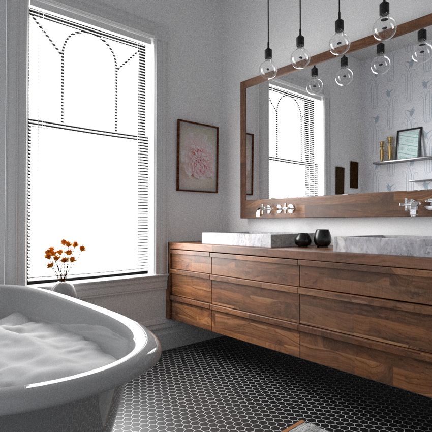
estimators of the mean and the variance of the unlimited population of images.10 4 IMPLEMENTATION This chapter shows how the noise in an image is generated by the path tracing algorithm that is analyzed using renderer and Python programming language. Two main imple- mentations are introduced in this chapter. Firstly, the renderers are introduced, which are Mitsuba renderer (Jakob 2020) and pbrt-v3 renderer (Pharr, Humphreys and Wen- zel 2015), and the reason why pbrt-v3 renderer is chosen. Secondly, the data analysis program written in Python is demonstrated. 4.1 Mitsuba versus pbrt-v3 In this project, two different renderers, Mitsuba and pbrt-v3, were used to render images. Both renderers have the same setting options base on path tracing algorithms such as maximum depth, Russian Roulette depth, spp, and scramble value. Moreover, the image quality of the two renderers is not distinguishable. Figure 4.1. Bathroom image with 2048 spp 17 bounces Mitsuba left, and 2048 spp 4 bounces pbrt-v3 right. The two images in Figure 4.1 have the same quality, and the difference between the two images is the brightness because of the level of ray bounces per pixel. Thus, the control of the depth for each pixel is critical.
11
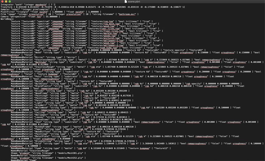
Figure 4.2. Mitsuba configuration
Figure 4.3. Pbrt-v3 configuration
According to Figure 4.2 and Figure 4.3, Mitsuba has a conducive user-interface while
pbrt-v3 uses a script file as scene-setting. Therefore, it is quite challenging for a new
user to get familiar with pbrt-v3. Moreover, pbrt-v3 has to be complied with by the source12
code on git, while Mitsuba is a software for Windows, Mac os, and Linux so that it is
much more difficult to start with the pbrt-v3 than the Mitsuba. However, it is not a serious
hindrance to pbrt-v3 thanks to the detailed documentation of pbrt-v3.
The reason why pbrt-v3 is appropriate for analysis is the flexibility of the pbrt-v3. The
noise needs to be analyzed base on spp, the depth of each pixel, and the illumination
characteristic of different scenes. With Mitsuba renderer, there is no way to extract the
depth of the ray from the software. The statistic log only shows the average depth for all
pixel image, but the image has to be investigated pixelwise. The source code accessibility
of pbrt-v3 is the solution to that problem. The number of bounces of each pixel can be
stored into a 2D vector by modifying the source code.
1 i f ( rendering ) {
2 i n t x = ( i n t ) sampler . r e t u r n x ( ) + 1 ;
3 i n t y = ( i n t ) sampler . r e t u r n y ( ) + 1 ;
4 depthData [ y ] [ x ] = bounces ;
5 }
6
7 return L ;
Program 4.1. Map bounces into 2D vector.
Then in the render process, when all the depths of the whole image are entirely encap-
sulated, the data is exported and saved in a CSV file.
1 std : : ofstream ofs ;
2 o f s . open ( " image−depth . csv " , s t d : : o f s t r e a m : : app ) ;
3 f o r ( s t d : : v e c t o r < i n t > row : depthData ) {
4 std : : ostringstream vts ;
5
6 i f ( ! row . empty ( ) ) {
7 // Convert all but the last element to avoid a trailing ","
8 s t d : : copy ( row . begin ( ) , row . end ( ) − 1 ,
9 s t d : : o s t r e a m _ i t e r a t o r < i n t >( v t s , " , " ) ) ;
10
11 // Now add the last element with no delimiter
12 v t s13
lack of memories can be solved by the portable hard drive and Google drive. Regarding
all listed reasons, pbrt-v3 is the most appropriate choice.
Figure 4.4. Bounces map result.
4.2 Data and analysis program preparation
In this experiment, more than 100 images per model need to be examined. Several im-
ages, which have the same configuration, such as spp, depth, camera position, sampler,
and model, are generated. Despite the similarity in the setting, the image differed each
time it is created. The reason for the differences is the Monte Carlo sampling algorithm,
which generates noise in the image, and the mission is to investigate the noise’s behav-
iors. Rendering the image one by one is time-consuming and inefficient. Correspondingly,
the first step is to build an automated image render system. In macOS or Linux, the script
file is used to render the images by a for loop:
1 f o r i i n { 1 . . numberOfPic } ;
2 do
3 . / p b r t path−t o / scene . p b r t
4 mv data / image−depth . csv data / picName$ { i } . csv
5 mv data / picName . e x r data / picName$ { i } . e x r
6 done
Program 4.3. Automated rendering script.
where scene.pbrt is the file contains all the settings.
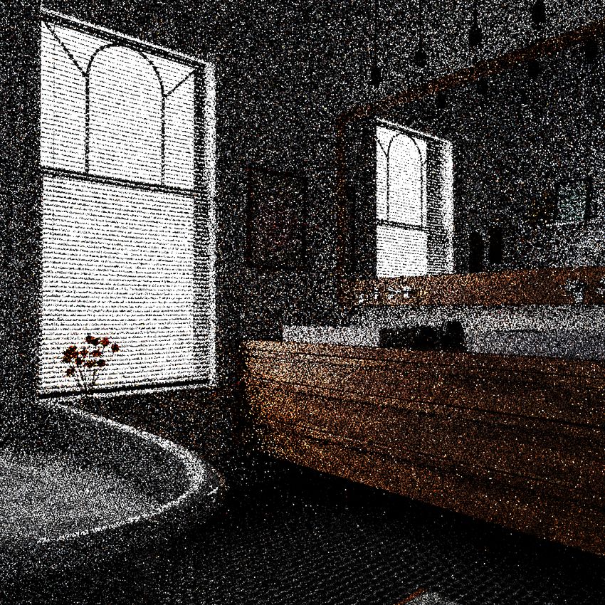
Figure 4.5 indicates an example of images rendered from the bathroom scene with 1
spp. Comparing to the result in Figure 4.1, Figure 4.5 is much noisier, because it was
only sampled with 1 spp. Image with high spp has less noise but takes much more time
to synthesize (Öqvist 2015). According to the experiment, with the same resolution, a
2048-spp image takes approximately 3 hours to process, while 1-spp image finishes in
only 30 seconds.14
Figure 4.5. Two images with 1 spp and max-depth 17
The two images in Figure 4.5 seem to be the same, but in fact, they are two different
images. Taking a closer look, Figure 4.6 represents the images that are 100x100 pixel
top left corner of images in Figure 4.5, respectively. When comparing the two images,
there are differences in the position of the noise and the color of dots. Therefore, 200
images of each different spp, max depth, and the scene were rendered to study the
behaviors of noise in path tracing.
Figure 4.6. 1-spp images comparison.
Program 4.4 is the analysis program written in Python. As specified in the program, the
images were detached into three channels: red, green, and blue, then put into a 3D array
(Figure 4.7). The following step is to compute the mean and the standard deviation of
each pixel vector, which has the direction illustrated in Figure 4.7. Then the result has the
same resolution with the image.15
Figure 4.7. Stack images diagram.
After flattening the result matrices and plot, the plot in Figure 4.8 shows the standard
deviation over the mean for the red, green, and blue channels. Combining the depth
status of each image prepared earlier, it is now ready for evaluating in the next chapter.
Figure 4.8. Mean and standard deviation of 150-stack-images.
1 #!/usr/bin/env python3
2 # -*- coding: utf-8 -*-
3 """
4 Created on Mon Jan 27 13:35:27 2020
5
6 @author : kienduong
7 """16 8 9 import OpenEXR 10 from PIL import Image 11 import numpy as np 12 from numpy import random as np_random 13 import a r r a y 14 import m a t p l o t l i b . p y p l o t as p l t 15 import m a t p l o t l i b . image as mpimg 16 import Imath 17 18 / / open 2048 spp image and g e t i t s i z e 19 f i l e _ 2 0 4 8 = OpenEXR . I n p u t F i l e ( " bathroom1 . e x r " ) 20 dw = f i l e _ 2 0 4 8 . header ( ) [ ’ dataWindow ’ ] 21 s i z e = ( dw . max . x − dw . min . x + 1 , dw . max . y − dw . min . y + 1 ) 22 FLOAT = Imath . P i x e l T y p e ( Imath . P i x e l T y p e . FLOAT) 23 (R, G, B) = [ a r r a y . a r r a y ( ’ f ’ , f i l e _ 2 0 4 8 . channel ( Chan , FLOAT ) ) 24 . t o l i s t ( ) f o r Chan i n ( "R" , "G" , "B" ) ] 25 R_r = np . r e s i z e (R, ( s i z e [ 1 ] , s i z e [ 0 ] ) ) 26 G_r = np . r e s i z e (G, ( s i z e [ 1 ] , s i z e [ 0 ] ) ) 27 B_r = np . r e s i z e ( B , ( s i z e [ 1 ] , s i z e [ 0 ] ) ) 28 pic_2048 = np . d s t a c k ( ( R_r , G_r , B_r ) ) 29 30 num_pics = 100 31 32 / / c r e a t e empty 3D a r r a y f o r 3 chanel red , green and b l u e 33 stack_images_R = np . empty ( ( s i z e [ 1 ] , s i z e [ 0 ] , num_pics ) ) 34 stack_images_G = np . empty ( ( s i z e [ 1 ] , s i z e [ 0 ] , num_pics ) ) 35 stack_images_B = np . empty ( ( s i z e [ 1 ] , s i z e [ 0 ] , num_pics ) ) 36 37 / / read images and add t h e p i x e l v a l u e t o t h e empty s t a c k 38 f o r x i n range ( 0 , num_pics ) : 39 p i c = OpenEXR . I n p u t F i l e ( " bathroom " + s t r ( x + 1 ) + " . e x r " ) 40 (R, G, B) = [ a r r a y . a r r a y ( ’ f ’ , p i c . channel ( Chan , FLOAT ) ) 41 . t o l i s t ( ) f o r Chan i n ( "R" , "G" , "B" ) ] 42 R_r_1 = np . r e s i z e (R, ( s i z e [ 1 ] , s i z e [ 0 ] ) ) 43 G_r_1 = np . r e s i z e (G, ( s i z e [ 1 ] , s i z e [ 0 ] ) ) 44 B_r_1 = np . r e s i z e ( B , ( s i z e [ 1 ] , s i z e [ 0 ] ) ) 45 stack_images_R [ : , : , x ] = R_r_1 46 stack_images_G [ : , : , x ] = G_r_1 47 stack_images_B [ : , : , x ] = B_r_1 48 49 / / c a l c u l a t e t h e mean and s t a n d a r d d e v i a t i o n o f each s t a c k c o r r e s p o n d i n g t o a x i s 2 50 m_r = np . mean ( stack_images_R , a x i s =2) 51 c _ r = np . s t d ( stack_images_R , a x i s =2) 52 m_g = np . mean ( stack_images_G , a x i s =2) 53 c_g = np . s t d ( stack_images_G , a x i s =2) 54 m_b = np . mean ( stack_images_B , a x i s =2) 55 c_b = np . s t d ( stack_images_B , a x i s =2) 56 57 / / f l a t t h e data and p l o t 58 m _ f l a t _ r = m_r . f l a t t e n ( ) 59 c _ f l a t _ r = c_r . f l a t t e n ( )
17

60   p l t . p l o t ( m_flat_r , c_flat_r ,          ’ r + ’ , markersize =0.1)
61
62   m _ f l a t _ g = m_g . f l a t t e n ( )
63   c _ f l a t _ g = c_g . f l a t t e n ( )
64   p l t . p l o t ( m_flat_g , c _ f l a t _ g ,   ’ g+ ’ , m a r k e r s i z e = 0 . 1 )
65
66   m _ f l a t _ b = m_b . f l a t t e n ( )
67   c _ f l a t _ b = c_b . f l a t t e n ( )
68   p l t . p l o t ( m_flat_b , c _ f l a t _ b ,   ’ b+ ’ , m a r k e r s i z e = 0 . 1 )
69   p l t . show ( )

                                         Program 4.4. Image analysis program.
18
5 OBSERVATION AND EVALUATION
Observation and analysis are the two most critical and demanding tasks of studying the
noise behaviors. The chapter is divided into two parts: data observation and data analy-
sis. In the observation part, the images and the bounces were observed and investigated,
then the general statements about the observation were given. Based on the general idea
obtained from the observation, the analysis step studies more deeply about the statistics
of the images pixelwise, which are the sample mean and the sample standard deviation.
This chapter aims to answer two questions: whether there is a function of mean and
standard deviation of pixel
σ = g(µ) (5.1)
where σ is the population standard deviation, µ is the population mean and g is the
function, and whether the function holds under special conditions.
5.1 Data observation
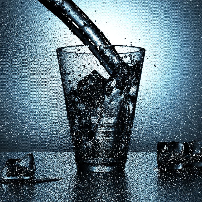
Three different models, which are from the open source of Benedikt Bitterli (Bitterli 2016),
were used in this project: glass-of-water, veach-bidir, and bathroom. Figure 5.1 is the
example images rendered by those models in 4096 spp. The models were chosen with
the increasing rate of reflection, refraction, and decrease in the number of light sources.19
(a) Veach-bidir (b) Bathroom
(c) Glass-of-water
Figure 5.1. High quality image rendered by three models
According to Figure 5.1, the veach-bidir scene has nearly no reflection and refraction,
and two light sources. Although the bathroom has only one light source, which is the
window, the bathroom scene’s total illuminance level is higher than the veach-bidir. The
phenomenon occurs because the light direction of two lamps is into the corner, while
the window direction is direct to the room. Moreover, the glass in the bathroom also
reflects the light causing the high brightness. Although the glass-of-water scene has
much refraction and reflection, there is no light source in the scene so that the scene’s
presence is dim.20
(a) Veach-bidir 1 spp (b) Bathroom 1 spp (c) Glass-of-water 1 spp
Figure 5.2. Images render with 1 spp
Figure 5.2 is an example of three 1-spp images of three models. With the unlimited num-
ber of bounces for each ray, the veach-bidir is much noisier comparing to other models.
The top right corner is too bright, while the rest of the picture lacks of light, and the object
on the table disappears. The same effect happens with the bathroom floor and ice cube
in the glass-of-water scene. This phenomenon is unavoidable in the low-spp images,
and this is not the problem concerned. The problem to be concerned about is the func-
tional relation between the mean and the standard deviation in special condition, which
is number of bounces.
After generating the CSV file for the image bounces, an additional Program 5.1 is needed
to plot the CSV file as an image, Figure 5.3. Although the bounces-images in Figure
5.3 are synthesized from two different images, those plots are approximately the same.
Some pixels have a different number of bounces, but this number is small and trivial. Con-
sequently, the bounce, which is the mean of all bounces-image, used for the experiment
is the same for all image.21
Figure 5.3. Bounces-images, where horizontal axis and vertical axis are index of pixel
and the color bar represents the number of bounces by color22
1 import csv
2 import numpy as np
3 import m a t p l o t l i b . p y p l o t as p l t
4
5 w i t h open ( " room " + s t r ( 1 ) + " . csv " ) as c s v f i l e :
6 csvdata = csv . r e a d e r ( c s v f i l e , d e l i m i t e r = " " , quotechar = " | " )
7 data = [ ]
8 f o r row i n csvdata :
9 data . append ( np . f r o m s t r i n g ( row [ 0 ] , dtype= i n t , sep= ’ , ’ ) )
10 p l t . imshow ( data , vmin =0 , vmax=34 , cmap= " j e t " , aspect = " auto " )
11 p l t . colorbar ( )
12 p l t . show ( )
Program 5.1. Bounces plot program.
5.2 Data analysis
The data can be stored and evaluated in several methods. Different data structures have
the optimal analysis performance with different shapes of data. The images need to be
stacked in a 3D-array, to calculate the statistics of the images pixelwise. In addition, there
are three different channels: R, G, and B in an image, so the solution is three 3D-arrays
for each one, and each channel is evaluated separately. The form of the data structure is
described in Figure 4.7. The first dimension and the second dimension refer to coordinate
x and y of the image, respectively, and the third dimension is the number of images. The
mean and the standard deviation of the data container are computed and plotted for the
third dimension. The plots of three models with 8 spp are showed in Figure 5.4, where
the x-axis is the sample mean, and the y-axis is the sample standard deviation.
(a) Veach-bidir statistics (b) Bathroom statistics (c) Glass-of-water statistics
Figure 5.4. images statistics, where horizontal axis is the mean and vertical axis is the
standard deviation.
Figure 5.4a of Veach-bidir scene is in a short-range and impossible to do the evaluation
compare to other scenes. This phenomenon caused by the high contrast in the image,
Figure 5.2a. Because of that reason, the Veach-bidir scene was not able to do any
further experiments. Although, the Figures 5.4b and 5.4c look interesting, the plots are
still confused and chaotic. The images were rendered in the resolution of 1024x1024,
so there were over million points on the plot. For better visualization, the data needs to
be sliced into small pieces. The number of bounces was used to classify the data. The23
bounces were broken down into intervals in the range from 0 to the maximum bounces
per pixel, and the pixels in the same interval are in the same group. The subsets of data
were processed and plotted in the same way, and the results are in Figure 5.5
(a) 0 to 1.5 (b) 1.5 to 3 (c) 3 to 4.5
(d) 4.5 to 6 (e) 6 to 7.5 (f) 7.5 to 9
(g) 9 to 10.5 (h) 10.5 to 12 (i) 12 to 13.5
(j) 13.5 to 15 (k) 15 to 16.5 (l) 16.5 to 18
Figure 5.5. Bathroom image statistics in the interval of 1.5 bounces, where horizontal
axis is the mean and vertical axis is the standard deviation.
If the images in Figure 5.5 are stacked, the outcome is the Figure 5.4b. With the subplots,
Figure 5.5, the statistics of images can be investigated at the micro-level without any
modification. The same experiment was applied with the glass-of-water scene to ensure
that the subplot’s behavior is consistent.24
(a) 0 to 2 (b) 2 to 4 (c) 4 to 6
(d) 6 to 8 (e) 8 to 10 (f) 10 to 12
(g) 12 to 14 (h) 14 to 16 (i) 16 to 18
(j) 18 to 20 (k) 20 to 22 (l) 22 to 24
(m) 24 to 26 (n) 26 to 28 (o) 28 to 30
Figure 5.6. Glass-of-water image statistics in the interval of 2 bounces, where horizontal
axis is the mean and vertical axis is the standard deviation.
According to Figure 5.4, 5.5, and 5.6, the data is consistent with all models after the sub-
set partition. Although the data was split into subsets, the graph is messy and impossible
to examine. There are over million sample need to be studied, but with that partition
method, the average samples per subplot are more than 30000 each. In fact, the number25 of bounces from 0 to 4 accounts for the majority, the subplot in range 0 to 4 has ap- proximately 800000 pixels, 80 percent number of pixels, while the other subsets occupy only 20 percent. There is no difference between studying a graph of 1 million points and a graph of 800000 points. Both graphs are too condensed, so it is impractical to learn any sufficient information about the noise model. The data needs to be classified with another method for visualization. However, this thesis does not cover further experiments because it is over the scope of a Bachelor thesis.
26

6 CONCLUSION

The research aimed at understanding the noise model in path tracing, by estimating the
relation between the mean and standard deviation of pixel. The purpose of investigating
the noise in path tracing is to discover the noise model to apply for further development
of the path tracing algorithm. The research indicated that path tracing is an emerging
algorithm and a wide field for development. Noise cannot be eliminated entirely, so the
behavior of noise is beneficial for noise filtering. The thesis has shown the basic concept
of path tracing, noise in path tracing, and how the experiment is processed step by step.

Different renderers and analysis methods were used in order to obtain the correct esti-
mators for the noise model. The data was observed in a way that the number of bounces
was in a specific range for each set. However, due to the massive amount of data and
the data confusion, the experiment has not had the final answer yet. It does not mean
that we have not gained anything during the research. The suitable render pbrt-v3 was
modified to give more detailed information about the image. Furthermore, the images or
data were correctly rendered to be ready for future research.

The obstacles, such as choosing the renderer, and analysis method, were the most time-
consuming part of the research. Choosing and modifying the renderer are significant
problems while doing the preparation. The renderer needs to be adjusted to extract the
ray bounces for each pixel while keeping the quality of the image. This step requires a
strong knowledge of technology, C++, and Os. The analysis method was also a significant
puzzle that needed to be solved. The size of data is too large for observation, so the data
was sliced into a small subset. The bounces-files extracted by modifying the renderer
were used in the data partition, but the data is still disordered and hard to visualize.

In general, the conclusion of the noise model cannot be obtained. Understanding the
noise model of an algorithm is a complicated task and cannot be covered entirely. More
experiments need to be conducted to get a conclusive and accurate statement about the
noise model.
27

REFERENCES

Christensen, P. H. and Jarosz, W. (2016). The Path to Path-Traced Movies. Foundations
  and Trends in Computer Graphics and Vision. Now Publishers Inc.
Jones, R. (2020). What is ray tracing? The PS5 and Xbox Series X feature explained.
  URL :   https://www.trustedreviews.com/news/nvidia-ray-tracing-3638206 (visited
  on 04/01/2020).
Öqvist, J. (2015). Path Tracing. URL: https://chunky.llbit.se/path_tracing.html
  (visited on 02/25/2020).
Dutre, P., Bala, K., Bekaert, P. and Shirley, P. (2016). Advanced Global Illumination. A K
  Peters, Ltd.
Whitted, T. J. (2018). A Ray-Tracing Pioneer Explains How He Stumbled into Global Illu-
  mination. URL: https://blogs.nvidia.com/blog/2018/08/01/ray-tracing-global-
  illumination-turner-whitted/ (visited on 02/27/2020).
Henrik (2009). Ray trace diagram. URL: https://commons.wikimedia.org/wiki/File:
  Ray_trace_diagram.svg (visited on 06/15/2020).
Dimov, I. T., Penzov, A. A. and Stoilova, S. S. (2007). Parallel Monte Carlo Sampling
  Scheme for Sphere and Hemisphere. Numerical Methods and Applications. Springer-
  Verlag Berlin Heidelberg.
Jensen, H. W. and Christensen, N. J. (1995). Optimizing Path Tracing using Noise Re-
  duction Filters. Proceedings of Winter School of Computer Graphics and Visualization
  95.
Papoulis, A. and Pillai, S. U. (2002). Probability, Random Variables, and Stochastic Pro-
  cesses. McGraw Hill.
Montgomery, D. C. and Runger, G. C. (1994). Applied Statistics and Probability for Engi-
  neers. John Wiley & Sons, Inc.
Kay, S. M. (1993). Fundamentals of Statistical Signal Processing: Estimation Theory.
  Prentice-Hall, Inc.
Jakob, W. (2020). Mitsuba 2: A Retargetable Forward and Inverse Renderer. URL: https:
  //mitsuba2.readthedocs.io/en/latest/src/getting_started/intro.html (visited
  on 03/10/2020).
Pharr, M., Humphreys, G. and Wenzel, J. (2015). Pbrt. URL: https://www.pbrt.org/
  index.html (visited on 03/10/2020).
Bitterli, B. (2016). Rendering resources. https://benedikt-bitterli.me/resources/. (Visited
  on 01/20/2020).
You can also read


