Z folding aircraft electromagnetic scattering analysis based on hybrid grid matrix transformation - Nature
←
→
Page content transcription
If your browser does not render page correctly, please read the page content below
www.nature.com/scientificreports
OPEN Z‑folding aircraft electromagnetic
scattering analysis based on hybrid
grid matrix transformation
Zeyang Zhou* & Jun Huang
To study the electromagnetic scattering characteristics of a morphing aircraft with Z-folding wings, a
method of hybrid grid matrix transformation (HGMT) is presented. The radar cross-section (RCS) of the
aircraft in the four Z-folding modes is calculated and analyzed. When considering the deflection of the
outer wing separately, the RCS of the wing under the head and side azimuth shows obvious dynamic
characteristics, while the peak and fluctuation range are quite different. When the mid wing and the
outer wing are deflected upwards together, the RCS of the aircraft under the positive side direction
could be significantly reduced. When the mid wing deflects upward and the outer wing remains level,
the peak of the side RCS of the aircraft is slightly reduced. When the mid wing deflects upwards and
the outer wing deflects downwards, this peak indicator is further reduced, while the local fluctuation
of the side RCS of the aircraft is increased. The HGMT method is effective to study the electromagnetic
scattering characteristics of the Z-folding aircraft.
With the increasing demand for multi-tasking, covert investigation and efficient flight, research on the aero-
dynamics, aero elasticity, stealth requirements and material structure of morphing aircraft has gained a lot of
attention1,2. Common variants include changes in wing length, increased sweep angle, variable area, and wing
folding3,4. The deformation causes a direct change in the shape of the aircraft, which in turn affects the aerody-
namic characteristics and stealth p erformance5. Facing the complex radar detection threats in the future battle-
field, the research on the electromagnetic scattering characteristics of morphing aircraft has important practical
significance and engineering value.
In the early design and application, the droppable nose of the aircraft provided the pilot with a good field of
vision during the take-off and landing phases. Other discrete deformations included active elastic wings, vari-
able wingspan and retractable landing gear. An aircraft with foldable wings was presented, which could switch
between long-term flight and high-speed movement modes6,7, at the same time, the stealth design of aircraft
was also considered. The emergence of variant technology was expected to improve flight performance, expand
the flight envelope, replace the traditional control surface and improve stealth p erformance8,9. A neutral point
was repositioned on the opposite wing, which was close to the hinge point of the wing above the actual center of
gravity10. According to the needs of the flying mission at the time, the Z-shaped wings of the morphing aircraft
could be folded into different configurations. Unstructured grids were used to discretize object shapes, and the
flow field of the aircraft after the wings were folded is s olved11,12, while different folding angles made the ability of
the wing to deflect the incident wave different. A bionic bird-wing folding aircraft was presented, where the outer
end of the wing could be contracted and expanded, resulting in a change in the plane shape of the w ing13. Using
high-speed video and flow field to measure the movement of the wing, when the stroke amplitude was increased,
there was a "flapping and throwing" action on the outside of the wing14. A combined deformation design was
investigated in detail, including the extension of the outer end of the wing and the increase in the sweep angle15.
It was worth noting that the change of the wingspan would affect the illumination area under the incident wave
from the head, and the change of the sweep angle would affect the deflection effect of the given incident wave.
The aerodynamic and stealth characteristics of the deformed aircraft would be changed, and how the continu-
ous deformation process dynamically affected electromagnetic scattering was worth exploring. When the sweep
angle of the wings of the aircraft increased, the projection of the entire machine in the direction of the body axis
was constantly decreasing16. Research on wing deformation, active elasticity and smart wing further promoted the
development of variant aircraft t echnology17. High-precision unstructured grids were used to process the target
surface, and physical optics (PO) and physical theory of diffraction (PTD) were used to calculate the radar cross
section18. The Z-shaped wing was designed and studied, and then used on high-altitude solar-powered morphing
School of Aeronautic Science and Engineering, Beihang University, Beijing 100191, China. *email: zeyangzhou@
buaa.edu.cn
Scientific Reports | (2022) 12:4452 | https://doi.org/10.1038/s41598-022-08385-9 1
Vol.:(0123456789)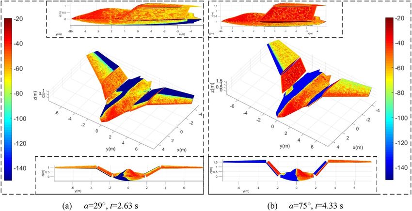
www.nature.com/scientificreports/
Figure 1. Schematic of dynamic scattering of the morphing aircraft with Z-folding wings.
aircraft19,20, while variation of electromagnetic scattering intensity on the surface of the panel at the outer end of
the large deformation wing would be very obvious. The ranking factor was used to filter an optimal solution for
the stealth design of a flying wing exhaust system21. The aerodynamic lift, drag and velocity distributions of the
variant aircraft in the two sweep modes were analyzed and discussed22. When there were geometrically complex
scattering obstacles, ray tracing became expensive or difficult to h andle23,24. The measurement algorithm of the
wing folding angle based on the three-axis accelerometer was designed, and the attitude of the fuselage and the
wing relative to the reference coordinate system was accurately c alculated25. The multi-rotor dynamic scattering
calculation method was presented to solve the radar stealth characteristic change of the compound helicopter26.
The control problem of a variable-swept wing deformed aircraft was studied, where the nonlinear switching sys-
tem and adaptive dynamic programming were p resented27. Damage sensing and self-healing magnetic polymer
composites had been studied. This new collaborative method could be applied to the deformation applications
of adaptive wing s tructures28,29. Compared with the high-speed rotating rotor, the folding movement of the
Z-shaped wing could be regarded as a slow small-angle rotation movement.
In general, the research on morphing aircraft technology has made substantial progress in many aspects,
including aeroelastic analysis, active torsion, and sweep angle changes, folding wings, dynamic models, sliding
skin and control technology. For Z-shaped wings, the folding of the middle and outer wings will increase the
side projection of the aircraft, which will adversely affect its stealth characteristics, while these effects and the
dynamic changes of the radar cross section still need to be explored and studied. Therefore, this article attempts
to present a hybrid grid matrix transformation method to evaluate the RCS changes brought to the aircraft
when the Z-wing is folded. The dynamic effects of multiple folding modes on the electromagnetic scattering
characteristics of aircraft will be investigated and discussed. Studying the dynamic scattering of the Z-folding
wing is of great importance and engineering value for the stealth design and development of morphing aircraft.
In this manuscript, the HGMT method is presented in “Hybrid grid matrix transformation”. Model of the
morphing aircraft is given in “Model”. Related results of aircraft RCS are discussed in “Results and discussion”.
Finally, the full text is summarized.
Hybrid grid matrix transformation
The schematic diagram of the dynamic electromagnetic scattering of the aircraft in different folding modes is
shown in Fig. 1, where Ar1 is the deflection angle of outer wing 1, Am1 is the deflection angle of mid wing 1, α
represents the azimuth angle between the radar station and the aircraft, β is elevation angle between the radar
station and the aircraft, Ar2 is the deflection angle of outer wing 2, Am2 is the deflection angle of mid wing 2. In the
current coordinate system, the middle wing remains level and the outer wing deflects downward when the aircraft
is flying in Z1 mode. For Z2 mode, the outer wing is fixedly attached to the middle wing and deflects upwards
together. In Z3 mode, the middle wing deflects upwards while the outer wing remains level. When the aircraft
is flying in Z4 mode, the middle section wing deflects upward and the outer section wing deflects downward.
Hybrid grid matrix. In the current observation field, the grid matrix of the aircraft could be expressed as a
hybrid form of the following matrices:
(1)
M a (ma (t)) = M r1 (mr1 (t)), M r2 (mr2 (t)), M w1 (mw1 (t)), M w1 (mw2 (t)), M f (mf (t))
where t is time, ma represents the aircraft model, mw1 is the model of mid wing 1, mw2 is the model of mid wing
2, mf is the model of fuselage, Ma is the grid coordinate matrix of ma, mr1 is the model of outer wing 1, Mr1 is the
grid coordinate matrix of outer wing 1, mr2 is the model of outer wing 2, Mr2 is the grid coordinate matrix of
Scientific Reports | (2022) 12:4452 | https://doi.org/10.1038/s41598-022-08385-9 2
Vol:.(1234567890)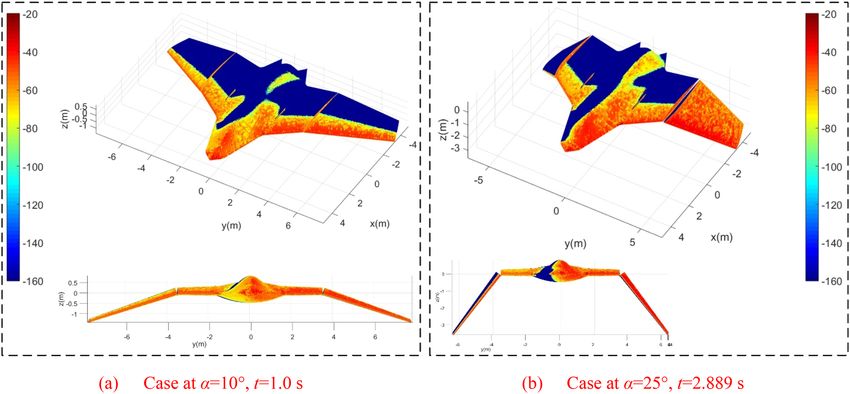
www.nature.com/scientificreports/

                                 outer wing 2, Mw1 is the grid coordinate matrix of mw1, Mw2 is the grid coordinate matrix of mw2, Mf is the grid
                                 coordinate matrix of mf.
                                    When each part of the wing begins to deform and the fuselage remains stationary in the coordinate system,
                                 the hybrid grid matrix of the aircraft could be transformed into:

                                                                                                                                              (2)

                                             M a (ma (t)) = M r1 (mr1 (t)), M r2 (mr2 (t)), M w1 (mw1 (t)), M w1 (mw2 (t)), M f (mf (t=0))

                                    At this time, the grid matrix of the aircraft is the combination of the static grid matrix of the fuselage and the
                                 dynamic grid matrix of each part of the wing.
                                    When the outer wing and the middle wing deflect together, the local hybrid matrix could be expressed as:

                                                                                                                                                   (3)

                                                                  M rw1 (mrw1 (t)) = M r1 (mr1 (t)), M w1 (mw1 (t))

                                 where mrw1 is a combined model of the mid wing 1 and the outer wing 1, Mrw1 is the grid coordinate matrix of
                                 mrw1.
                                    Then the hybrid matrix of the aircraft could be updated to:
                                                                          yx                yx
                                                                                                                                          (4)

                                                          M a (ma (t)) = M rw1 (mrw1 (t)), M rw2 (mrw2 (t)), M f (mf (t))

                                 where mrw2 is a combined model of the mid wing 2 and the outer wing 2, Mrw2 is the grid coordinate matrix of
                                 mrw2, different superscripts represent different transformation operations. The expression of this hybrid matrix
                                 is not unique, while the purpose is to integrate the outer wing and middle wing on the left and right sides of
                                 the aircraft.

                                 Matrix transformation during folding deformation. For the Z1 folding mode, when the outer wing 1
                                 deflects downward, its dynamic model could be expressed as:
                                                             y
                                                                                                                              (5)

                                                           M r1 (mr1 (t = 0)) = M r1 y(mr1 (t = 0)) − Yr1 |Am1 = 0

                                                                                               y
                                                              M zr1 (mr1 (t = 0)) = M r1 (z(mr1 (t = 0)) + Zr1 )|Am1 = 0                              (6)

                                                                              1     0            0


                                                    M xr1 (mr1 (t))   =       0 cos Ar1 (t) − sin Ar1 (t)       · M zr1 (mr1 (t   = 0))              (7)

                                                                              0 sin Ar1 (t) cos Ar1 (t)                                A
                                                                                                                                         m1   =0
                                 where Yr1 is the distance from the axis of rotation of the outer wing 1 around the middle wing 1 to the xz plane,
                                 Zr1 is the distance from the axis of rotation of the outer wing 1 around the middle wing 1 to the xy plane, different
                                 superscripts of Mr1 correspond to the current transformation operation. The wing here is regarded as a rigid body
                                 model, and the support on which it deflects is regarded as a rigid body and a stable fixed support. The deflection
                                 transformation operation of the outer wing 2 is similar to that of the outer wing 1. Return the transformed outer
                                 wing model to the outer end of the middle wing, thus the dynamic matrix of the aircraft could be expressed as:
                                                           yx               yx
                                                                                                                                                   (8)

                                          M a1 (ma1 (t)) = M r1 (mr1 (t)), M r2 (mr2 (t)), M w1 (mw1 (t = 0)), M w1 (mw2 (t = 0)), M f (mf (t=0))

                                 where ma1 represents the aircraft model in Z1 folding mode, Ma1 is the grid coordinate matrix of ma1.
                                   Under the irradiation of radar waves, the irradiation area on the surface of the aircraft could be extracted as:
                                                                                         Sa1 (t) ⇐ M a1 (ma1 (t))                                     (9)
                                 where Sa1 represents the irradiation area on the surface of the aircraft.
                                    For the Z2 folding mode, the middle wing and the outer wing deflect upward together. Then the middle wing
                                 1 and the outer wing 1 are combined into a whole:

                                                                                                                                         (10)

                                                           M rw1 (mrw1 (t = 0)) = M r1 (mr1 (t=0)), M w1 (mw1 (t = 0))

                                     The deflection process can be described as:
                                                                  y
                                                                                                                                                     (11)

                                                                M rw1 (mrw1 (t = 0)) = M rw1 y(mrw1 (t = 0)) − Yw1

                                                                                                    y
                                                                M zrw1 (mrw1 (t = 0)) = M rw1 (z(mrw1 (t = 0)) − Zw1 )                               (12)

                                                                                      1      0            0

                                                      M xrw1 (mrw1 (t))       =       0 cos Am1 (t) − sin Am1 (t)        · M zrw1 (mrw1 (t = 0))     (13)
                                                                                      0 sin Am1 (t) cos Am1 (t)
                                 where Yw1 is the distance from the axis of the mid wing 1 rotating around the fuselage to the zx plane, Zw1 is
                                 the distance from the axis of the mid wing 1 rotating around the fuselage to the xy plane. For the other half of
                                 the wing, the deflection transformation operation is similar to that of the outer wing 1 and the middle wing 1.
                                 Return the transformed wing model to the rotation axis on the side of the fuselage, and the dynamic matrix of
                                 the entire aircraft can be updated to:

Scientific Reports |   (2022) 12:4452 |               https://doi.org/10.1038/s41598-022-08385-9                                                        3

                                                                                                                                                   Vol.:(0123456789)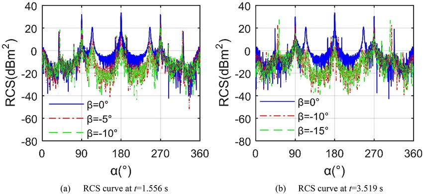
www.nature.com/scientificreports/
yx yx
(14)
M a2 (ma2 (t)) = M rw1 (mrw1 (t)), M rw2 (mrw2 (t)), M f (mf (t=0))
where ma2 is the aircraft model in Z2 folding mode, Ma2 is the grid coordinate matrix of ma2. Thus the irradiation
area on the surface of the aircraft can be extracted as:
Sa2 (t) ⇐ M a2 (ma2 (t)) (15)
where Sa2 represents the irradiation area on the surface of ma2.
For the Z3 folding mode, the mid wing 1 deflects upwards:
y
(16)
M w1 (mw1 (t = 0)) = M w1 y(mw1 (t = 0)) − Yw1
y
M zw1 (mw1 (t = 0)) = M w1 (z(mw1 (t = 0)) − Zw1 ) (17)
1 0 0
M xw1 (mw1 (t)) = 0 cos Am1 (t) − sin Am1 (t) · M zw1 (mw1 (t = 0)) (18)
0 sin Am1 (t) cos Am1 (t)
At the same time, the outer wing 1 follows the outer end of the mid wing 1 to translate:
y
(19)
M r1 (mr1 (t)) = M r1 y(mr1 (t = 0)) + �Yr1 (t)
y
M zr1 (mr1 (t)) = M r1 (z(mr1 (t)) + �Zr1 (t)) (20)
where ΔYr1 and ΔZr1 represent the translation distance of the outer wing 1 shaft in the y-axis and z-axis direc-
tions, respectively. Noting that:
�Yr1 (t)=Ym1 + R0 cos (Am1 (t) − A0 ) − Yr1 (21)
�Zr1 (t)=Zm1 + R0 sin (Am1 (t) − A0 ) − Zr1 (22)
where R0 is the distance between AX1 and AX2, AX1 represents the axis of rotation of the outer wing 1 around the
mid wing 1, AX2 is the axis of rotation of the mid wing 1 around the fuselage. A0 is the angle between the line
connecting the projection points of AX1 and AX2 on the yz plane and the xy plane in the initial state. Follow the
above steps to transform the mid wing 2 and the outer wing 2, and then perform the return operation, thus the
dynamic matrix of the aircraft can be updated to:
yz yz yx yx
(23)
M a3 (ma3 (t)) = M r1 (mr1 (t)), M r2 (mr2 (t)), M w1 (mw1 (t)), M w1 (mw2 (t)), M f (mf (t=0))
where ma3 is the aircraft model in Z3 folding mode, Ma3 is the grid coordinate matrix of ma3. The irradiation
area could be extracted as:
Sa3 (t) ⇐ M a3 (ma3 (t)) (24)
where Sa3 represents the irradiation area on the surface of ma3.
For the Z4 folding mode, the outer wing 1 translates with the mid wing 1 while also deflecting downwards:
y ′
(25)
M r1 (mr1 (t)) = M r1 y(mr1 (t = 0)) − Yr1 (t)
y
M zr1 (mr1 (t)) = M r1 z(mr1 (t)) + Zr1
′
(26)
(t)
1 0 0
M xr1 (mr1 (t)) = 0 cos Ar1 (t) − sin Ar1 (t) · M zr1 (mr1 (t)) (27)
0 sin Ar1 (t) cos Ar1 (t)
The relevant change parameters are updated as follows:
′
Yr1 (t)=Ym1 + R0 cos (Am1 (t) − A0 ) (28)
′
Zr1 (t)=Zm1 + R0 sin (Am1 (t) − A0 ) (29)
Zm1 + R0 sin (Am1 (t) − A0 ) + h0
Ar1 (t) = arcsin (30)
R1
where h0 is airfoil thickness at the root of outer wing 1, R1 is the length of outer wing 1. The matrix of the aircraft
and the illuminated area can be updated to:
xy xy yx yx
(31)
M a4 (ma4 (t)) = M r1 (mr1 (t)), M r2 (mr2 (t)), M w1 (mw1 (t)), M w1 (mw2 (t)), M f (mf (t=0))
Scientific Reports | (2022) 12:4452 | https://doi.org/10.1038/s41598-022-08385-9 4
Vol:.(1234567890)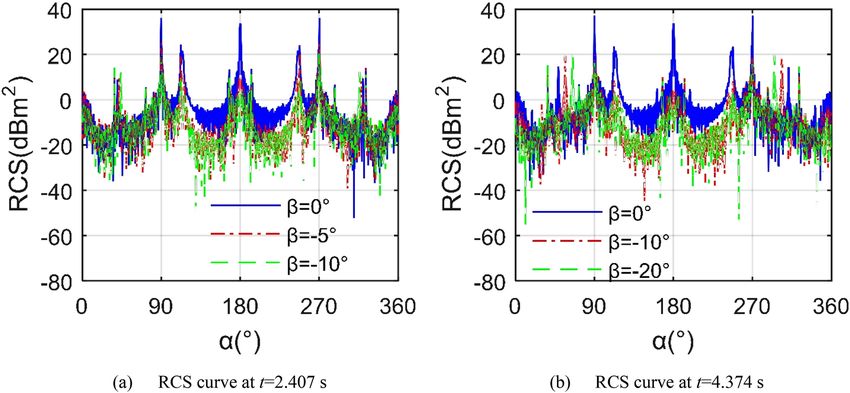
www.nature.com/scientificreports/
Sa4 (t) ⇐ M a4 (ma4 (t)) (32)
where ma4 is the aircraft model in Z4 folding mode, Ma4 is the grid coordinate matrix of ma4, where Sa4 represents
the irradiation area on the surface of ma4.
Electromagnetic scattering calculation. There are large areas of curved surfaces on the fuselage and
various parts of the wings, then PO method is used to solve the scattering contribution of the facets, where the
scattered electric field in the far field can be described as:
e−jkr
1
′ ′
Es(ma (t)) = J s e−jks·r dS+jks ρs e−jks·r dS
−jωµ
4πr ε ∀S(t) ∈ {Sa1 (t), Sa2 (t), Sa3 (t), Sa4 (t)}
S(t) S(t)
(33)
where k is the wave number in free space, μ is the magnetic permeability, ω is the angular frequency, Js is the
surface current, s means radiation direction, r is the field point, r′ is the source point coordinate vector, ε is the
dielectric constant, ρs is the charge density, dS is the integral facet.
For plane waves, the RCS contributed by the facets can be calculated as:
√ e s · E (m a (t))
s
(34)
σF (t) = lim 4πR2
R→∞ |E i |
where σ is the radar cross-section, subscript F represents the facet contribution, R is the distance between the
field point and the source point, Ei is the electric field intensity at the point of incidence, es is the direction of the
scattered electric field. Further transform the RCS calculation formula:
� √ 1 e −jkr � ′
σF (t) = 4πR2 −jωµ e s · J s e−jks·r dS (35)
|E i | 4πr
S(t)
Noting that the surface current could be expressed as:
2n × Hi , ZI
Js =
0 , ZD (36)
where n is the normal vector outside the surface element, ZI is the illuminated area, ZD is the unilluminated area,
Hi represents the magnetic field intensity of the incident point. Considering the relationship between electric
field and magnetic field, the facet RCS can be obtained as:
jk
σF (t) = √ n · (e s × hi )ejkw·r 0 I(t) (37)
π
where r0 is the coordinate vector of the reference point on the integral surface element, hi is the direction of
the incident magnetic field, i is the unit vector of the incident wave, I(t) is an integral expression, which can be
obtained according to the following calculation when the triangular facets are used:
w=s−i (38)
3 � � � �
ejkw·r m (t) � kw·Lm
p · Lm sinc , �p� �= 0
(39)
2 2
I(t) = jk|p| m=1 � �
Af , �p� = 0
where Lm is the vector of the m-th edge on the facet, Af is the area of the integral facet, noting that p is a defined
vector cross product:
sinc(x) = sin x/x (40)
p=n×w (41)
PTD is used to solve the edge diffraction contribution of the target, then the total RCS could be obtained as:
2
N
N
F (t)
E (t)
σ (t) = σF (t)
i
+ σE (t) , t ∈ [0, Tob ]
j (42)
i=1 j=1
where σE is the radar cross-section with the edge contribution. NF is the number of facets, NE is the number of
edges, and Tobs is the recommended length of time for observation, in order to ensure that the predetermined
deflection action is completed. For more descriptions of PO + PTD, please refer to the literature18,21.
To visually analyze and judge the scattering effect of the target surface, a custom surface scattering intensity
could be written as follows:
Scientific Reports | (2022) 12:4452 | https://doi.org/10.1038/s41598-022-08385-9 5
Vol.:(0123456789)
www.nature.com/scientificreports/
Figure 2. The Validation of HGMT on the outer wing 1, fRH = 6 GHz, β = 3°, ωr1 = 0.3142 rad/s.
σf (i) − σfn
Iss (i) = Kcd (Bcm − Bcn ) + Kcd · Bcn (43)
σfm − σfn
where Iss(i) is custom surface scattering intensity, σf represents the facet RCS under the current condition, the i in
brackets is the facet number, Kcd is the color depth control factor, σfn is the minimum of the facet RCS, σfm is the
maximum of the facet RCS, Bcm and Bcn represent the upper and lower boundaries of the current color window,
respectively. For more details on dynamic RCS, refer to r eference26.
Method verification. The Validation of HGMT method is presented in Fig. 2, where fRH represents to radar
wave frequency and horizontal polarization, ωr1 is deflection angular velocity of outer wing 1. For the RCS ~ t
curves, PO + MOM (method of moment)/MLFMM (multi-level fast multipole method) in FEKO (FEldberech-
nung bei Korpern mit beliebiger Oberflache) is used to calculate the RCS of the target, where QSP is used to
discretize the deflection state of outer wing 1. The mean RCS of HGMT curve is − 13.59 dBm2, while that of
discrete points obtained by FEKO is − 13.24 d Bm2. At t = 1.944 s, the outer wing 1 deflected down by 34.992°,
where the RCS of the HGMT curve is − 18.32 dBm2, that of the other curve is − 17.66 dBm2. It could be found
that the HGMT curve passes through the FEKO discrete points well, and different calculation methods lead to
the local and mean errors of RCS. In addition to the errors caused by different calculation methods, there are
also differences between the unstructured mesh generation used in this paper and the mesh generation used in
FEKO. In order to obtain the calculation model at different times, QSP needs to pay a lot of work and operation
steps. HGMT can continuously and conveniently handle RCS changes caused by wing deflection. These results
show that HGMT is feasible and accurate, and is used to calculate the electromagnetic scattering characteristics
of the wing during continuous deflection.
For the RCS ~ α curves, the downward deflection angle of the outer wing 1 is equal to 19.998°. It can be found
that the two RCS curves are roughly similar, including shape, peak position and number of peaks. The mean RCS
of the HGMT curve is − 8.39 d Bm2, that of the other is − 8.54 dBm2. When the azimuth angle is equal to 270°,
the RCS of HGMT is 13.03 d Bm2, and the RCS of FEKO is 12.33 d Bm2. For RCS ~ α curve and RCS ~ β curve,
the existing technologies including MOM and PO methods are feasible and widely used. Other obvious differ-
ences are reflected in the number of minima and individual maxima, because different calculation methods and
the difference in the number of curve base points will bring errors to the indicator. The current calculation state
is only an instantaneous state, and the different folding modes of the variant aircraft reflect complex dynamic
changes, which is obviously inconvenient to deal with by conventional methods. These results show that HGMT
is feasible and accurate to deal with the electromagnetic scattering characteristics of the target in transient state
and dynamic folding.
Model
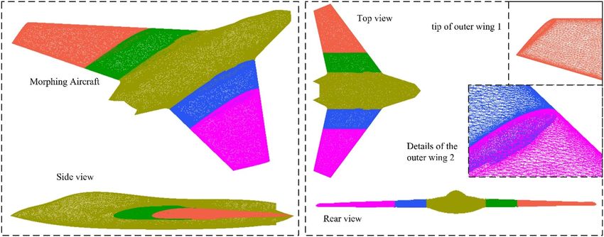
The model of the aircraft is built as shown in Fig. 3, where Rm is the length of mid wing 1, Lf is the length of
the aircraft fuselage, Ale is the sweep angle of the leading edge of the wing, Ate is the sweep angle of the trailing
edge of the wing, Wf is the wingspan of the aircraft, Atc is the cutting angle of the wing tip, Hf is the height of
the aircraft fuselage, Ans is the angle of the sideline of the nose, Wnz is the outer width of the nozzle, Ltc is the cut
length of the tail of the fuselage. According to the actual needs, the actual folding angle of the four modes can
be larger within the allowable range. When the rotation axis of the folding action is set at another appropriate
position, the folding mode will change.
The main size of the aircraft model is presented in Table 1, where this aircraft uses a symmetrical design,
which makes the outer wing 1 and outer wing 2 symmetrically distributed about the xz plane, and the mid wing
1 and mid wing 2 are symmetrical about the xz plane. The leading edge and trailing edge of the wing are designed
with a swept back, and the wing tip has been cut off.
Scientific Reports | (2022) 12:4452 | https://doi.org/10.1038/s41598-022-08385-9 6
Vol:.(1234567890)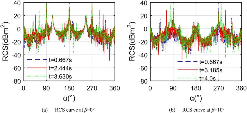
www.nature.com/scientificreports/

                                 Figure 3.  Aircraft model and main parameter distribution.

                                  Parameter   Lf (m)    Wf (m)   Ale (°)   Hf (m)    Ate (°)   Atc (°)
                                  Value       9.911     16       36.713    1.312     12.515    22.35
                                  Parameter   Ltc (m)   R1 (m)   Rm (m)    Ans (°)   h0 (m)    Wnz (m)
                                  Value       0.611     4.5      1.8       17.463    0.365     1.728

                                 Table 1.  The main size distribution of the aircraft model.

                                 Figure 4.  Detail display of outer wing 1 and mid wing 1.

                                     The details of the outer wing 1 are shown in Fig. 4, where the outer wing 1 and mid wing 1 are combined by
                                 AX1, and mid wing 1 and fuselage are combined by AX2. For the rotation axis AX1 and AX2 of the wing, the fairing
                                 is narrow and sharp as a whole, and the cross section is a combination of partial arcs and V shapes. Note that
                                 AX1 is set below the wing and AX2 is set above the wing. The V shape is placed on the surface of the wing and the
                                 arc is placed inside the plane.

Scientific Reports |   (2022) 12:4452 |                 https://doi.org/10.1038/s41598-022-08385-9                                              7

                                                                                                                                           Vol.:(0123456789)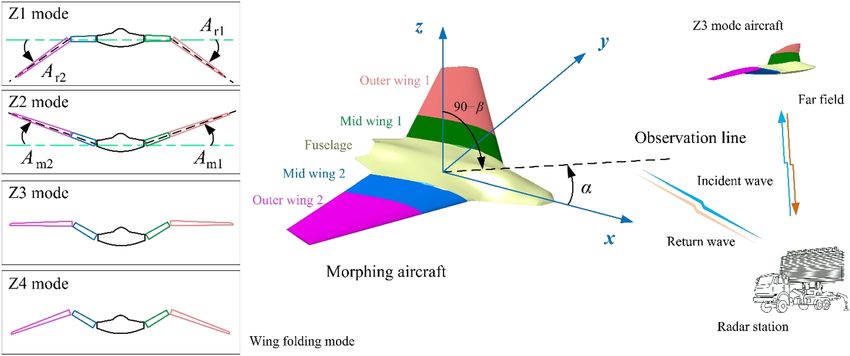
www.nature.com/scientificreports/
Figure 5. Meshing of the surface of each part of the aircraft.
Area Max size (mm) Area Max size (mm)
Global minimum size 1 Outer wing trailing edge 2
Outer wing leading edge 3 Wingtip curve 3
Mid wing leading edge 5 Mid wing trailing edge 5
Wing shaft surface 6 Nose curve 10
Edge of the fuselage 15 Tail line of fuselage 15
Wing end face 20 Outer wing surface 25
Mid wing surface 30 Fuselage surface 50
Table 2. The mesh size distribution on the surface of each part of the aircraft.
The surface of the fuselage and each section of the wing is processed with high-precision unstructured grid
technology as shown in Fig. 5, where the outer wing and the middle wing are not deflected in the initial state.
For the outer wing, the leading edge, trailing edge, wing tip, and rotating shaft of the wing are areas of smaller
size, where mesh density increase technology needs to be applied.
The mesh size distribution on the aircraft surface is provided in Table 2, where mesh density increase tech-
nology is widely used in curved surfaces with large changes in curvature or small area, including nose curve,
fuselage edge, nozzle, wing leading edge, wing tip, wing shaft and wing trailing edge. Note that each outer wing
has one shaft, and each mid wing has two shafts.
Results and discussion
Figure 6 presents that the increase of radar wave frequency brings obvious changes to the RCS ~ α and RCS ~ t
curves of outer wing 1. For the RCS ~ α curve, the outer wing 1 deflected downward by 33.336°, where the mean
value of the RCS curve under 6 GHz is equal to − 8.9423 d Bm2, that under 10 GHz is equal to − 8.2669 d Bm2.
It can be seen that the overall trend and peak value of these 3 RCS curves are similar, and there are many dif-
ferences in local fluctuations. For the RCS ~ t curve, the outer wing 1 continuously deflects downwards from a
horizontal position. There are obvious differences in the mean, local fluctuation and peak value of these three
RCS curves, where the peak of the RCS curve under 6 GHz is equal to 25.7755 dBm2, that under 8 GHz is equal
to 24.1351 d Bm2 as shown in Table 3. For the RCS curve at 10 GHz, it can be seen that the RCS value increases
with the increase of the deflection angle, and is accompanied by many violent jumps, because under the current
observation conditions, the angle between the illumination area on the upper surface of the outer wing 1 and
the radar wave gradually increases as the outer wing 1 continues to deflect downward. In this process, the strong
scattering source gradually shifts from the front surface to the upper surface. At an azimuth angle of 60°, the
average RCS index of the outer wing 1 generally decreases with the increase of the radar wave frequency. These
results indicate that the influence of the wing folding action on its radar stealth characteristics cannot be ignored.
Analysis of Z1 mode. Figure 7 supports that under current observation conditions, the Z1 mode will sig-
nificantly increase the strong scattering sources on the aircraft surface. For the case of α = 10° and t = 1.0 s, the
outer wing deflects downward by 18°, where the mid wing and fuselage are kept level. It can be found that the
nose, the top of the cockpit, the fusion of the wing fuselage and the leading edge of the wing have more red dis-
tribution. There is a small amount of yellow-green at the rear of the fuselage. When α = 25° and t = 2.889 s, the
increase in azimuth brings more red to the fusion of the nose, cockpit, and wing fuselage, while has less impact
Scientific Reports | (2022) 12:4452 | https://doi.org/10.1038/s41598-022-08385-9 8
Vol:.(1234567890)
www.nature.com/scientificreports/
Figure 6. RCS of the outer wing 1 under different radar wave frequencies, β = 0°, ωr1 = 0.3142 rad/s.
fRH (GHz) 2 4 6 8 10 12
Mean (dBm2) 5.5538 6.6450 5.4119 4.4112 2.0405 -0.4535
Peak (dBm2) 22.8069 25.8010 25.7755 24.1351 21.4936 17.5069
Table 3. RCS indicator of outer wing 1, α = 60°, β = 0°, ωr1 = 0.3142 rad/s, t = 0 ~ 3.857 s.
Figure 7. Surface scattering characteristics of aircraft in Z1 mode, β = 0°, fRH = 6 GHz, ωr1 = ωr2 = 0.3142 rad/s,
Am1 = Am2 = 0°, RCS unit: dBm2.
on the strong scattering source of the mid wing. At this time, the outer wing deflects 52.002° downward, where
the scattering enhancement effect brought by the folding action to the outer wing is very obvious, because both
the upper surface of the outer wing 1 and the lower surface of the outer wing 2 are completely illuminated by
radar waves. In addition, the gap between the outer wing and the middle wing is increased, and the scattering
intensity of the end face of the mid wing is also increased. These results show that the HGMT method is feasible
and intuitive to describe the electromagnetic scattering characteristics of the variant aircraft when the wings are
folded.
Figure 8 indicates that the dynamic RCS curve of the aircraft under different azimuth angles is quite different,
including the fluctuation range, peak size, peak number and change trend. For the RCS curve at α = 10°, the curve
has small fluctuations between − 12.97 and − 6.186 d Bm2, because the strong scattering sources on the aircraft
Scientific Reports | (2022) 12:4452 | https://doi.org/10.1038/s41598-022-08385-9 9
Vol.:(0123456789)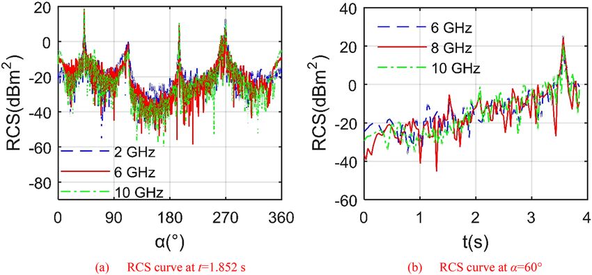
www.nature.com/scientificreports/
Figure 8. The influence of different azimuths on dynamic RCS of the aircraft in Z1 mode, β = 0°, fRH = 6 GHz,
ωr1 = ωr2 = 0.3142 rad/s, Am1 = Am2 = 0°.
Figure 9. RCS of the aircraft in Z1 mode, fRH = 6 GHz, ωr1 = ωr2 = 0.3142 rad/s, Am1 = Am2 = 0°.
surface are mainly concentrated on the fuselage head and the leading edge of the wing, and the deflection of the
outer wing has little effect on the illumination area. When α = 20°, the fluctuation range of the RCS curve has been
greatly increased, ranging from − 26.53 to − 3.521 d Bm2, which is mainly due to the scattering effect of the front
edge of the outer wing and its nearby curved surface. This increased volatility is also reflected in the RCS curve of
α = 30°, where the maximum value has reached 1.093 d Bm2. For the case of α = 50°, the fluctuating curve has an
obvious large peak, which is 23.85 dBm2 at 2.852 s, because the incident wave at this time is incident sideways, the
upper surface of the outer wing 1 becomes a dynamic scattering source. This prominent peak feature also exists
on the curves of α = 60° and α = 70°, where the maximum values are 17.88 d Bm2 and 32.32 d Bm2 respectively.
These results indicate that the azimuth angle has a greater impact on the dynamic RCS of the aircraft in the Z1
mode, and the RCS curve near the side fluctuates more obviously than the head.
Figure 9 reveals that at different instantaneous moments, the RCS ~ α curve of the aircraft will show obvious
differences, including the mean value and the local peak value. For the RCS curve at t = 0.667 s, the two largest
peaks appear in the lateral direction, 39.13 d Bm2 at α = 90.25° and 39.21 d
Bm2 at α = 270.3° respectively, where
the mean RCS of the curve is equal to 15.553 dBm2. When t = 2.444 s, the RCS curve has a peak of 21.58 dBm2 at
α = 46°, because the outer wing 1 deflected 43.992° downwards, the end face of the mid-section wing 1 is exposed,
and the upper surface of the outer wing 1 is also not conducive to deflecting radar waves to a non-threatening
direction. For the case of t = 3.630 s, the mean index of the RCS curve increased to 16.003 d Bm2, while the change
of the maximum peak is not obvious. When β = 10°, the peak and average levels of the RCS curve with t = 4.0 s
are significantly higher than the other two, where the mean of the RCS curve at t = 0.667 s is 7.373 d Bm2, that
at t = 3.185 s is 6.227 dBm2 as shown in Table 4. It is worth noting that increasing the elevation angle from 0° to
10° significantly reduces the average index of the RCS curve at t = 0.667 s. These results show that although the
Scientific Reports | (2022) 12:4452 | https://doi.org/10.1038/s41598-022-08385-9 10
Vol:.(1234567890)www.nature.com/scientificreports/
β = 0° β = 10°
t (s) 0.667 2.444 3.630 0.667 3.185 4.0
Mean (dBm2) 15.5527 15.7285 16.0027 7.3727 6.2272 12.8321
Peak (dBm2) 39.2094 39.7478 39.8298 32.1615 28.6215 37.9374
Table 4. RCS indicator of the aircraft in Z1 mode, α = 0° ~ 360°, fRH = 6 GHz, ωr1 = ωr2 = 0.3142 rad/s,
Am1 = Am2 = 0°.
Figure 10. RCS of the aircraft under different azimuths, β = 0°, fRH = 6 GHz, ωm1 = ωm2 = 0.1963 rad/s.
α (°) 10 20 30 80 90 100
Mean (dBm2) − 6.6604 − 13.5478 − 14.5690 − 5.6471 30.7186 − 0.0831
Peak (dBm2) − 1.9564 − 7.3101 − 6.2955 0.7757 45.8095 5.6211
Table 5. RCS indicator of the aircraft, β = 0°, fRH = 6 GHz, ωm1 = ωm2 = 0.1963 rad/s, t = 0 ~ 4.407 s.
aircraft in Z1 mode only deflects the outer wing, this folding action will bring a non-negligible change to the
stealth characteristics of the aircraft.
Analysis of Z2 mode. Figure 10 manifests that under the given head azimuth angle, the RCS curve in Z2
mode fluctuates more than in Z1 mode. When α = 10°, the minimum value of the RCS curve is as low as − 20.23
dBm2 at 2.444 s, and the maximum value is -1.956 d Bm2 at 4.148 s as shown in Table 5. For the case of α = 20°,
the minimum RCS is − 28.79 dBm while that of the RCS curve at α = 30° is − 35.16 dBm2. The main contribu-
2
tion of the increase in RCS fluctuations under heading azimuth is mainly from the dynamic deflection changes
of the leading edge of the entire wing. Compared with the Z1 mode, the outer end wing and the middle wing in
the Z2 mode deflect upward together. Consider the situation under lateral azimuth, the RCS curve when α = 80°
fluctuates sharply between − 18.18 and 0.7757 dBm2, where the mean index is only equal to − 5.65 d Bm2. For
the RCS curve at α = 90°, it can be clearly observed that the overall level of this curve is higher than the other
two, where the mean RCS of the curve at α = 90° is 30.7186 dBm2, that at α = 100° is -0.0831 dBm2, because when
the radar wave is incident from the positive side direction, the side of the fuselage, the tail nozzle baffle and the
cockpit curved surface will provide more strong scattering sources, while the wing tip surface, wing tip edge and
illuminated area curved surface of the entire wing will bring dynamic changes to the aircraft RCS.
Figure 11 shows that under the given observation conditions, the decrease of the elevation angle can signifi-
cantly reduce the average level of the aircraft RCS curve. When t = 1.556 s, the RCS curve under β = 0° shows 3
large peaks, 32.24 d Bm2 at α = 90.25°, 33.76 dBm2 at α = 179.8° and 32.34 d Bm2 at α = 269.8°, where the tail end
face of the fuselage and the trailing edge of the wing make the main contribution to the maximum tail peak. The
average index of the RCS curve with β = − 5° dropped rapidly to 2.42 d Bm2, while the average index of the RCS
curve with β = − 10° was as low as 0.31 d Bm2 as shown in Table 6, because the reduction of the elevation angle
can effectively improve the distribution of strong scattering sources on the upper surface of the fuselage and
near the nozzle. For the case of t = 3.519 s, the wing deflects upward by 39.579°, the average index of the RCS
curve with β = − 15° is slightly higher than that with β = − 10° by 0.1045 d Bm2. It is worth noting that when the
elevation angle is equal to − 10°, the mean RCS of t = 1.556 s is higher than the index of t = 3.519 s. These results
Scientific Reports | (2022) 12:4452 | https://doi.org/10.1038/s41598-022-08385-9 11
Vol.:(0123456789)www.nature.com/scientificreports/
Figure 11. RCS of the aircraft under different elevation angle, fRH = 6 GHz, ωm1 = ωm2 = 0.1963 rad/s.
t = 1.556 s t = 3.519 s
β (°) 0 −5 − 10 0 − 10 − 15
Mean (dBm2) 11.8451 2.4182 0.3109 11.5293 1.5218 1.6263
Peak (dBm2) 33.7636 24.9116 20.8882 33.7569 23.1870 27.7457
Table 6. RCS indicator of the aircraft, α = 0° ~ 360°, fRH = 6 GHz, ωm1 = ωm2 = 0.1963 rad/s.
Figure 12. Surface scattering characteristics of aircraft in Z3 mode, β = 5°, fRH = 6 GHz, ωm1 = ωm2 = 0.1963 rad/s,
Bm2.
RCS unit: d
show that the Z2 mode has a profound impact on the aircraft RCS, including dynamic amplitude, average value
and peak value.
Analysis of Z3 mode. Figure 12 presents that in the Z3 folding mode, the radar waves incident from the
side will cause more strong scattering sources on the surface of the aircraft than those from the head. When
α = 29° and t = 2.63 s, the mid wing deflects upwards by 29.58°, and the outer wing remains level. The nose, the
Scientific Reports | (2022) 12:4452 | https://doi.org/10.1038/s41598-022-08385-9 12
Vol:.(1234567890)www.nature.com/scientificreports/
Figure 13. RCS of the aircraft in Z3 mode under various azimuths, β = 0°, fRH = 6 GHz, ωm1 = ωm2 = 0.1963 rad/s.
α (°) 10 20 30 70 80 90
Mean (dBm2) − 6.5051 − 12.5186 − 18.4253 − 12.0001 − 5.0794 28.0423
Peak (dBm2) − 2.1126 − 7.6584 − 11.1492 − 5.1155 1.6669 43.0769
Table 7. RCS indicator of the aircraft, β = 0°, fRH = 6 GHz, ωm1 = ωm2 = 0.1963 rad/s, t = 0 ~ 4.407 s.
cockpit surface, the leading edge and outer end face of the mid wing 1, the leading edge of the outer wing 1, and
the upper surface of the mid wing 2 all show red and orange red. The surfaces near the trailing edge of outer wing
1 and outer wing 2 both show low-intensity scattering areas. For the case of α = 75°, t = 4.33 s, the orange-red in
the lighting area of the fuselage changed to red, and the original red was further deepened, which is mainly due
to the increase in the azimuth angle of the incident radar wave. The red range of the lower surface of the mid
wing 1 and the upper surface of the mid wing 2 is enlarged and deepened because of the combined effect of wing
deflection and azimuth angle change. In addition, the upper surface of the outer wing 1 is all lit, while the leading
edge of the outer wing 2 is transformed into a low scattering intensity area. The red color of the outer end face
of the mid-section wing 1 is deepened, and the red color of the inner end face of the outer wing 2 turns to dark
red. Due to the lateral offset of the azimuth angle, the orange and yellow colors in the low-scattering half of the
fuselage are further reduced. These results indicate that although the outer wing remains level, the strong scat-
tering source brought by the mid-section wing surface and the leading edge of the outer wing is still considerable
under current observation conditions.
Figure 13 provides that under the same azimuth, the dynamic RCS curve of the aircraft in Z3 mode is obvi-
ously different from the previous two modes. For the RCS curve at α = 10°, the minimum value is equal to -19.8
dBm2 which occurs at t = 2.963 s, where the mean RCS is − 6.5051 dBm2 as shown in Table 7. The fluctuation
range of the RCS curve of α = 20°is larger than that of the curve of α = 30°, while the average and minimum values
of the latter are smaller. When considering the side incident radar waves, the dynamic RCS curve of α = 90° is
still significantly higher than the other two curves, because at this time, the sides of the fuselage, the outer wing
tips and the cockpit will all provide strong scattering characteristics, while the continuous deflection of the mid-
section wing will continue to provide dynamic RCS changes. As the azimuth angle increases from 70° to 80°, the
RCS average index increases from – 12 to − 5.08 d Bm2, where the peak indicator received an increase of 6.7824
dBm2, because the curvature of the lower surface of the mid wing is generally small and the surface is smooth,
the increase in the azimuth angle will increase the angle between the radar wave and the lower surface of the mid
wing, which is not conducive to deflecting the incident wave. Compared with the Z2 mode, the aircraft in the Z3
mode has a slight decrease in the peak and average values of the RCS curve of 90° azimuth, while the peak and
average indicators of the RCS curve of the 80° azimuth are slightly increased.
Figure 14 shows that in the Z3 mode, the folding deformation of the wings brings significant changes to the
aircraft RCS ~ α curve, including the mean and the peak value. For the RCS curve at t = 2.407 s, the RCS curve
with β = 0° is significantly higher than the other two, where its average value is as high as 12.68 d
Bm2 as shown in
Table 8, because the outer end wing 1 and outer end wing 2 are always kept horizontal, making their outer ends
have a poor deflection effect on the incident side waves. When β = − 5°, the average RCS index is reduced to 4.59
dBm2, while the peak index is reduced by 9.6255 dBm2. As the elevation angle continues to decrease to -10°, the
peak value continues to decrease, with a magnitude of 20.69 dBm2 appearing at 269.8 azimuth. Considering the
RCS curve at t = 4.374 s, the mid wing deflects upwards by 49.1951°, and the outer wing remains level. As the
elevation angle decreases from 0° to − 10°, the mean indicator decreases by 12.441 dBm2. When the elevation
angle continues to decrease to -20, the change in peak value and average value appears small. These results show
Scientific Reports | (2022) 12:4452 | https://doi.org/10.1038/s41598-022-08385-9 13
Vol.:(0123456789)www.nature.com/scientificreports/
Figure 14. RCS of the aircraft in Z3 mode, fRH = 6 GHz, ωm1 = ωm2 = 0.1963 rad/s.
t = 2.407 s t = 4.374 s
β (°) 0 −5 − 10 0 − 10 − 20
Mean (dBm2) 12.6751 4.5932 − 0.0170 13.2345 0.7935 0.8152
Peak (dBm2) 36.2149 26.5894 20.6871 37.2017 20.3356 19.8817
Table 8. RCS indicator of the aircraft in Z3 mode, α = 0° ~ 360°, fRH = 6 GHz, ωm1 = ωm2 = 0.1963 rad/s.
Figure 15. RCS of the aircraft in Z4 mode under various azimuths, β = 0°, fRH = 6 GHz, ωm1 = ωm2 = 0.1963 rad/s.
that compared with the Z2 mode, the Z3 mode will bring some beneficial improvements to the average and peak
indicators of the RCS ~ α curve under the current observation conditions.
Analysis of Z4 mode. Figure 15 presents that as the azimuth angle of the incident wave approaches side-
ways, the average level of the aircraft dynamic RCS curve is increased. For the case of forward direction α = 30°,
the average RCS is as low as − 16.34 dBm2 as shown in Table 9, where the fluctuation range is − 28.62 to − 8.77
dBm2. When α = 50°, the fluctuation range of the RCS curve has been expanded, and the peak value has also
increased significantly. As the azimuth continues to increase to 70°, the average RCS increases to − 9.94 dBm2.
Consider the positive side incidence, it can be found that the average and peak levels of the RCS curve with
α = 90° are significantly higher than other curves, because at this time, the side of the fuselage, the cockpit, the
wingtip and the upper surface of the outer wing 1 can provide strong scattering sources. When α = 110°, the
average value of the RCS curve drops to 5.7538 d Bm2, and the fluctuation range is − 2.936 to 8.841 d
Bm2. Con-
sider the tail direction where α = 150°, the fluctuation range is reduced to − 5.844 to − 3.185 dBm2, because the
Scientific Reports | (2022) 12:4452 | https://doi.org/10.1038/s41598-022-08385-9 14
Vol:.(1234567890)www.nature.com/scientificreports/
α (°) 30 50 70 90 110 150
Mean (dBm2) − 16.3428 − 11.5747 − 9.9412 27.2634 5.7538 − 4.4090
Peak (dBm2) − 8.7727 2.5163 − 2.3069 40.8553 8.8411 − 3.1851
Table 9. RCS indicator of the aircraft, β = 0°, fRH = 6 GHz, ωm1 = ωm2 = 0.1963 rad/s, t = 0 ~ 4.407 s.
Figure 16. RCS of the aircraft in Z4 mode, fRH = 6 GHz, ωm1 = ωm2 = 0.1963 rad/s.
β = 0° β = − 10°
t (s) 1.3333 2.6296 3.6667 1.3333 3.3704 4.2593
Mean (dBm2) 11.6318 11.4199 11.6341 5.0710 1.5495 1.3879
Peak (dBm2) 33.7593 33.7582 33.7526 26.8809 21.0381 20.5785
Table 10. RCS indicator of the aircraft in Z4 mode, α = 0° ~ 360°, fRH = 6 GHz, ωm1 = ωm2 = 0.1963 rad/s.
dynamic scattering source in the tail direction at this time mainly comes from the trailing edge of the outer wing
and the mid wing, these areas all provide weak edge diffraction contribution. In general, compared with the Z3
mode, the average and peak indicators of the dynamic RCS curve of the aircraft under the 90° azimuth in the Z4
mode have been slightly reduced.
Figure 16 indicates that when the elevation angle is reduced from 0° to − 10°, the average and peak indica-
tors of the aircraft RCS in Z4 mode change more obviously. For the RCS curve at β = 0°, these three curves are
generally similar, while there are obvious differences locally, such as around 40.5 and 319.5 azimuths. When
t = 2.6296 s, the average value of the RCS curve is equal to 11.42 d Bm2 as shown in Table 10, and the peak value
is 33.76 dBm2. As time increases to 3.6667 s, the minimum value of the RCS curve has changed more, while the
average and peak indicators have changed less. These changes are mainly attributed to the fact that the sides and
the nose of the fuselage provide stable scattering sources for the incident radar waves in the horizontal plane,
while the leading and trailing edges of the wing contribute low dynamic scattering, the angle between the wing
surface and the horizontal plane is small, which makes the dynamic contribution of the facet weaker. Consider-
ing the case of β = − 10°, the tail performance of the three RCS curves is significantly reduced. The mean RCS
of the curve at t = 1.333 s is 5.071 d Bm2 at α = 296.8°. When the time is increased to
Bm2, and the peak is 26.88 d
3.3704 s, the average and peak value have been effectively reduced. As the mid wing and outer wing continue
to deflect, the average and peak values of the RCS curve can still maintain a low level, as can be seen in the case
of t = 4.2593 s. These results indicate that the aircraft deformation in Z4 mode can still maintain a low level of
scattering at an elevation angle of − 10°.
Conclusion
Based on the presented HGMT method, the electromagnetic scattering characteristics of the morphing aircraft in
the four Z-folding modes are studied and discussed. Through these investigations and analyses, this manuscript
can draw the following three conclusions (Supplementary information S1):
Scientific Reports | (2022) 12:4452 | https://doi.org/10.1038/s41598-022-08385-9 15
Vol.:(0123456789)www.nature.com/scientificreports/
(1) For a given incident wave, the deflection of the outer wing alone will bring significant dynamic changes to
its RCS, while in Z1 and Z2 folding modes, the maximum peak of the dynamic RCS of the aircraft under
the lateral azimuth is significantly higher than that under the head azimuth.
(2) Under the condition of positive lateral incident wave, the given folding deformation of the wing in Z3 mode
can significantly reduce the dynamic RCS level of the aircraft, where the fluctuation range of the RCS curve
after the maximum peak also appears relatively stable, while the maximum peak is reduced compared with
Z2 mode.
(3) In Z4 mode, the maximum peak of the dynamic RCS curve of the aircraft under the positive lateral azi-
muth is further reduced, where at the given negative elevation angle, the aircraft can still gain good stealth
characteristics, while the dynamic range of the RCS after the maximum peak becomes larger compared
with other modes.
Received: 4 November 2021; Accepted: 7 March 2022
References
1. Ajaj, R. M., Parancheerivilakkathil, M. S., Amoozgar, M., Friswell, M. I. & Cantwell W. J. Recent developments in the aeroelasticity
of morphing aircraft. Prog. Aerosp. Sci. 120, 100682 (2021)
2. Murfitt, S. L. et al. Applications of unmanned aerial vehicles in intertidal reef monitoring. Sci. Rep. 7(1), 1–11 (2017).
3. Chen, X. Y., Li, C. N. & Gong, C. L. A study of morphing aircraft on morphing rules along trajectory. Chin. J. Aeronaut. https://
doi.org/10.1016/j.cja.2020.04.032 (2020).
4. Chen, Q., Bai, P., Yin, W. L., Leng, J. S. & Li, F. Design and analysis of a variable-sweep morphing aircraft with outboard wing
section large-scale shearing. Acta Aerodyn. Sin. 31(1), 40–46 (2013).
5. Yue, T., Zhang, X. & Wang, L. Flight dynamic modeling and control for a telescopic wing morphing aircraft via asymmetric wing
morphing. Aerosp. Sci. Technol. 70, 328–338 (2017).
6. Ajaj, R. M., Beaverstock, C. S. & Friswell, M. I. Morphing aircraft: the need for a new design philosophy. Aerosp. Sci. Technol. 49,
154–166 (2016).
7. Lozano, F. & Paniagua, G. Airfoil leading edge blowing to control bow shock waves. Sci. Rep. 10(1), 1–18 (2020).
8. Zhan, P., Cheng, Y. & Mao, J. Research development of morphing aircraft in United States. New Viewpoint 12, 54–56 (2010).
9. Cheng, H. Y., Dong, C. Y. & Jiang, W. L. Non-fragile switched H∞ control for morphing aircraft with asynchronous switching.
Chin. J. Aeronaut. 30, 1127–1139 (2017).
10. Han, J. S. & Han, J. H. A contralateral wing stabilizes a hovering hawkmoth under a lateral gust. Sci. Rep. 9(1), 1–13 (2019).
11. Bubert, E. A., Woods, B. K. S. & Lee, K. Design and fabrication of a passive 1D morphing aircraft skin. J. Intell. Mater. Syst. Struct.
21, 1699–1717 (2010).
12. Guo, Q., Zhang, L., Chang, X. & He, X. Numerical simulation of dynamic aerodynamic characteristics of a morphing aircraft. Acta
Aerodyn. Sin. 29, 744–750 (2011).
13. Xu, D., Hui, Z. & Liu, Y. Morphing control of a new bionic morphing UAV with deep reinforcement learning. Aerosp. Sci. Technol.
92, 232–243 (2019).
14. Cheng, X. & Sun, M. Wing-kinematics measurement and aerodynamics in a small insect in hovering flight. Sci. Rep. 6, 25706
(2016).
15. Wen, N., Liu, Z. & Sun, Y. Design of LPV-based sliding mode controller with finite time convergence for a morphing aircraft. Int.
J. Aerosp. Eng. 2017, 8426348 (2017).
16. Chen, Q., Bai, P., Chen, N. & Li, F. Investigation on the unsteady aerodynamic characteristics of sliding-skin variable-sweep mor-
phing unmanned aerial vehicle. Acta Aerodyn. Sin. 29, 645–650 (2010).
17. Olympio, K. R. & Gandhi, F. Flexible skins for morphing aircraft using cellular honeycomb cores. J. Intell. Mater. Syst. Struct. 21,
1719–1735 (2010).
18. Zhou, Z. & Huang, JWu. Acoustic and radar integrated stealth design for ducted tail rotor based on comprehensive optimization
method. Aerosp. Sci. Technol. 92, 244–257 (2019).
19. Wu, M., Xiao, T. & Ang, H. Optimal flight planning for a Z-shaped morphing-wing solar-powered unmanned aerial vehicle. J.
Guid. Control. Dyn. 41, 497–505 (2018).
20. Wu, Z., Lu, J. & Zhou, Q. Modified adaptive neural dynamic surface control for morphing aircraft with input and output constraints.
Nonlinear Dyn. 87, 2367–2383 (2017).
21. Zhou, Z. Y. & Huang, J. Joint improvements of radar/infrared stealth for exhaust system of unmanned aircraft based on sorting
factor Pareto solution. Sci. Rep. 11(1), 1–16 (2021).
22. Chen, Q., Bai, P., Chen, N. & Li, F. Morphing aircraft wing variable-sweep: two practical methods and their aerodynamic charac-
teristics. Acta Aerodyn. Sin. 30, 658–663 (2012).
23. Zhu, H. J., Meng, X. G. & Sun, M. Forward flight stability in a drone-fly. Sci. Rep. 10(1), 1975 (2020).
24. Borcea, L., Druskin, V. & Zimmerling, J. A reduced order model approach to inverse scattering in lossy layered media. J. Sci.
Comput. 89(1), 1. https://doi.org/10.1007/s10915-021-01616-7 (2021).
25. Wang, P., Zheng, X., Yin, C. & Guo, S. Wing folding mechanism design and angle measurement for morphing aircraft. Adv. Aero-
naut. Sci. Eng. 4, 333–338 (2013).
26. Zhou, Z., Huang, J. & Wang, J. Compound helicopter multi-rotor dynamic radar cross section response analysis. Aerosp. Sci.
Technol. 105, 106047 (2020).
27. Wang, Q., Gong, L. & Dong, C. Morphing aircraft control based on switched nonlinear systems and adaptive dynamic program-
ming. Aerosp. Sci. Technol. 93, 105325 (2019).
28. Ahmed, A. S. & Ramanujan, R. V. Magnetic field triggered multicycle damage sensing and self healing. Sci. Rep. 5(1), 1–10 (2015).
29. Mirkovic, D. et al. Electromagnetic model reliably predicts radar scattering characteristics of airborne organisms. Sci. Rep. 6, 35637
(2016).
Acknowledgements
Thanks to Professor Jun Huang for guiding this work.
Scientific Reports | (2022) 12:4452 | https://doi.org/10.1038/s41598-022-08385-9 16
Vol:.(1234567890)www.nature.com/scientificreports/
Author contributions
Z.Z. and J.H. conceived the concept and method of the paper. Z.Z. designed the study and carried out the com-
putation; Z.Z. and J.H. analyzed the data. Z.Z. wrote the main manuscript text and prepared figures. Z.Z. and
J.H. checked the paper. All authors reviewed the manuscript.
Funding
This work was supported by the Project funded by China Postdoctoral Science Foundation (Grant Nos.
BX20200035, 2020M680005), and the National Natural Science Foundation of China.
Competing interests
The authors declare no competing interests.
Additional information
Supplementary Information The online version contains supplementary material available at https://doi.org/
10.1038/s41598-022-08385-9.
Correspondence and requests for materials should be addressed to Z.Z.
Reprints and permissions information is available at www.nature.com/reprints.
Publisher’s note Springer Nature remains neutral with regard to jurisdictional claims in published maps and
institutional affiliations.
Open Access This article is licensed under a Creative Commons Attribution 4.0 International
License, which permits use, sharing, adaptation, distribution and reproduction in any medium or
format, as long as you give appropriate credit to the original author(s) and the source, provide a link to the
Creative Commons licence, and indicate if changes were made. The images or other third party material in this
article are included in the article’s Creative Commons licence, unless indicated otherwise in a credit line to the
material. If material is not included in the article’s Creative Commons licence and your intended use is not
permitted by statutory regulation or exceeds the permitted use, you will need to obtain permission directly from
the copyright holder. To view a copy of this licence, visit http://creativecommons.org/licenses/by/4.0/.
© The Author(s) 2022
Scientific Reports | (2022) 12:4452 | https://doi.org/10.1038/s41598-022-08385-9 17
Vol.:(0123456789)You can also read