3D Geophysical Post-Inversion Feature Extraction for Mineral Exploration through Fast-ICA
←
→
Page content transcription
If your browser does not render page correctly, please read the page content below
minerals
Article
3D Geophysical Post-Inversion Feature Extraction for Mineral
Exploration through Fast-ICA
Bahman Abbassi *                 and Li-Zhen Cheng

                                          Institut de Recherche en Mines et en Environnement (IRME), Université du Québec en
                                          Abitibi-Témiscamingue (UQAT), Rouyn-Noranda, QC J9X 5E4, Canada; LiZhen.Cheng@uqat.ca
                                          * Correspondence: bahman.abbassi@uqat.ca

                                          Abstract: A major problem in the post-inversion geophysical interpretation is the extraction of geo-
                                          logical information from inverted physical property models, which do not necessarily represent all
                                          underlying geological features. No matter how accurate the inversions are, each inverted physical
                                          property model is sensitive to limited aspects of subsurface geology and is insensitive to other
                                          geological features that are otherwise detectable with complementary physical property models.
                                          Therefore, specific parts of the geological model can be reconstructed from different physical property
                                          models. To show how this reconstruction works, we simulated a complex geological system that
                                          comprised an original layered Earth model that has passed several geological deformations and
                                          alteration overprints. Linear combination of complex geological features comprised three physical
                                          property distributions: electrical resistivity, induced polarization chargeability, and magnetic suscep-
                                          tibility models. This study proposes a multivariate feature extraction approach to extract information
                                          about the underlying geological features comprising the bulk physical properties. We evaluated
                                          our method in numerical simulations and compared three feature extraction algorithms to see the
                                tolerance of each method to the geological artifacts and noises. We show that the fast-independent

                                          component analysis (Fast-ICA) algorithm by negentropy maximization is a robust method in the geo-
Citation: Abbassi, B.; Cheng, L.-Z.
                                          logical feature extraction that can handle the added unknown geological noises. The post-inversion
3D Geophysical Post-Inversion
                                          physical properties were also used to reconstruct the underlying geological sources. We show that
Feature Extraction for Mineral
                                          the sharpness of the inverted images is an important constraint on the feature extraction process.
Exploration through Fast-ICA.
Minerals 2021, 11, 959. https://
                                          Our method successfully separates geological features in multiple 3D physical property models.
doi.org/10.3390/min11090959               This methodology is reproducible for any number of lithologies and physical property combinations
                                          and can recover the latent geological features, including the background geological patterns from
Academic Editor: Michał Malinowski        overprints of chemical alteration.

Received: 31 July 2021                    Keywords: feature extraction; independent component analysis; 3D inversion; physical properties
Accepted: 30 August 2021
Published: 1 September 2021

Publisher’s Note: MDPI stays neutral      1. Introduction
with regard to jurisdictional claims in
                                               Integrated imaging methods provide a high potential for precise detection and char-
published maps and institutional affil-
                                          acterization of mineral deposits [1]. However, identifying distinct geological features is
iations.
                                          often very difficult and usually demands a detailed knowledge of prior petrophysical
                                          information, which is a piece of costly information during the early stages of an exploration
                                          program [1]. Therefore, inferring geological information from multiple physical property
                                          models without incorporating prior information adds value to pre-drilling decision-making
Copyright: © 2021 by the authors.
                                          assessments [1–6]. Nonetheless, the complex and irregular structures of the mineral de-
Licensee MDPI, Basel, Switzerland.
                                          posits lead to difficulties in the conventional 3D imaging methods. The overlap of physical
This article is an open access article
                                          properties between different rock units is a common characteristic of mineralization sys-
distributed under the terms and
                                          tems, and in most cases, additional chemical alteration heterogeneously overprints the
conditions of the Creative Commons
                                          whole system and eventually changes the bulk physical properties of rocks [1,2].
Attribution (CC BY) license (https://
                                               The current numerical advances are focused mainly on the inversion methodologies to
creativecommons.org/licenses/by/
4.0/).
                                          tackle the problem of non-uniqueness of the recovered physical properties through various

Minerals 2021, 11, 959. https://doi.org/10.3390/min11090959                                             https://www.mdpi.com/journal/minerals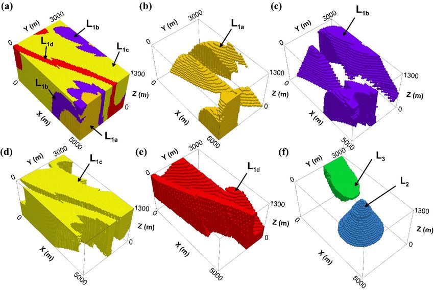
Minerals 2021, 11, 959                                                                                            2 of 20

                         methods such as borehole constrained inversion [3–6], cooperative inversion [7,8], and joint
                         inversion methods [9–13]. Though it is essential to recover accurate 3D physical property
                         models, a more fundamental phenomenon has remained untouched: the interdependency
                         of physical properties and their relation to the underlying geological factors. The question
                         is how efficiently one can reduce the effect of the physical properties’ overlap in the
                         underlying complex multicomponent geological systems, to uncover the hidden geological
                         features from multiple interdependent geophysical images.
                              This study explores a 3D implementation of independent component analysis (ICA)
                         to extract the underlying 3D geological features hidden inside multiple layers of 3D
                         geophysical images. The ICA algorithm in this study incorporates higher-order statistics to
                         separate a set of modeled images (physical properties) into the independent components
                         (geological features) without the need for further preliminary information.
                              ICA is an active and interdisciplinary research topic [14–17] with numerous applica-
                         tions in research areas such as remote sensing [18–21], medical imaging [22–24], and image
                         processing [25,26]. In geophysical research, the applications are mainly dedicated to the
                         exploration of seismology to handle the multidimensionality of seismic data and reduce
                         the unwanted seismic artifacts from raw data [27] or extract useful frequency features from
                         processed seismic data [28]. Therefore, the applications of ICA in geophysics are mostly
                         data-based, rather than model-based, implementations.
                              In this work, we used a 3D model-based implementation of ICA, or post-inversion
                         ICA, in which we viewed the lithological interpretation of inverted geophysical images
                         as a blind source separation problem. We propose an unmixing scheme that is based
                         on kurtosis and negentropy maximization principles. Our model-based ICA assumes
                         several underlying factors are responsible for the outputs of physical properties in each 3D
                         voxel cell. For example, the results of 3D inversion of three geophysical methods can be
                         expressed as three cell-based physical property models. These three models have some
                         correlations and dependencies that permeate the latent information from one space into
                         another. The ICA helps reduce the effect of this information leakage and lets each 3D
                         model characterize a unique representation of its underlying patterns that otherwise are
                         buried within large sets of model parameters. Our ICA algorithm statistically separates the
                         physical properties of rocks into independent components that are optimal approximations
                         of the hidden geological features. This study shows how the proposed feature extraction
                         scheme increases the accuracy of 3D geological interpretations, and how inversion artifacts
                         influence the robustness of the feature extraction procedure.
                              First, we simulated the interdependency between physical properties, including
                         magnetic susceptibility (χ), electrical resistivity (ρ), and induced polarization chargeability
                         (m) due to varying sensitivities of geophysical methods to the source geological features.
                         Then, we maximized the non-Gaussianity of inverted geophysical images through different
                         high-order statistical methods to recover the hidden geological features responsible for
                         the physical properties. Finally, we evaluated the geological information loss due to the
                         inversion of surface geophysical responses.

                         2. Materials and Methods
                         2.1. Theoretical Background
                              Geologists define specific assemblages of minerals as different lithotypes to differ-
                         entiate rocks in different macroscopic scales. However, geophysicists need to interpret
                         geophysical signals to recover physical property distributions that are usually linked to
                         the underlying geological patterns. Each physical property highlights different geological
                         features and can be mapped by relevant geophysical methods. This section demonstrates a
                         methodology to simulate the conversion of information from underground lithologies to
                         physical properties and then to the measured geophysical signals on the surface. Then, we
                         explain a reverse procedure to model these signals and recover an approximated image of
                         the physical properties. Then, we use a source separation method to retrieve the underlying
                         geological features from the modeled physical properties.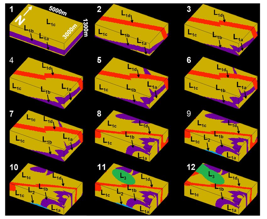
Minerals 2021, 11, 959                                                                                               3 of 20

                             A linear non-Gaussian mixing model was used in this study to create physical property
                         images (Pj ) from non-Gaussian independent lithological data (Li ) with an additional non-
                         Gaussian geological noise (PNoise ) as follows:

                                                              Pj =   ∑ aij Li + PNoise                                  (1)

                         where i = 1, 2, . . . , n denotes the number of the latent variables (geological features) and
                         j = 1, 2, . . . , m denotes the number of physical properties, and aij are the mixing weights.
                         For simplicity, we used a mixing model where m = n. A three-component model (n = m = 3)
                         was used for the mixing process in this study. When there is a one-to-one relationship
                         between physical properties and the underlying lithotypes, aij appears as an identity
                         matrix. In this simple case, we can easily interpret geophysical models mapping exact
                         geological features. However, the mixing process often has complicated forms since each
                         geophysical method is sensitive to one or more aspects of hidden geological factors. This
                         linear mixing petrophysical model helps us to simulate the overlap of physical properties
                         for different geological features. Depending on the sensitivity of each physical property
                         model (P1 , P2 , P3 ), different combinations of geological features (L1 , L2 , L3 ) comprise the
                         3D bulk physical property models. The problem is to find a separation matrix (wij ) that
                         tends to unmix the physical properties (Pj ) to recover the source geological features (Li ).
                               Equation (2) is the general formulation of a feature extraction process that eliminates or at
                         least reduces the effect of physical property overlaps. This has crucial importance in exploring
                         mineral targets with complex hydrothermal alteration patterns overprinted on background
                         geology. Efficient estimation of the separation matrix enables us to separate different geological
                         features, such as host rocks, from different episodes of hydrothermal alterations.

                                                                    Li =   ∑ wij Pj                                     (2)

                         2.2. Simulation of Exploration Procedure
                               A schematic workflow of a typical exploration procedure is presented in Figure 1a to
                         demonstrate the effect of 3D Earth on geological feature extraction during an exploration
                         program. Minerals comprise macroscopic geological features (L), and a petrophysical
                         system links physical properties (P) to the underlying geological features. The physical
                         properties appear on the Earth’s surface as geophysical signals (S) observed in the form of
                         magnetic and electrical potential fields. The imaging system aims to recover approximated
                         physical property models (P*) from observed signals to be interpreted in the feature
                         extraction system for retrieving an approximation of the latent lithotypes (Li *). Physical
                         properties and lithotypes marked with an asterisk (Pj * and Li *) indicate that they are
                         approximations of the underlying physical properties and lithological variations.
                               The proposed feature extraction procedure enables us to simulate the interpretation
                         system for quantitative geological feature extraction. We simulated an exploration system to
                         test our source separation methodology. Figure 1b represents a simulation of the exploration
                         process that is used throughout this study. The linear mixing system (petrophysical
                         system in Equation (1) creates physical properties (Pj ) from linear mixtures of the hidden
                         lithological factors (Li ). The simulation of the geophysical system consists of a well-posed
                         set of equations that calculates the geophysical responses (Sc ) of the 3D physical property
                         distributions on the Earth surface (forward modeling).

                                                                     Sc = f (Pj )                                       (3)

                         where f represents a forward problem operator that simulates the target geophysical
                         responses (signals), and c = 1, 2, 3, . . . , p denotes the number of p data points. Through
Minerals 2021, 11, 959 4 of 20
this, we simulated the synthetic field data (Sd ) to be fed into the imaging system with an
added non-Gaussian geophysical noise (SNoise ).
Minerals 2021, 11, x FOR PEER REVIEW Sd = Sc + SNoise (4)
where d = c.
Figure
Figure 1. 1. Workflow
Workflow of geological
of geological featurefeature extraction:
extraction: (a) An exploration
(a) An exploration system: The system: The syne
synergy of
hidden
the hiddenmixing petrophysical
mixing petrophysical system
system with with the geophysical
the geophysical system
system creates creates
observed observed geoph
geophysical
nals (S)
signals thatproduce
(S) that produce measured
measured physicalphysical properties
properties (P). The approximated
(P). The approximated physical propertiesphysical
(P*) prop
are used in a feature extraction system to recover the hidden geological factors (L).
are used in a feature extraction system to recover the hidden geological factors (L). (b) A s(b) A simulation of
the
of exploration system: Synthetic
the exploration system: geophysical
Synthetic signals (Sd ) are calculated
geophysical signals (Sfrom the forward
d) are responses
calculated from the fo
ofsponses
the simulated physical properties
of the simulated physical (P j ) that are linear mixtures of hidden geological
properties (Pj) that are linear mixtures of hidden features (Li ). geolo
Multiple inversions calculate the estimated physical properties (Pj *) that are used in the subsequent
tures (Li). Multiple inversions calculate the estimated physical properties (Pj*) that are u
feature extractions to retrieve an approximation of the latent lithotypes (Li *).
subsequent feature extractions to retrieve an approximation of the latent lithotypes (Li ). *
We inserted two sources of noise: geological and geophysical non-Gaussian noises.
The noises
The added proposed feature
helped extraction
us to compare the procedure
sensitivity ofenables
differentusfeature
to simulate the interp
extraction
methods to the unknown sources of outliers. We used a finite element
system for quantitative geological feature extraction. We simulated an exploratiomethod on the
three physical property models to calculate their apparent resistivity, chargeability, and
to test our source separation methodology. Figure 1b represents a simulation of th
total magnetic field responses [29–31]. In the case of the DC/IP forward problem, the
ration
IP processmodel
chargeability that is
is used throughout
considered as a smallthis study. The
perturbation oflinear mixingelectrical
the reference system (petro
system in Equation
conductivity (1) Normalized
model [30,32]. creates physical properties
chargeability (0 ≤ m(P≤j)1)from
tendslinear mixtures
to decrease the of th
reference conductivity (σ
lithological factors (LDC ) in the modeled IP phenomenon and produces a perturbed
i). The simulation of the geophysical system consists of a we
subsurface conductivity (σIP ) in the function
set of equations that calculates of [32] as follows:
the geophysical responses (Sc) of the 3D physical
distributions on the Earth surface
σIP = (forward
(1 − m)σDCmodeling). (5)
Sc = f(Ppotential
The program calculates the forward j) responses of two conductivity models
(σDC & σIP ) separately. The forward modeling σDC gives the apparent conductivity values
where f represents a forward problem operator that simulates the target geo
responses (signals), and c = 1, 2, 3, …, p denotes the number of p data points. Thro
we simulated the synthetic field data (Sd) to be fed into the imaging system with a
non-Gaussian geophysical noise (SNoise).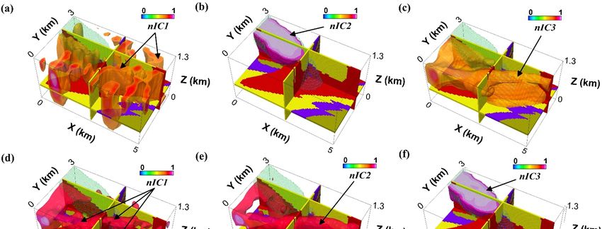
Minerals 2021, 11, 959                                                                                          5 of 20

                         (σa ), and the modeled potentials (φ) are used to calculate the apparent chargeabilities
                         based on [32].
                                                    m a = [φ(σIP ) − φ(σDC )]/φ(σDC )                         (6)
                              The imaging system approximates the physical properties (Pj *) through inverse mod-
                         eling as follows:
                                                            Pj∗ = f −1 (Sd )                                  (7)

                         where f −1 is the inverse problem operator. The recovered physical properties are then
                         used to reconstruct the hidden geological factors (Li *) through the higher-order statistical
                         unmixing process (Equation (2)).
                               In this study, we explore the effect of the smoothness and sharpness of the imaging
                         system on the output of the feature extraction system. This gives us a valuable view of
                         the way the sharpness of the imaging system could influence the recovered geological
                         features and provides means to predict how much information is essentially extractable
                         from geophysical imaging, i.e., to determine which parts of the spatial domain of the
                         original geology are vulnerable to the information loss due to the geophysical imaging.
                               We explore the two endpoints of the imaging scenarios (sharp versus smooth) in
                         DC/IP and magnetic inversions. We used a blocky inversion method for the inversion of
                         electrical resistivity and chargeability data [31,33,34] and an iterative reweighting inver-
                         sion [35,36] for inverse modeling of the magnetic susceptibility data. In each iteration of
                         DC/IP inversion, an incomplete Gauss-Newton least-squares optimization tries to reduce
                         the gap between measured and calculated properties (σa and m a ) by modifying the σDC
                         and σIP values. When the calculation reaches its threshold, the modeled resistivities and
                         chargeabilities are determined by ρ = 1/σDC and m = [1 − (σIP /σDC )], respectively.
                               The blocky inversion algorithm [34], which uses an extension of l2 -norm and l1 -norm
                         inversions, incorporates two cut-off factors in the DC/IP inversion—a data constraint
                         cut-off factor (0 < k1 < 1), and a model constraint cut-off factor (0 < k2 < 1). Large enough
                         cut-off factors result in smooth physical property models equivalent to l2 -norm results. The
                         iterative reweighting magnetic inversion takes the first iteration susceptibility and uses
                         it as an iterative reweighting constraint when running a new inversion. This process is
                         iterated until a satisfactory model is achieved [35,36]. Reweighting magnetic inversion
                         tends to recover sharp magnetic variations, and its results are equivalent to the robust or
                         blocky inversion in the DC/IP inversion [33,34].

                         2.3. Independent Component Analysis (ICA)
                              Traditional visualization techniques incorporating conventional gridding, slicing, and
                         clipping methods cannot identify subtle structures inside the high-dimensional geophysi-
                         cal images. In the presence of statistical correlation and independence, multivariate tools
                         are necessary to recover the hidden patterns inside multiple interdependent geophysical
                         images. Statistical measures provide collective clues about the behaviors of multivariate
                         spaces. Instead of treating every geophysical image separately, one can extract the un-
                         derlying features by making few general assumptions about the multivariate statistical
                         measures. The mixing process has three statistical characteristics [37] that need to be
                         considered to reconstruct an integrated geological model from physical properties. Firstly,
                         the source geological features are statistically uncorrelated and independent, while the
                         physical properties are correlated and interdependent due to the linear mixing process.
                         Secondly, the mixing process increases the normality or Gaussianity of the images, i.e., the
                         observed (or modeled) physical property images are more Gaussian than the underlying
                         lithological distributions. This results from the central limit theorem (CLT) in probability
                         theory that says the distribution of a sum of independent random variables tends toward
                         a Gaussian distribution. Later, we used this principle to maximize the non-Gaussianity
                         of physical properties using kurtosis maximization as a criterion for estimating hidden
                         geological features. Thirdly, the spatial complexities of the physical property images are
                         equal to or greater than that of the least complex geological feature distribution. We later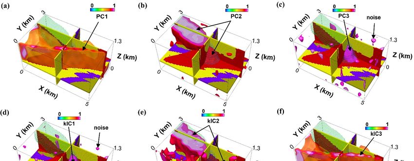
Minerals 2021, 11, 959                                                                                          6 of 20

                         used this general principle to maximize the non-Gaussianity of physical properties using
                         negentropy maximization as a criterion for estimating hidden geological features.
                                One crucial statistical measure is correlation. It is very common for two geophysical
                         properties imaged by two different methods to be correlated. For example, if a perfect linear
                         relationship exists between a magnetic susceptibility image and an electrical resistivity
                         image, the amount of information that the first image provides is the same as the second
                         one. Therefore, one can transfer the bivariate data to a univariate form without losing
                         any valuable information. This transformation is called dimensionality reduction that
                         is the basis of PCA algorithms [37,38]. PCA is the standard method for unmixing the
                         correlated images. PCA produces linearly uncorrelated images, and this approach is
                         usually called whitening because this is the property of the white noise. PCA algorithms
                         utilize the maximization of second-order statistical measure (variance) for image separation.
                         However, when there is a nonlinear form of correlation (dependency) between images, PCA
                         will not work, and one needs to find another way to unmix interdependent images [38,39].
                                On the other hand, ICA separates mixed images into nonlinearly uncorrelated images
                         through the maximization of multivariate non-Gaussianity. The one-dimensional ICA
                         analogy is well known as a classical cocktail party problem [40], where people are talking
                         independently together. By incorporating two or more receivers, it is impossible to detect
                         each conversation independently. For example, the human auditory system, with two
                         receivers, hears a mixture of signals in a cocktail party and can differentiate the source
                         to a certain degree. However, by installing several microphones and maximizing the
                         non-Gaussianity of received signals, we will be able to separate more voices. The same
                         analogy is applied to neuroscience, where the spatiotemporal ICA problem in medical
                         imaging is compared to a neurological cocktail party problem by Von der Malsburg and
                         Schneider [41] and Brown [42]. Perhaps, a 3D equivalent to this 1D blind source separation
                         could be called a geophysical cocktail party problem, where geophysicists try to detect the
                         rocks’ hidden information inside mixtures of different physical property images.
                                Traditionally, ICA algorithms seek to maximize higher-order measures such as skew-
                         ness (third-order measure) and kurtosis (fourth-order measure). Another approach is the
                         application of information theory principles for the maximization of non-Gaussianity. This
                         study proposes a 3D model-based Fast-ICA algorithm based on the study by Hyvärinen
                         et al. [39], which utilizes two different non-Gaussianity maximization approaches—kurtosis
                         maximization and negentropy maximization.
                                Fast-ICA algorithm starts with two preprocessing steps: first, removing the mean of
                         input physical properties and then whitening by PCA giving their variance unit value.
                         PCA looks for a weight matrix D so that a maximal variance of the principal components
                         of the central physical properties (YPC ) are confirmed as follows:

                                                                 YPC = D T P                                       (8)

                              Optimization of PCA criterion is possible by eigenvalue decomposition [39]. The
                         next step in the Fast-ICA algorithm is to increase the non-Gaussianity of the principal
                         components. The problem is to find a rotation matrix R that during the multiplication with
                         principal components produces the least Gaussian outputs (L*) that are approximations of
                         the original geological features.
                                                               L∗ = R T YPC                                     (9)
                             One way to calculate the rotation matrix R is to use kurtosis as a measure of non-
                         Gaussianity as follows:
                                                                       4
                                                                           n             2
                                                                                             o2
                                              kurt( L∗ ) = E ( R T YPC ) − 3 E ( R T YPC )                       (10)

                         where E(.) denotes the expected value. Kurtosis provides a measure of how Gaussian
                         (kurt = 0), super-Gaussian (kurt > 0) or sub-Gaussian (kurt < 0) the probability density
                         functions of the physical properties are. Therefore, the highest non-Gaussianity of L* is
Minerals 2021, 11, 959 7 of 20
equivalent to the maximum or minimum excess kurtosis of its distribution. In this study,
we used a fixed-point iteration scheme of Hyvärinen and Oja [15], where each point in a
converging sequence is a function of the previous one. Fast-ICA has a fast quadratic or
cubic convergence and requires slight memory space [16]. However, kurtosis is not a robust
measure of non-Gaussianity in the presence of noise. Kurtosis is an approximated measure
of the fourth central moment of the probability density function of data, and to calculate it
accurately, we need to have an infinite number of physical property values. This makes
kurtosis very sensitive to outliers, i.e., a single erroneous outlier value in the distribution’s
tails makes kurtosis extremely large. Therefore, using kurtosis is well justified when the
independent components (geological features) are sub-Gaussian, and there are no outliers
(geological noises or other artifacts on physical property images).
Therefore, we needed to assess non-Gaussianity in a different way that can handle
the fluctuations of outliers. Alternatively, the maximization of negentropy is a robust
technique for obtaining the rotation matrix R during the Fast-ICA procedure. Negentropy
(normalized differential entropy) of a signal is the difference between the entropy H (L*) of
that signal and the entropy H (Lgauss ) of a Gaussian random vector of the same covariance
matrix as L*. Negentropy of the L*, therefore, is
neg( L∗ ) = H L gauss − H ( L∗ )
(11)
Negentropy is always non-negative and is zero when the signal has Gaussian distribution.
In other words, the more random (unpredictable and unstructured) the variable is, the larger
its entropy. We approximate the negentropy through the following nonpolynomial method:
neg( L∗ ) ≈ c[ E{ G ( L∗ )} − E{ G ( Lstd )}]2 (12)
where c is an irrelevant constant, and Lstd is a standardized Gaussian variable (Lgauss of
zero mean and unit variance). G is a non-quadratic exponential function that can handle
the outliers efficiently [16].
L∗ 2 )
G ( L∗ ) = −e(− 2 (13)
To find the rotation matrix R, the objective negentropy is maximized using a fixed-
point algorithm [39].
3. Results
3.1. Simulation of Petrophysical System
The purpose of this study is to show numerically how the overlapped geological
features seen in the form of physical properties appear as geophysical signals on the
Earth’s surface, and how geological/geophysical noises and inversion artifacts influence
the process of feature extraction. Therefore, we were not concerned with the construction
of any specifically existing geological model from mineral exploration literature. We used
a range of physical property values (minimum and maximum) based on a reasonable
average of electrical resistivities, IP chargeabilities, and magnetic susceptibilities of dissem-
inated sulfide deposits [2] that provided us enough spatial complexity to test our feature
extraction methodology.
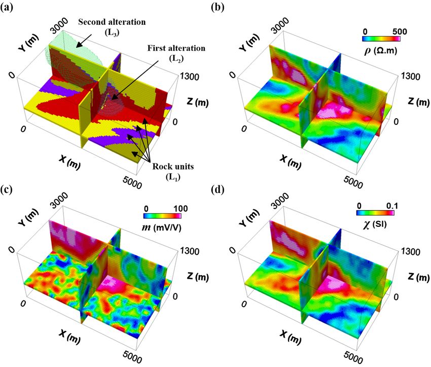
The basic lithology model was constructed from an original layered Earth model
passed through several faulting, folding, dyke intrusion, shear deformation, and alteration
overprints (Figures 2 and 3). The final 3D lithology model (stage 12 in Figure 3) included a
set of background rock units (L1a , L1b , L1c , L1d ) and two stages of hydrothermal alteration
in the form of plug-shaped alteration overprints (L2 and L3 ). Figure 4 represents the last
episode of the geological history stored as six independent lithotypes to be used later in
this study.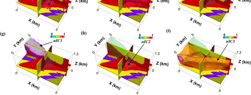
the last episode of the geological history stored as six independent lithotypes to be used
                                             later in this study.
                                                   The linear overlap of the four rock units and the two alteration events comprised
                                             three physical property distributions: electrical resistivity, induced polarization chargea-
          Minerals 2021, 11, 959             bility, and magnetic susceptibility. A mixing system was built to simulate a disseminated
                                                                                                                                    8 of 20
                                             sulfide deposit, where background rock units are intruded by two distinct disseminated
                                             sulfide-rich alteration events with the following mixing matrix form (Equation (1)).

            Figure
            Figure 2.2. Workflow of geological
                        Workflow of geological model
                                                 model construction.
                                                        construction. The
                                                                      The background
                                                                          background geology
                                                                                     geology consisted
                                                                                              consisted of
                                                                                                        of aa three-layer
                                                                                                               three-layerstratum
                                                                                                                           stratum(L  (L1a1a,, LL1b
                                                                                                                                                 1b,,

            L  )
x FOR PEER REVIEW
             1c  intruded  by a dyke (L1d ). After several faulting and shear deformation, two alteration  events  (L 2 and L 3 ) and  further
            L1c ) intruded by a dyke (L1d ). After several faulting and shear deformation, two alteration events (L2 and L3 ) and further 9 of 21
            deformations overprinted the host geology. Noddy 3D geological and geophysical modeling package was used to build
            deformations overprinted the host geology. Noddy 3D geological and geophysical modeling package was used to build the
            the geological model [43].
            geological model [43].

                Figure 3. Construction
                     Figure             of geological
                             3. Construction          features. Reference
                                                 of geological   features.  geological
                                                                               Reference  model  was selected
                                                                                              geological       at thewas
                                                                                                           model      endselected
                                                                                                                          of stage 12
                                                                                                                                    atwith
                                                                                                                                       the three
                                                                                                                                           end of
                major geological features: a background geology (L1a , L1b , L1c , L1d ) and two separate alteration overprints overlapped over
                     stage 12 with three major geological features: a background geology (L1a, L1b, L1c, L1d) and two sepa-
                the background geological features (L2 , L3 ).
                      rate alteration overprints overlapped over the background geological features (L2, L3).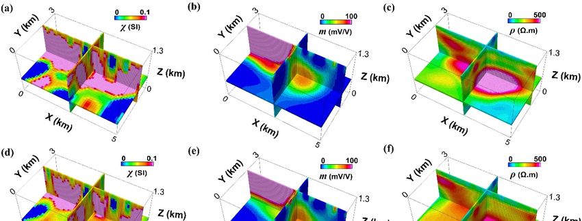
Minerals 2021, 11, 959 Figure 3. Construction of geological features. Reference geological model was selected at the end
9 of of
20
stage 12 with three major geological features: a background geology (L1a, L1b, L1c, L1d) and two sepa-
rate alteration overprints overlapped over the background geological features (L2, L3).
Figure 4. Three independent geological features contribute to the bulk physical properties (a). The background lithology
has three components (b–d), which is intruded by a dyke (e) and overprinted by two successive alteration events (f).
The linear overlap of the four rock units and the two alteration events comprised three
physical property distributions: electrical resistivity, induced polarization chargeability,
and magnetic susceptibility. A mixing system was built to simulate a disseminated sulfide
deposit, where background rock units are intruded by two distinct disseminated sulfide-
rich alteration events with the following mixing matrix form (Equation (1)).
L1 L2 L3
↓ ↓ ↓
0.9 0.05 0.05 → ρ = 0.90L1 + 0.05L2 + 0.05L3 (14)
A = 0.5 0.2 0.75 → m = 0.05L1 + 0.20L2 + 0.75L3
0.45 0.25 0.3 → χ = 0.45L1 + 0.25L2 + 0.30L3
Equation (14) means that 90 percent of the first physical property (P1 = ρ; electric
resistivity) is derived from the background rocks (L1a , L1b , L1c , L1d ), 5 percent from the
alteration L2 , and 5 percent from the alteration L3 . The second physical property is induced
polarization chargeability (P2 = m), which is least sensitive to the background geology
(5 percent), and 20 percent and 75 percent of it result from the two alteration events
(L2 and L3 ). Note that 75 percent of chargeability comes from the alteration L3 , which
means L3 bears the largest amount of disseminated sulfides. The magnetic susceptibility
(P3 = χ) represents 45 percent of the background geology, 25 percent the alteration L2
and 30 percent the alteration L3 . The resulting mixtures were then scaled from zero
to a reasonable maximum; set to 500 Ohm-m, 100 mV/V, and 0.1 SI for resistivities,
chargeabilities, and susceptibilities.
Figure 5 shows the calculated physical property models. An additional non-Gaussian
noise accompanies the mixing process to simulate a realistic geological environment where
the lithologies are heterogeneous. We used a Pearson random system to create this geologi-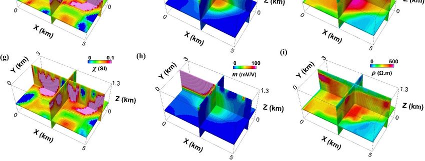
Minerals 2021, 11, 959                                                                                                              10 of 20

                                          cal noise in the form of a 3D matrix with unit standard deviation and skewness equal to
, x FOR PEER REVIEW                       1 for resistivity and chargeability models and skewness equal to −1 for the    susceptibility
                                                                                                                      11 of 21
                                          model. The kurtosis of the geological noise was set to 5 for the resistivity model and 4 for
                                          the chargeability and susceptibility models.

             FigureFigure    5. The system
                     5. The mixing    mixingproduces
                                               system three
                                                       produces    threephysical
                                                             overlapped    overlapped     physical
                                                                                    properties       properties
                                                                                               (ρ, m and χ in b–d)(ρ, m and
                                                                                                                   from       χ in geological
                                                                                                                         simulated b–d)
                   from
             features  (a).simulated    geological
                             Each physical          features
                                             property         (a). Each
                                                      distribution  shows physical
                                                                            a portionproperty   distribution
                                                                                       of the whole            shows
                                                                                                      geological       a portion
                                                                                                                 features         of the
                                                                                                                           (b–d). The  source
                   whole geological features (b–d). The source separation aims to recover the hidden independent fea-
             separation  aims   to recover the hidden independent    features to reconstruct the  whole geological  model.
                   tures to reconstruct the whole geological model.
                                             The histograms of the original litho-codes and the simulated physical properties are
                                        shown in Figure 6. As can be seen, the histograms of physical properties (Figure 6d–f) show
                         The histograms of the original litho-codes and the simulated physical properties are
                                        the multimodal nature of the physical properties due to the mixing process. However,
                   shown in Figure 6.   theAs   can non-Gaussian
                                            added    be seen, the histograms         of physical
                                                                      geological noise             properties
                                                                                         smooths some    smaller(Figure
                                                                                                                  patterns6d–f)
                                                                                                                            related to the
                   show the multimodal       nature
                                        overlaps       ofrock’s
                                                  of the  the physical
                                                                 units withproperties   dueepisodes
                                                                             two alteration  to the mixing    process.
                                                                                                      (Figure 6g–i).      How-
                                                                                                                     We also   predict that
                   ever, the added non-Gaussian          geological    noise  smooths     some  smaller   patterns   related
                                        the passage of lithological information from the geophysical system and then the       to imaging
                   the overlaps of thesystem
                                         rock’swill
                                                  units  with tworeduce
                                                     significantly    alteration  episodes (Figure
                                                                            this multimodality        6g–i). We
                                                                                                to bimodality     also unimodality.
                                                                                                              or even   predict       This
                                        information   loss is one  of the major  limitations of 3D  geophysical
                   that the passage of lithological information from the geophysical system and then the im-     imaging   that we  aim  to
                                        tackle in this study  quantitatively.
                   aging system will significantly reduce this multimodality to bimodality or even unimodal-
                                             This study used a three-component geological model and a three-component physical
                   ity. This information loss is one of the major limitations of 3D geophysical imaging that
                                        property model to avoid too many drawn-out interpretations. However, in practice, we can
                   we aim to tackle inuse this
                                            anystudy
                                                 number quantitatively.
                                                           of geological features and physical properties, including seismic velocities
                         This study usedand bulk densities, for 3Dgeological
                                            a  three-component                      model and
                                                                        seismic tomography    anda three-component       physi-
                                                                                                   gravity modeling. Nevertheless,       to
                   cal property model      to avoid
                                        avoid          too many
                                               inconsistency,    we drawn-out
                                                                    kept the numberinterpretations.
                                                                                        of geological However,     in practice,
                                                                                                      features equal   to or less than the
                   we can use any numberphysicalofproperties
                                                    geological (n ≤ m).
                                                                  features   and physical properties, including seismic
                   velocities and bulk densities, for 3D seismic tomography and gravity modeling. Never-
                   theless, to avoid inconsistency, we kept the number of geological features equal to or less
                   than the physical properties (n ≤ m).
x FOR PEER REVIEW
Minerals 2021, 11, 959 12 of 21 11 of 20
Figure 6. Histograms of simulated physical properties: (a–c) Histograms of the original litho-codes used for geological
Figure(d–f)
modeling; 6. Histograms
Histograms ofofthe
simulated physical
mixed physical properties:
properties (a–c)(g–i)
(noise-free); Histograms
Histograms ofofthe
theoriginal litho-codes
mixed physical properties
withused
addedfor geological modeling;
non-Gaussian (d–f) Histograms
noise. Multimodal of the mixed
nature of the physical physical
properties properties
is a result (noise-free);
of the mixing process. (g–i)
The solid
Histograms
curve indicates theofcumulative
the mixeddistribution
physical properties
function. with added non-Gaussian noise. Multimodal nature of
the physical properties is a result of the mixing process. The solid curve indicates the cumulative
distribution function.3.2. Petrophysical Feature Extraction
We evaluated different source separation algorithms to see which method was more
3.2. Petrophysical Feature Extraction
stable in the recovery of lithological factors in the presence of the non-Gaussian noise on
We evaluated the mixed physical
different source properties.
separationThe objective isto
algorithms tosee
recover
whichthe method
two separate
wasalteration
more events
from the background lithology, supposing that the imaging system has zero influence on
stable in the recovery of lithological factors in the presence of the non-Gaussian noise on
the source separation, equivalent to a situation where geophysical inversion accurately
the mixed physicalrecovers
properties. The
physical objective
properties. Thisisstrategy
to recover the us
will help two separate
to compare thealteration
exact results to the
events from the background lithology,
more realistic supposing
scenario of that the
an approximate imaging
inverse system
solution has zero the
to understand influ-
effect of the
ence on the sourcegeophysical
separation,andequivalent to a situation
imaging systems where
on the source geophysical
separation inversion ac-
process.
curately recovers physical properties. This strategy will help us to compare the exact re-
sults to the more realistic scenario of an approximate inverse solution to understand the
effect of the geophysical and imaging systems on the source separation process.
Running PCA to separate images did not yield efficient separate geological features,
and another form of mixture remained on the principal components (Figure 7a–c). EvenMinerals 2021, 11, x FOR PEER REVIEW 13 of 21
Minerals 2021, 11, 959 12 of 20
the first and third principal components (PC1 and PC3 in Figure 7a,c) successfully repre-
sent the background geology (L1) and the first alteration event (L2), but the third alteration
event (L3) is still mixed with the second alteration event in the second principal component
(PC2Running PCA
in Figure 7b).to separate images did not yield efficient separate geological features,
and another form
Fast-ICA by of mixture
kurtosis remained on
maximization the neither
could principal components
tolerate (Figure
the mixing 7a–c).
system’s Even if
added
the recovered
geological principal
noise, components
resulting of the physical
in few overlapped properties
features are uncorrelated,
in the separated knowing
outputs (Figure
the values
7d–f). of one Fast-ICA
However, image still
by provides
negentropyinformation
maximizationabout the other
recovered image. However,
the underlying geolog- the
first
icaland thirdalmost
features principal components
perfectly. (PC1
As can be seenand PC37g–i),
(Figure in Figure 7a,c) successfully
negentropy maximizationrepresent
can
efficiently handle the added non-Gaussian background geological noise separating
the background geology (L1 ) and the first alteration event (L2 ), but the third alteration the
main geological features.
event (L3 ) is still mixed with the second alteration event in the second principal component
(PC2 in Figure 7b).
Figure
Figure 7. Assessment
7. Assessment ofofdifferent
differentsource
source separation
separationmethods:
methods: (a–c) principal
(a–c) components
principal components (PC1,(PC1,
PC2, and PC3)
PC2, andfrom
PC3)thefrom
PCA method;
the PCA method; (d–f)
(d–f)independent
independent components
components (kIC1, kIC2,kIC2,
(kIC1, and kIC3) from Fast-ICA
and kIC3) by kurtosis
from Fast-ICA maximization;
by kurtosis (g–i) inde-(g–i)
maximization;
pendent components (nIC1, nIC2 and nIC3) from Fast-ICA by negentropy maximization. PCA recreates another set of
independent components (nIC1, nIC2 and nIC3) from Fast-ICA by negentropy maximization. PCA recreates another set of
overlapped images on PC2 and is ineffective in source separation (a–c). Fast-ICA by kurtosis maximization produces a set
overlapped
of imagesimages
(kICs) on PC2 and
separated to is ineffective
some in source
extent, but separation
still, some (a–c). remain
of the features Fast-ICA by kurtosis
mixed maximization
in the first produces a set
and second independent
of images (kICs) in
components separated
the form to some extent,
of outliers, but still,
background some of
geology the features
mixed with the remain mixed in event.
second alteration the first and second
Fast-ICA independent
by negentropy
maximization
components in theproduces a set of images
form of outliers, (nICs) that
background are efficiently
geology mixed with separated (g–i).alteration
the second All principal and Fast-ICA
event. independent compo-
by negentropy
nents wereproduces
maximization normalized from
a set zero to one
of images forthat
(nICs) consistency of visualization.
are efficiently separated (g–i). All principal and independent components
were normalized from zero to one for consistency of visualization.
Fast-ICA by kurtosis maximization could neither tolerate the mixing system’s added
geological noise, resulting in few overlapped features in the separated outputs (Figure 7d–f).
However, Fast-ICA by negentropy maximization recovered the underlying geological
features almost perfectly. As can be seen (Figure 7g–i), negentropy maximization can
efficiently handle the added non-Gaussian background geological noise separating the
main geological features.Minerals
Minerals 2021,
2021, 11, 11,
959x FOR PEER REVIEW 14 of1321
of 20
3.3. Simulation of the Geophysical System (Forward Modeling)
3.3. Simulation of the Geophysical System (Forward Modeling)
We calculated the geophysical responses of the mixed physical properties to explore
We calculated the geophysical responses of the mixed physical properties to explore
how the interdependent physical properties appear as geophysical signals on the surface
how the interdependent physical properties appear as geophysical signals on the surface of
of the Earth. This is a more realistic assumption because most geophysical data are gath-
the Earth. This is a more realistic assumption because most geophysical data are gathered on
ered on the surface and are apparent indicators of 3D underground physical property
the surface and are apparent indicators of 3D underground physical property distributions.
distributions.
The
TheDC/IP
DC/IP apparent physicalproperties
apparent physical propertieswereweresimulated
simulated over
over thethe mixed
mixed physical
physical
properties with pole–dipole electrode configurations, dipolar spacing
properties with pole–dipole electrode configurations, dipolar spacing of 100 m, and dipo- of 100 m, and dipolar
separations
lar separations up to
up12 times
to 12 timesin in
XX and
andYYdirections.
directions. The modelmesh
The model meshconsists
consists of of
151151 cells
cells
ininthethe X direction, 111 cells in the Y direction, and 38 cells in the Z direction with twotwo
X direction, 111 cells in the Y direction, and 38 cells in the Z direction with
nodes
nodesbetween
betweenthe theadjacent
adjacentelectrodes,
electrodes,which
which simulates
simulates thethe forward
forward electrical potentials of
electrical potentials
51ofelectrodes
51 electrodes in the X direction and 31 electrodes in the Y direction. Therefore, thethe
in the X direction and 31 electrodes in the Y direction. Therefore, total
total
number of electrodes is 1581, over a 3D discretized volume with 636918
number of electrodes is 1581, over a 3D discretized volume with 636918 rectangular cells. rectangular cells.
The
Thesame
same magnetic
magnetic station intervalswere
station intervals wereapplied
appliedfor formagnetic
magnetic forward
forward modeling,
modeling,
i.e.,
i.e., 100 m spacing between observation points in both the X and Y directions. Themagnetic
100 m spacing between observation points in both the X and Y directions. The mag-
field ◦ and
neticover
fieldthe 3Dthe
over volume
3D volume is setistoset
29,639 nT with
to 29,639 inclination
nT with andand
inclination declination
declination ofof
2121°
◦
1 and
, respectively. We assumed that that
there is no
1°, respectively. We assumed there is remanent
no remanent magnetization
magnetization contributing
contributingto tothe
surface observations
the surface observationsandand thatthat
demagnetization
demagnetization of rocks
of rocksis negligible.
is negligible.
We
Wecalculated
calculated thethe forward responses over
forward responses overthethe3D 3Drectangularly
rectangularlygridded
gridded physical
physical
properties
propertiesusingusing forward
forward modeling algorithmsintroduced
modeling algorithms introduced inin
LiLi
andand Oldenburg
Oldenburg [29,30].
[29,30].
Figure88shows
Figure showsthetheforward
forward responses
responses of of the
the magnetic
magneticand andDC/IP
DC/IP models
models in in
thethe
form
formof of
totalmagnetic
total magneticfield
fieldintensities
intensities(after
(afterreduction
reductiontotomagnetic
magneticpole),
pole),apparent
apparentresistivities,
resistivities,and
and apparent
apparent chargeabilities.
chargeabilities.
Figure
Figure 8. The
8. The geophysicalresponses
geophysical responses(S(Sd )d)of
ofthe
the mixed
mixed physical
physical properties
properties(P
(Pj):j ):(a)
(a)total
totalmagnetic
magneticfield intensities
field after
intensities after
reduction to magnetic pole; (b) apparent resistivities; (c) apparent chargeabilities. DC/IP responses are
reduction to magnetic pole; (b) apparent resistivities; (c) apparent chargeabilities. DC/IP responses are presented on presented on twotwo
NS and EW pseudo-sections as well as a horizontal slice corresponding to the dipolar separation of n = 9. The arrows
NS and EW pseudo-sections as well as a horizontal slice corresponding to the dipolar separation of n = 9. The arrows (black)
(black) indicate the location of simulated DC/IP electrodes.
indicate the location of simulated DC/IP electrodes.
3.4. Imaging System (Inverse Modeling)
3.4. Imaging System (Inverse Modeling)
One of the main objectives of this study was exploring the sensitivity of feature ex-
Onetoofthe
traction the mainofobjectives
tuning the imaging ofsystem.
this study was inverse
Through exploring the sensitivity
modeling of feature
(imaging system),
extraction
we soughttotothe tuning
recover the of the imaging
physical propertiessystem. Through
with different inverse modeling
adjustments (imaging
of the inversion
system), we sought
parameters. Finally, to
werecover
unmixed the physical
the recovered properties
physical with different
properties adjustments
(in the unmixing sys-of the
inversion parameters.theFinally,
tem) to approximate we unmixed
underlying lithologicalthe recovered
factors. physicalhow
We evaluated properties (in the
the imaging
unmixing system) to
system (inversion) approximate
can the underlying
distort the unmixing processlithological factors. We
during the inference evaluated
of the lithologi-how
the
calimaging system the
factors. Though (inversion) can distort
mixing system thelinearly,
behaves unmixing theprocess duringresponse
Earth forward the inference
(geo- of
physical
the systemfactors.
lithological in Figure 1), and the
Though the mixing
reconstruction
systemofbehaves
physicallinearly,
propertiesthe(imaging sys-
Earth forward
tem in Figure 1) add unwanted artifacts to the inverted physical property
response (geophysical system in Figure 1), and the reconstruction of physical properties images, specif-
ically when
(imaging we executed
system in Figureunconstrained
1) add unwanted3D inversions
artifactsdue
to to
thethe lack of prior
inverted petrophys-
physical property
ical information.
images, specifically when we executed unconstrained 3D inversions due to the lack of prior
petrophysical information.
A set of underlying inversion parameters were set to recover sharp images of the
physical properties. The blocky DC/IP inversion was controlled by different cut-off factorsMinerals 2021, 11, x FOR PEER REVIEW 15 of 21
A set of underlying inversion parameters were set to recover sharp images of the
Minerals 2021, 11, 959 physical properties. The blocky DC/IP inversion was controlled by different cut-off14factors of 20
to examine the effect of inversion artifacts on the outputs of the feature extraction algo-
rithm. Achieving a value too close to the l2-norm criteria (larger cut-off factors) increased
thetomisfit
examine error,
the and
effectcloser to l1-norm
of inversion (smaller
artifacts on thecut-off
outputs factors) produced
of the feature too sharp
extraction bound-
algorithm.
aries
Achieving a value too close to the l -norm criteria (larger cut-off factors) increasedDC/IP
that distorted the 3D continuity 2 of the models. We used three representative the
inversion episodes
misfit error, withtothe
and closer following
l1 -norm parameters:
(smaller the first
cut-off factors) DC/IP too
produced inversion with a data
sharp boundaries
constraint cut-offthefactor
that distorted k1 = 1 andofathe
3D continuity model constraint
models. We used cut-off
threefactor k2 = 1 (smoothest
representative DC/IP
physical properties); the second DC/IP inversion with k1 = 0.1 and k2 = 0.05 (sharper
inversion episodes with the following parameters: the first DC/IP inversion with a data
constraint
physical cut-off factor
properties); k1 = 1DC/IP
the third and a model
inversionconstraint
with k1cut-off and kk22 == 0.005
= 0.01factor 1 (smoothest
(sharpest
physical
physical properties); the second DC/IP inversion with k1 = 0.1 and k2 = 0.05 (sharper
properties).
physical
Three properties); the third DC/IP
episodes (iterations) with k1 = 0.01
inversionreweighing
of the iterative and k2inversion
magnetic = 0.005 (sharpest
were also
physical properties).
used to produce three smooth-to-sharp representative susceptibility models. The recov-
Three episodes
ered physical properties(iterations)
(Figure 9) ofexhibit
the iterative reweighing
valuable informationmagnetic
about inversion were also
the underlying fea-
used to produce three smooth-to-sharp representative susceptibility models. The recovered
tures, but some of the key background geological features are missed due to the imaging
physical properties (Figure 9) exhibit valuable information about the underlying features,
process. The first imaging scenario (smoothest) was tuned to recover approximations of
but some of the key background geological features are missed due to the imaging process.
physical
The firstproperties (ρ, m, and
imaging scenario χ), wherewas
(smoothest) thetuned
sharpness of images
to recover was enough
approximations to capture
of physical
anproperties
overall view ofand
(ρ, m, the χ),
underlying
where thegeological
sharpness features
of images(Figure
was enough9a–c).toHowever,
capture anincreasing
overall
theview
depth of investigation in the smooth inversions deforms
of the underlying geological features (Figure 9a–c). However, increasing the shape of the the
firstdepth
altera-
tion event that is in
of investigation thethedeepest
smoothone (L2 in Figure
inversions deforms4f).the
Increasing
shape of the the first
levelalteration
of sharpness
event in
Figure
that is9d–f
the focuses
deepest moreone (Lon 2 inthe hidden
Figure 4f). geological
Increasing features.
the level However,
of sharpness theintwo alteration
Figure 9d–f
events
focusesaremore
still attached. The sharpest
on the hidden geological images are presented
features. However, the in Figure 9g–i, where
two alteration eventstheare
lith-
ological background is much more visible in the resistivity and susceptibility images (Fig-
still attached. The sharpest images are presented in Figure 9g–i, where the lithological
urebackground
9g–i), and two is much more visible
alteration eventsinarethemore
resistivity and in
confined susceptibility
the modeled images (Figure 9g–i),
chargeability image
and two
(Figure alteration events are more confined in the modeled chargeability image (Figure 9h).
9h).
Figure 9. Geophysical
Figure inversion
9. Geophysical results:
inversion (a–c)
results: smooth
(a–c) inversion
smooth results;
inversion (d–f)
results; sharper
(d–f) inversion
sharper inversionresults;
results;(g–i)
(g–i)sharpest
sharpestin-
version results.
inversion results.Minerals 2021, 11, 959 15 of 20
Minerals 2021, 11, x FOR PEER REVIEW 16 of 21
3.5.
3.5.Post-Inversion
Post-Inversion Feature Extraction
Feature Extraction
We
Weevaluated
evaluatedthetheeffect
effectofofimaging
imagingsystems
systems (inverse
(inverse modeling)
modeling) on on the
the performance
performance of
feature
of feature extraction. We explored different inversion procedures to investigatehow
extraction. We explored different inversion procedures to investigate howartifacts
arti-
from
facts from the imaging system leak into the estimated physical properties and thendistort
the imaging system leak into the estimated physical properties and then distortthe
performance
the performanceof geological
of geological feature extraction.
feature WeWe
extraction. do donotnot
showshow thetheresults ofof
results thethePCA
PCAand
ICA by kurtosis maximization because we already showed that
and ICA by kurtosis maximization because we already showed that they were not as effi-they were not as efficient
ascient
the as
negentropy maximization
the negentropy maximization algorithm. TheThe
algorithm. major
major difference
difference between
betweenpre-inversion
pre-inver-
(petrophysical) and post-inversion
sion (petrophysical) and post-inversion feature extraction
feature is thatisthe
extraction thatdepth estimation
the depth in the in
estimation post-
inversion physical properties
the post-inversion leads to distorted
physical properties physical physical
leads to distorted propertyproperty
images and imageserroneous
and
reconstructed geological features.
erroneous reconstructed geological features.
The
Thepost-inversion featureextraction
post-inversion feature extraction results
results areare
shownshown in Figure
in Figure 10 for10the
for the in-
three three
inversion scenarios.The
version scenarios. Theindependent
independent components
components of ofthethe smoothest
smoothest physical
physical properties
properties
(Figure
(Figure10a–c)
10a–c)keep
keep some
some of the latent
latentfeatures
featuresmixed,
mixed,whichwhichis is understandable
understandable due due to the
to the
smoothness artifacts
smoothness artifacts leaked
leaked into
into the
the imaging
imagingand andfeature
featureextraction
extraction systems.
systems.TheThe third
third
alteration event is clearly extracted in the second independent component
alteration event is clearly extracted in the second independent component (nIC2), but the (nIC2), but the
background geology
background geology and the the first
first alteration
alterationevent
eventwere
weremixed
mixedinin the
theother
otherindependent
independent
components (nIC1
components (nIC1 and and nIC3).
Figure 10. Post-inversion Figure
feature10.extraction
Post-inversion feature
through extraction through
negentropy negentropy
maximization maximization
on different on different
inversion inver-
scenarios:
sion scenarios: (a–c) independent components of smoothest physical properties;
(a–c) independent components of smoothest physical properties; (d–f) independent components of sharper physical(d–f) independent
components of sharper physical properties; (g–i) independent components of sharpest physical
properties; (g–i) independent components of sharpest physical properties.
properties.
Running a sharper inversion helped to increase the contrast of the models. How-
ever, a certain amount of information is still lost during the imaging process. Again, theYou can also read