A seamless ensemble-based reconstruction of surface ocean pCO2 and air-sea CO2 fluxes over the global coastal and open oceans
←
→
Page content transcription
If your browser does not render page correctly, please read the page content below
Research article
Biogeosciences, 19, 1087–1109, 2022
https://doi.org/10.5194/bg-19-1087-2022
© Author(s) 2022. This work is distributed under
the Creative Commons Attribution 4.0 License.

A seamless ensemble-based reconstruction of surface ocean pCO2
and air–sea CO2 fluxes over the global coastal and open oceans
Thi Tuyet Trang Chau, Marion Gehlen, and Frédéric Chevallier
Laboratoire des Sciences du Climat et de l’Environnement, LSCE-IPSL, CEA-CNRS-UVSQ, Université Paris-Saclay,
91191 Gif-sur-Yvette, France

Correspondence: Thi Tuyet Trang Chau (trang.chau@lsce.ipsl.fr)

Received: 30 July 2021 – Discussion started: 3 August 2021
Revised: 21 December 2021 – Accepted: 21 January 2022 – Published: 21 February 2022

Abstract. We have estimated global air–sea CO2 fluxes            of 0.526 ± 0.022 PgC yr−1 over the 35-year period. The link
(fgCO2 ) from the open ocean to coastal seas. Fluxes and as-     between the large interannual to multi-year variations of the
sociated uncertainty are computed from an ensemble-based         global net sink and the El Niño–Southern Oscillation climate
reconstruction of CO2 sea surface partial pressure (pCO2 )       variability is reconfirmed.
maps trained with gridded data from the Surface Ocean CO2
Atlas v2020 database. The ensemble mean (which is the
best estimate provided by the approach) fits independent data
well, and a broad agreement between the spatial distribu-        1   Introduction
tion of model–data differences and the ensemble standard
deviation (which is our model uncertainty estimate) is seen.     Since the onset of the industrial era, humankind has pro-
Ensemble-based uncertainty estimates are denoted by ±1σ .        foundly modified the global carbon (C) cycle. The use of
The space–time-varying uncertainty fields identify oceanic       fossil fuels, cement production, and land use change added
regions where improvements in data reconstruction and ex-        700±75 PgC (best estimate ±1σ ) to the atmosphere between
tensions of the observational network are needed. Poor re-       1750 and 2019 (Friedlingstein et al., 2020). An estimated
constructions of pCO2 are primarily found over the coasts        285 ± 5 PgC of this excess C stayed there; the remainder was
and/or in regions with sparse observations, while fgCO2 esti-    taken up by the ocean (170 ± 20 PgC) and the land biosphere
mates with the largest uncertainty are observed over the open    (230 ± 60 PgC). While the fraction of total CO2 emissions
Southern Ocean (44◦ S southward), the subpolar regions, the      sequestered by the ocean has remained rather stable (22 %–
Indian Ocean gyre, and upwelling systems.                        25 %) over the past 6 decades (Friedlingstein et al., 2020),
   Our estimate of the global net sink for the period            the global ocean sink has varied significantly at interannual
1985–2019 is 1.643 ± 0.125 PgC yr−1 including 0.150 ±            timescales (Rödenbeck et al., 2015). Global ocean biogeo-
0.010 PgC yr−1 for the coastal net sink. Among the ocean         chemical models (GOBMs) are used within the framework of
basins, the Subtropical Pacific (18–49◦ N) and the Subpolar      the annual assessment of the global carbon budget (Friedling-
Atlantic (49–76◦ N) appear to be the strongest CO2 sinks for     stein et al., 2020) to annually re-estimate the means of and
the open ocean and the coastal ocean, respectively. Based on     variations in CO2 sinks and sources over the global ocean
mean flux density per unit area, the most intense CO2 draw-      and major basins. However, these recent model-based esti-
down is, however, observed over the Arctic (76◦ N poleward)      mates need to be benchmarked against observation-based es-
followed by the Subpolar Atlantic and Subtropical Pacific for    timates in order to better understand the global carbon budget
both open-ocean and coastal sectors. Reconstruction results      as well as its yearly re-distribution in the biosphere (Hauck
also show significant changes in the global annual integral of   et al., 2020).
all open- and coastal-ocean CO2 fluxes with a growth rate of        In situ measurements of sea surface fugacity of CO2 col-
+0.062 ± 0.006 PgC yr−2 and a temporal standard deviation        lected by an international coordinated effort of the ocean ob-
                                                                 servation community and combined into the Surface Ocean

Published by Copernicus Publications on behalf of the European Geosciences Union.
1088                                                               T. T. T. Chau et al.: pCO2 and air–sea CO2 flux estimates

CO2 Atlas (SOCAT, https://www.socat.info/, last access:            quantification of an averaged pCO2 or an integrated flux over
16 June 2020; Bakker et al., 2016) provide an observational        the space and time of interest is with low confidence due to
constraint on the assessment of the surface ocean partial pres-    sparse data density. Also, most of the aforementioned map-
sure of CO2 (pCO2 ) and the ocean C sinks and sources. De-         ping methods target pCO2 data and estimate air–sea fluxes
spite an increasing number of observations since the 1990s,        solely over the open ocean, with the coastal data excluded
data density remains uneven in space and time. While, for          or not fully qualified. In Laruelle et al. (2014), the authors
instance, data coverage is sparse over the southern basins of      present spatial distributions of air–sea flux density and esti-
the Atlantic and Pacific oceans, observations are seasonally       mates of the total coastal C sink inferred from spatial integra-
biased towards the summers at high latitudes (Landschützer         tion methods on coastal SOCAT data. Laruelle et al. (2017)
et al., 2014; Denvil-Sommer et al., 2019; Gregor et al., 2019).    adapted the two-step neural network approach described in
   Various data-based approaches have been proposed to in-         Landschützer et al. (2016) to the coastal-ocean pCO2 . The
fer gridded maps of surface ocean pCO2 from the sparse             coastal and open-ocean products were combined into a sin-
set of observation-based data. They have been successful           gle reconstruction to yield a global monthly climatology of
in obtaining similarly low misfits between the reconstructed       pCO2 presented in Landschützer et al. (2020). Notwithstand-
and evaluation data and reasonable estimates of air–sea CO2        ing these advances, a global reconstruction and its uncer-
fluxes (see Rödenbeck et al., 2015; Gregor et al., 2019;           tainty assessment of monthly varying coastal surface ocean
Friedlingstein et al., 2020) although model design and im-         pCO2 and air–sea fluxes are still missing.
plementation are quite different (e.g. the proportion of SO-          In this work, we propose a new inference strategy for re-
CAT data used in model fitting and evaluation). Aside from         constructing the monthly pCO2 fields and the contempo-
data reconstruction built on a single model mapping pCO2           rary air–sea fluxes over the period 1985–2019 with a spa-
data with machine learning, classical regression, or mixed-        tial resolution of 1◦ × 1◦ . It is based on a Monte Carlo ap-
layer schemes (e.g. Rödenbeck et al., 2013; Landschützer           proach, an ensemble of 100 neural network models mapping
et al., 2016; Iida et al., 2021), ensemble-based approaches        sub-samples drawn from the monthly gridded SOCATv2020
have recently emerged but with their own concepts and ob-          data and available data of predictors. This ensemble ap-
jectives. For example, Denvil-Sommer et al. (2019) designed        proach was developed at the Laboratoire des Sciences du
a two-step reconstruction of pCO2 climatologies and anoma-         Climat et de l’Environnement (LSCE) as both an extension
lies based on five neural network models and selected the one      of and an improvement on the first version (LSCE-FFNN-
that reproduced the pCO2 field with the smallest model–data        v1; Denvil-Sommer et al., 2019). In the following sections,
misfit. Gregor et al. (2019) and Gregor and Gruber (2021)          we first present the ensemble of neural networks designed
introduced machine-learning ensembles with 6 to 16 differ-         with the aims of leaving aside the issue of discrete bound-
ent two-step clustering–regression models mapping surface          aries in the existing two-step clustering–regressions (see fur-
pCO2 and suggest that the use of their ensemble mean is            ther discussion in Gregor and Gruber, 2021) and reducing
better than each member estimate. In a broader context, Rö-        the mapping uncertainties induced by the two-step recon-
denbeck et al. (2015) presented an intercomparison of 14           struction of the pCO2 fields (Denvil-Sommer et al., 2019) or
mapping methods targeting the identification of common or          by an ensemble-based reconstruction with a small ensemble
distinguishable features of different products in long-term        size. In addition, each feed-forward neural network (FFNN)
mean, regional, and temporal variations. Hauck et al. (2020)       model follows a leave-p-out cross-validation approach, i.e.
and Friedlingstein et al. (2020) also synthesized pCO2 map-        the exclusion of p gridded SOCAT data of the reconstructed
ping products and took an ensemble of their observation-           month itself in model training and validation. This allows us
based estimates of air–sea CO2 fluxes as a benchmark to            to reduce model over-fitting and to leave many more inde-
compare with the one derived from ocean biogeochemical             pendent data for model evaluation than in the previous stud-
models.                                                            ies. The mean and standard deviation computed from the en-
   Despite positive conclusions overall, statistical data recon-   semble of 100 model outputs are defined as estimates of the
structions are still subject to further improvements. In Rö-       mean state and uncertainty in the carbon fields. As one of
denbeck et al. (2015), Hauck et al. (2020), Bushinsky et al.       the novel key findings of this study compared to the exist-
(2019), and Denvil-Sommer et al. (2021), the authors explain       ing ones, we compute and analyse the estimates of pCO2
that substantial extensions of surface ocean observational         and air–sea fluxes, model errors, and model uncertainties for
network systems are essential to better determine pCO2 and         different timescales (e.g. monthly, yearly, and multi-decadal)
fluxes at finer scales and reduce mapping uncertainties. So far    and spatial scales (e.g. grid cells, sub-basins, and the global
mapping uncertainties have been estimated by using misfits         ocean). We then suggest the use of an indicator map built on
between the model outputs and SOCAT data (e.g. the root-           the space–time-varying uncertainty fields instead of model–
mean-square deviation, RMSD). By construction, such un-            data misfits for identifying regions that should be prioritized
certainty estimates are restricted to oceanic regions and peri-    in future observational programmes and model development
ods when observations are available (Rödenbeck et al., 2015;       in order to improve data reconstruction. Last but not least, the
Lebehot et al., 2019; Gregor et al., 2019), and the uncertainty    model best estimates of and uncertainty in pCO2 and air–

Biogeosciences, 19, 1087–1109, 2022                                                   https://doi.org/10.5194/bg-19-1087-2022
T. T. T. Chau et al.: pCO2 and air–sea CO2 flux estimates                                                                     1089

sea fluxes are analysed seamlessly over the open ocean to          instance, chl a was set approximately to 0 mg m−3 over the
the coastal zone. Potential drivers of the spatio-temporal dis-    Arctic and the Southern Ocean winter when no data were
tribution and the magnitude of open-ocean and coastal CO2          available. In the case of data being unavailable before 1998,
fluxes are discussed with the aim to better identify underly-      climatologies based on all available data were used as pre-
ing processes and to detect potential focus regions for further    dictors. Exceptionally, predictors for SSH before 1993 were
studies on the evolution of oceanic CO2 sources and sinks.         climatologies plus a linear trend in order to retain the overall
                                                                   response to the global warming. The MLD before 1992 was
                                                                   taken as the average MLD between 1992 and 1997.
2     Methods                                                         An ensemble of 100 FFNN models was used to recon-
                                                                   struct monthly pCO2 fields with a 1◦ × 1◦ resolution over
2.1    General formulation
                                                                   the global surface ocean during the years 1985–2019. This
The air–sea flux density (molC m−2 yr−1 ) is calculated here       ensemble approach was developed at the Laboratoire des Sci-
by the standard bulk equation                                      ences du Climat et de l’Environnement (LSCE) as both an
                                                                   extension of and an improvement on the first version (LSCE-
fgCO2 = kL (1 − fice ) 1pCO2                                       FFNN-v1; Denvil-Sommer et al., 2019). Our model outputs
        = kL (1 − fice ) pCOatm

                            2 − pCO2 ,                      (1)    are part of the Copernicus Marine Environment Monitoring
where k is the gas transfer velocity computed as a function        Service (CMEMS). Throughout the paper, it is hence referred
of the 10 m ERA5 wind speed (Hersbach et al., 2020) fol-           to as CMEMS-LSCE-FFNN.
lowing Wanninkhof (2014) and its coefficient is scaled to             To reconstruct the pCO2 fields over the global ocean for
match a global mean transfer velocity of 16.5 cm h−1 (Nae-         each target month over the 1985–2019 period, all the avail-
gler, 2009). L is the temperature-dependent solubility of CO2      able SOCAT data and the co-located predictors have been
(Weiss, 1974), fice and pCOatm                                     collected for the month before and the month after the tar-
                               2 are the sea-ice fraction and
the atmospheric CO2 partial pressure, respectively. In Eq. (1),    get month. We randomly extracted two-thirds of each one
a positive (negative) flux indicates oceanic CO2 uptake (re-       of these datasets to make training datasets for the FFNN
lease). Details and references for the source of these variables   models, leaving the remaining third to be corresponding test
are given in Table S1 in the Supplement, except for pCO2 ,         datasets. The FFNN models were then trained for each target
which is described in the following section.                       month. Moreover, the exclusion of the reconstructed month
                                                                   itself in the training and test datasets follows a leave-p-out
2.2    An ensemble-based approach for the                          cross-validation approach, where p is the number of gridded
       reconstruction of sea surface pCO2 and air–sea              SOCAT data in the target month. This approach allows us to
       CO2 fluxes                                                  reduce model over-fitting, as well as to assess the quality of
                                                                   the reconstruction against SOCAT data that are fully inde-
The sea surface partial pressure of CO2 in Eq. (1) is es-          pendent from the training phase.
timated monthly over each point of the global ocean by                The random extraction and the FFNN training were re-
analysing sparse in situ measurements of CO2 fugacity, gath-       peated 100 times so that 100 versions of the monthly FFNN
ered and gridded at a monthly and 1◦ resolution in the 2020        models have been obtained. Note that our ensemble approach
release of the Surface Ocean CO2 Atlas (SOCATv2020,                belongs to the classes of bootstrapping and Monte Carlo
https://www.socat.info/, last access: 16 June 2020). SO-           methods in statistics. Theoretically, the number of samples
CATv2020 covers the period 1985–2019. First, monthly               or the ensemble size must be substantially large to obtain
gridded pCO2 data were converted from SOCATv2020 CO2               a convergence. However, it was demonstrated in the litera-
fugacity (Körtzinger, 1999). We then regressed these pCO2          ture (e.g. Goodhue et al., 2012; Efron et al., 2015) that with
values against a set of predictors with non-linear functions,      an ensemble size of 50 the model estimation is likely sta-
i.e. feed-forward neural network (FFNN) models. As illus-          ble and with an ensemble size over 100 the improvement in
trated in Fig. 1, our predictors are biological, chemical, and     standard errors between model outputs and evaluation data
physical variables commonly associated with the variations         is negligible. Figure S2 in the Supplement shows an illus-
in pCO2 (e.g. Landschützer et al., 2013; Denvil-Sommer             tration of the reconstruction skill with respect to the ensem-
et al., 2019; Gregor et al., 2019): sea surface height (SSH),      ble size S. For each ensemble of S model outputs of pCO2
sea surface temperature (SST), sea surface salinity (SSS),         (S ∈ {5, 10, 20, 50, 75, 100}), the root-mean-square devia-
mixed-layer depth (MLD), chlorophyll a (chl a), and atmo-          tion (RMSD) is computed between the ensemble mean (our
spheric CO2 mole fraction (xCO2 ). A pCO2 climatology              best model estimate) and SOCAT data over the period 1985–
(Takahashi et al., 2009) and the geographical coordinates          2019. As seen in this figure, the reconstruction starts to stabi-
(latitude and longitude) were also added to the predictors. Ta-    lize with S = 50. In this study, we have exploited a large but
ble S1 details the data source. All data were reprocessed and      realistic amount of computing resources to run an ensemble
co-located at the same SOCAT resolution following Land-            of S = 100 neural network models. Equation (1) was then ap-
schützer et al. (2016) and Denvil-Sommer et al. (2019). For

https://doi.org/10.5194/bg-19-1087-2022                                                   Biogeosciences, 19, 1087–1109, 2022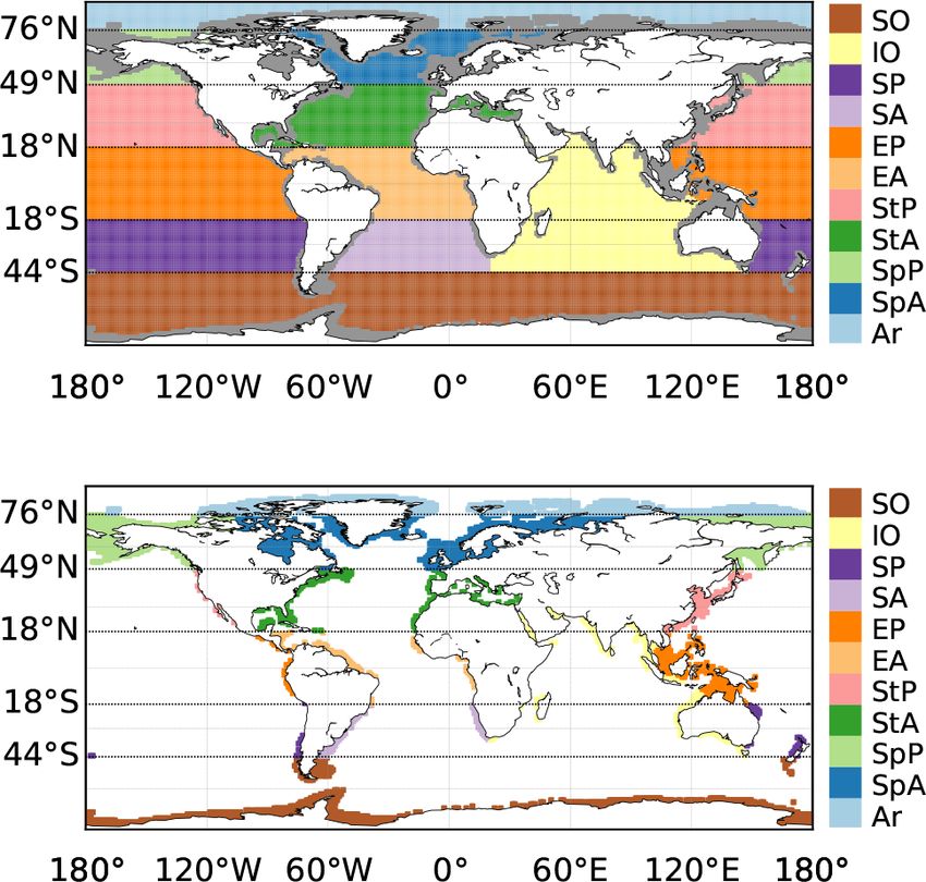
1090                                                               T. T. T. Chau et al.: pCO2 and air–sea CO2 flux estimates

Figure 1. Illustration of a feed-forward neural network (FFNN) model mapping monthly gridded SOCAT data and feature variables (Ta-
ble S1) co-located at a spatial resolution of 1◦ × 1◦ .

plied to the ensembles of FFNN outputs of pCO2 in order to         Table 1. Indication of 11 RECCAP1 regions (Fig. 2). Only the total
obtain ensembles of monthly global fgCO2 fields.                   area with respect to the maximum coverage of the reconstructed
                                                                   data is accounted for in each region.
2.3    Coastal and regional division
                                                                    Index   Region                        Latitude      Area (106 km2 )
The reconstructed pCO2 fields and air–sea CO2 fluxes are                                                                Open         Coast
analysed over the global ocean, at particular locations, and                                                            ocean
in 11 oceanic sub-basins used by the Regional Carbon Cy-                    Globe (G)                     90◦ S–90◦ N   330.42       22.35
cle Assessment and Processes Tier 1 (RECCAP1; Canadell              1       Arctic (Ar)                   76–90◦ N        1.07        0.99
et al., 2011) and previous studies (Schuster et al., 2013;          2       Subpolar Atlantic (SpA)       49–76◦ N        8.88        4.15
Sarma et al., 2013; Ishii et al., 2014; Lenton et al., 2013;        3       Subpolar Pacific (SpP)        49–76◦ N        6.16        3.65
                                                                    4       Subtropical Atlantic (StA)    18–49◦ N       23.22        1.83
Wanninkhof et al., 2013; Landschützer et al., 2014). In or-
                                                                    5       Subtropical Pacific (StP)     18–49◦ N       36.37        1.65
der to distinguish the coastal from the open ocean, we use          6       Equatorial Atlantic (EA)      18◦ S–18◦ N    23.15        1.05
the coastal mask from the MARgins and CATchments Seg-               7       Equatorial Pacific (EP)       18◦ S–18◦ N    66.50        3.22
mentation (MARCATS; Laruelle et al., 2013) interpolated on          8       South Atlantic (SA)           44–18◦ S       17.79        0.83
the 1◦ × 1◦ SOCAT grid. Details of the regional (open and           9       South Pacific (SP)            44–18◦ S       37.15        0.50
                                                                    10      Indian Ocean (IO)             44◦ S–30◦ N    52.80        2.71
coastal) division are given in Table 1 and Fig. 2.
                                                                    11      Southern Ocean (SO)           90–44◦ S       59.47        3.12
   With the above definitions, the coastal regions encompass
6.33 % of a total maximum ocean area of 352.77 × 10⁶ km2 .
The computation of these numbers was based on the max-
imum data coverage of the CMEMS-LSCE-FFNN recon-                   stated otherwise, a model best estimate and its uncertainty
struction taking into account the variable monthly sea-ice         computed at each desired space–time resolution are denoted
fraction. The number of monthly gridded SOCATv2020 data            by µensemble ± σensemble , where
used in the reconstruction of pCO2 is reported in Table S2
for each region, with 301 449 in total and 10.36 % of the data
available over the predefined coastal regions.                                   i=100
                                                                                  P         Reconstruction(i)
                                                                                         pCO2
                                                                                  i=1
2.4    Statistics                                                  µensemble =                                  ,
                                                                                            100
                                                                                 v
                                                                                 u i=100
The mean (µ) and standard deviation (σ ) of the 100-member                       u P         Reconstruction(i)
                                                                                                                           2
                                                                                          pCO2                 − µensemble
ensembles of pCO2 and fgCO2 are chosen as their best es-
                                                                                 u
                                                                                 t i=1
timate and the associated uncertainty, respectively. Unless        σensemble =                                                   ,      (2)
                                                                                                         100

Biogeosciences, 19, 1087–1109, 2022                                                      https://doi.org/10.5194/bg-19-1087-2022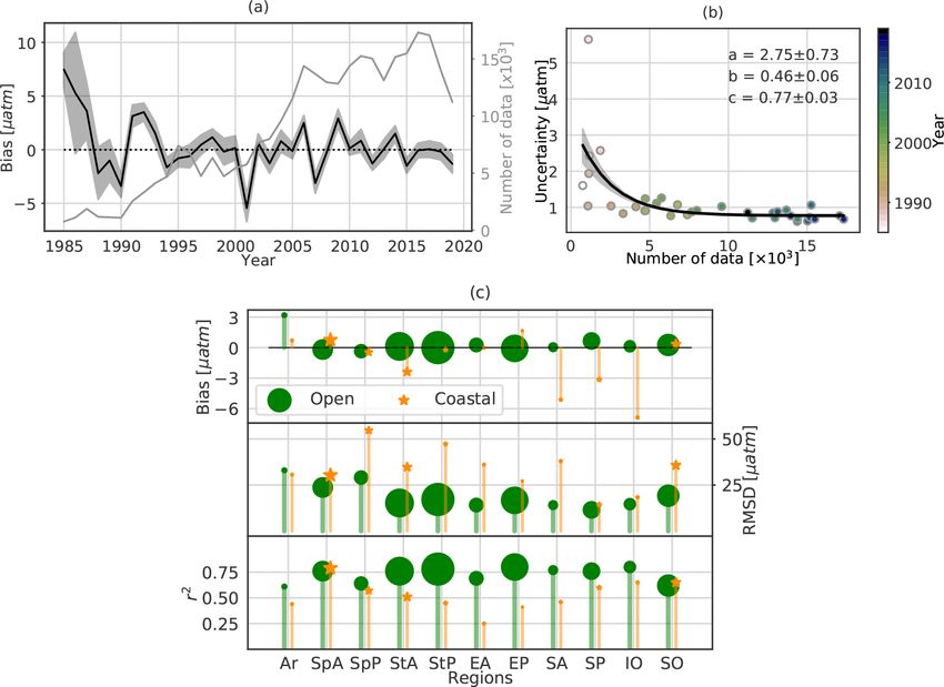
T. T. T. Chau et al.: pCO2 and air–sea CO2 flux estimates                                                                         1091

                                                                        Generally, RMSD measures the reconstruction skill in
                                                                     terms of the mean distance between model estimates and
                                                                     evaluation data, while r 2 measures the proportion of data
                                                                     variation predicted by the model. Compared to other met-
                                                                     rics such as mean absolute bias and r 2 , the RMSD takes
                                                                     another role, an outlier detector, which gives larger weights
                                                                     to high model–data misfits. Note that r 2 , µmisfit , σmisfit , and
                                                                     RMSD reflect the model performance with respect to evalua-
                                                                     tion data, while σensemble measures the stability of the model
                                                                     best estimate µensemble . Nevertheless, these different statis-
                                                                     tics should consistently reflect the skill of the model recon-
                                                                     struction, e.g. depending on the density and distribution of
                                                                     data sampling.
                                                                        In the next section, both the temporal and the spatial dis-
                                                                     tributions of gridded SOCAT data and in situ observations,
                                                                     model–data errors, model best estimates, and uncertainties
                                                                     are shown. An intensive analysis is presented for both the
                                                                     open-ocean and the coastal zones. We then interpret key
                                                                     factors leading to a good or poor reconstruction of surface
                                                                     pCO2 and fgCO2 , e.g. SOCAT data density and distribution,
Figure 2. Map of RECCAP1 regions (Regional Carbon Cycle As-          model design and resolution, regional to local characteristics
sessment and Processes; Canadell et al., 2011) and MARCATS           of pCO2 and fgCO2 , and their potential driving mechanisms.
(MARgins and CATchments Segmentation) coastal mask (Laruelle
et al., 2013) co-located on the 1◦ × 1◦ SOCAT grid.
                                                                     3     Results
          Reconstruction(i)
and pCO2                   is one of the 100 members of              3.1    Evaluation
the reconstructed pCO2      fields. Similar definitions are ap-
plied for fgCO2 . The units of air–sea flux estimates are            To verify the robustness of the mapping method, we first
molC m−2 yr−1 for a flux density, and this is converted to           evaluate the goodness of fit of reconstructed pCO2 against
PgC yr−1 for an integral over a region or the global ocean.          the independent SOCAT data from the leave-p-out cross-
   Model robustness of the reconstructed pCO2 fields is eval-        validation set (see Sect. 2.2).
uated on the gridded SOCAT data and in situ observations                Empirical cumulative distribution functions (CDFs) and
(Sutton et al., 2019). The evaluation data are denoted as            frequency histograms drawn from these data are compared
pCOObservation
     2          in the following formulas. Standard statistics       in Fig. 3a and b. While a frequency histogram in Fig. 3a
include the coefficient of determination (r 2 ); misfit mean         shows the number of gridded SOCAT pCO2 data distributed
(model bias) and misfit standard deviation,                          for each bin, the one in Fig. 3b (grey) reflects how the pCO2
            jP
             =N
                                                                     values in observational grid boxes are distributed within their
                        j                                            bounds. The probability–probability (P–P) plot of Fig. 3b
                   dpCO2
            j =1                                                     (blue curve) measures the fit in the distributions of the recon-
µmisfit =              ,
                 N                                                   struction and SOCAT data. The same presentation is used in
            v
            u j =N                 2                               Fig. 3c and d for the misfit standard deviation σmisfit and the
            u P          j                                           ensemble standard deviation σensemble (see their definitions in
            u       dpCO2 − µmisfit
            t j =1                                                   Eqs. 2 and 3 and their values in Fig. S3c and g).
σmisfit =                                ;                    (3)
                            N                                           The reconstructed pCO2 field matches SOCAT data
                                                                     well: both are normally distributed with the same mean of
and the root-mean-square deviation (RMSD),
                                                                     361.3 µatm (Fig. 3a), and a high agreement for all percentiles
                                                                     (Fig. 3b) is seen. The slight under- or overestimation at high
          v
          u j =N
                        j 2
          u P
          u       dpCO2                                              and low percentiles implies that the model is slightly biased
          t j =1
RMSD =                      ,                                 (4)    towards the mean value, as is expected when predictor vari-
                   N                                                 ables do not fully explain predictand variables in the training
                    j                                                dataset. This reduced variability is also reflected in the differ-
where dpCO2 = pCOReconstruction
                            2           (j ) − pCOObservation
                                                  2           (j )   ence between the data standard deviation based on SOCAT
and N is a number of evaluation data. All these scores are           pCO2 (41.79 µatm) and the one based on CMEMS-LSCE-
computed for different coastal and open regions from the             FFNN (36.30 µatm).
scale of grid cells to the global scale.

https://doi.org/10.5194/bg-19-1087-2022                                                      Biogeosciences, 19, 1087–1109, 2022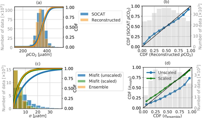
1092                                                                     T. T. T. Chau et al.: pCO2 and air–sea CO2 flux estimates

Figure 3. Comparison between empirical cumulative distribution functions (CDFs) of (a, b) SOCATv2020 data and the reconstructed pCO2
field and (c, d) model–data misfit standard deviation (σmisfit ) and model uncertainty (σensemble ), as seen in Fig. S3. In (c) and (d), the
distribution of σmisfit values scaled with a factor of 2 is plotted. A histogram with the axis in grey of the four subplots displays the number
of gridded data distributed in each bin; the bins with fewer than 200 data for (a) and 20 data for (c) have been excluded. In (b) and (d), the
bisector is shown in black.

   Displayed in Fig. 3c, both misfit standard deviation                     2. systematic errors between SOCAT data and the recon-
(σmisfit ) and model uncertainty (σensemble ) empirically fol-                 structed data equal those between the true data and the
low the exponential distribution. σmisfit is much higher than                  reconstructed data.
σensemble as the CDF and frequency histogram of the former
(blue) show heavier tails than those of the latter (orange),              As observation errors are independent from the random er-
which brings the P–P curve below the bisector in Fig. 3d.                 rors induced by the ensemble approach in each grid cell
When dividing the misfit standard deviation values shown                  (further to the implementation of the leave-p-out cross-
in Fig. S3c by 2, σmisfit (green) shares a similar distribution           validation in model training; see Sect. 2.2), σmisfit in Eq. (3)
to σensemble (orange). A natural explanation for this 2-fold              can be interpreted as
tuning factor would point to a simple lack of spread of the                2         2           2
                                                                          σmisfit = σensemble + σobservation ,                             (5)
ensemble, either because the FFNN ensemble would be too
small or because the uncertainty in the predictors (not ac-                        2
                                                                          where σobservation varies in space and time and is larger near
counted for here in the ensemble) would be significant. The               shelves (see the observation variability in Fig. S1b and c).
SOCAT CO2 fugacity data are sampled at an uneven space–                      The interpretation of the magnitude of mismatch is there-
time resolution (e.g. the sampling frequency varies between               fore not straightforward, but we note that the spatial distribu-
one read per minute to one per hour). Gridded data corre-                 tion of model errors and uncertainty estimates over the global
spond to the average of measurements collected within a                   ocean (Fig. 5) consistently identifies the spatial distribution
1◦ × 1◦ box and in a month over the entire cell area. Vari-               of the model skill. This asset is prioritized in our preliminary
ability in the sampling time and location of cruises and in-              study and further analysed in the next sections. The 2-fold
struments induces temporal sampling bias (e.g. towards some               factor used for the illustration in Fig. 3 has not been kept for
days in a month and/or the summer months at high latitudes)               the following results.
and latitude and longitude offsets from the cell centre (e.g.
with an average of 0.34◦ ± 0.14◦ as reported in Sabine et al.,            3.1.1   Global ocean
2013), which are not taken into account.
   Assume that                                                            At the global scale, the model fits the data with a mean
                                                                          bias close to zero, an RMSD of 20.48 µatm, and a coeffi-
  1. such practical imperfection presents a systematic error              cient of determination (r 2 ) of 0.76. The temporal fluctua-
     in each measurement from the true data with an overall               tion of the spatial mean of the model–data mean difference
     standard deviation of σobservation and                               over the global ocean is displayed in Fig. 4a along with the
                                                                          number of available gridded data. The time series of the
                                                                          yearly bias (black curve) starts with a large positive value

Biogeosciences, 19, 1087–1109, 2022                                                           https://doi.org/10.5194/bg-19-1087-2022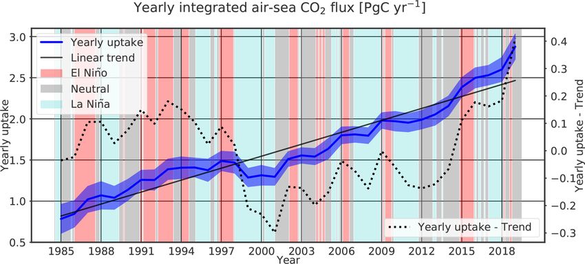
T. T. T. Chau et al.: pCO2 and air–sea CO2 flux estimates                                                                 1093

(7.47 ± 1.60 µatm) in the year 1985 (∼ 740 gridded data).         differences in characteristics and numbers of evaluation data
The bias drops during the following years and fluctuates          of pCO2 . In addition, the CMEMS-LSCE-FFNN model was
around zero from 1994 onwards (the number of grid boxes           designed with the leave-p-out cross-validation approach
containing SOCAT observations per year is generally larger        excluding many more independent data from monthly
than 5000). In general, the magnitudes of the yearly model        model fitting for model evaluation than the previous models.
bias and model spread are correlated with the number of           Overall model errors remain high despite the increase in the
observation-based data, which has increased greatly since the     spatial resolution and in the number of observations. Coastal
1990s. The importance of sustained data coverage is empha-        and shelf seas are characterized by complex physical and bi-
sized by Fig. S4. It illustrates the fact that large model–data   ological dynamics leading to high variability at small scales.
mismatches are frequently associated with the interruption        For instance, pCO2 levels over the Californian shelf can
of voluntary observing ship (VOS) lines and thus with the         exceed 850 µatm, with a spatial gradient of pCO2 as large
tracking of CO2 fugacity over large regions. The larger bias      as 470 µatm over a distance of less than 0.5 km (Chavez
computed prior to the 1990s (Fig. 4a) might intuitively lead      et al., 2018; Feely et al., 2008). Clearly, further model
to the conclusion that model outputs are less reliable than       improvement is needed in order to capture such high spatial
those in the later periods. However, this global mean score is    and temporal variability in surface ocean pCO2 present in
influenced by the number and distribution of data, and conse-     observations (see also Bakker et al., 2016; Laruelle et al.,
quently the increased data density does not fully explain the     2017, and references therein).
reconstruction skill. For instance, even with a higher num-          In the following subsections, we present and discuss the
ber of observation-based data than that in the pre-1990s, the     reconstruction skills for different ocean regions, as well as
years 2001 and 2007 stand out with strong negative biases         for open-ocean and coastal domains (Fig. 4c). Complete re-
(−5.44 ± 1.26 and −3.12 ± 0.92 µatm, respectively). While         sults including the numbers of gridded data, RMSDs, and r 2
such a comparison between the global bias and the number of       for each region are summarized in Table S2.
data highlights the lack of a simple relationship between the
number of data and the skill of the mapping method, the en-       3.1.2    Ocean basins
semble spread (dark grey area) of model errors, representing
the spread of the annual mean of pCO2 estimates on the SO-        Arctic
CAT grid with observations, is reduced with an exponential
decay constant of 0.46±0.06 per 1000 gridded data (Fig. 4b).      Data coverage is particularly sparse over the Arctic Ocean
   The model scores for the open ocean over the period 1985       (Ar) with 50 to 220 grid boxes with observations per year
to 2019 are 17.87 µatm for the RMSD and 0.78 for r 2 . The        since 2007 and an interruption in 2010 (Fig. S4). While con-
skill of this novel method, which uses only two-thirds of SO-     tinental shelves account for 50 % of the region’s area, only
CAT data for fitting each of 100 FFNN models, ranks sim-          one-third of the observation-based data are from coastal re-
ilarly to those from alternative statistical reconstruction ap-   gions. Moreover, observations are seasonally biased towards
proaches (Rödenbeck et al., 2013; Landschützer et al., 2014;      ice-free summer months (Bakker et al., 2016). Though re-
Gregor et al., 2019) which have been used to complement           construction standard errors are similar for open basins and
model-based estimates of the ocean carbon sink (Friedling-        coastal regions (RMSDs of 33.01 and 30.65 µatm, respec-
stein et al., 2019, 2020).                                        tively), the coefficient of determination is higher over the
   The CMEMS-LSCE-FFNN reconstruction over the                    open ocean (r 2 = 0.61) compared to coastal seas (r 2 = 0.44),
coastal regions for the full period is roughly 2 times less       suggesting a higher model skill over open basins. The close-
effective than over the open ocean in terms of the RMSD           to-zero bias of the coastal reconstruction shown in Fig. 4c
(35.86 µatm), while it shows a rather good fit with r 2 = 0.70.   results from the compensation between highly positive and
The high RMSD reflects high local model errors along the          negative values over the continental shelves of Alaska, the
continental shelves (Fig. S3). For the 1998–2015 period,          Canadian archipelagos, and the Barents and Kara seas (see
the CMEMS-LSCE-FFNN approach scored an RMSD                       Fig. S3); the yearly bias fluctuates within [−50, 30] µatm
of 35.84 µatm while a recent coastal reconstruction by            (Fig. S4). Of all open-ocean regions, the Arctic reconstruc-
Landschützer et al. (2020) obtained an error of 26.8 µatm         tion has the highest bias (3.19 µatm). Cold Arctic waters are
(see their Table 1). The latter presents a global ocean           characterized by low levels of surface ocean pCO2 due to the
pCO2 climatology product by unifying data over the same           temperature effect on CO2 solubility and the seasonal draw-
period from two conceptually equivalent reconstruction            down of dissolved inorganic carbon (DIC) during summer
models: one covering the open ocean at a 1◦ × 1◦ resolution       months by intense biological production (Feely et al., 2001;
(Landschützer et al., 2016) and one targeting the coastal         Takahashi et al., 2009; Arrigo et al., 2010). Assuming that
ocean at a 0.25◦ × 0.25◦ resolution (Laruelle et al., 2017).      the Arctic predictors remain within the range of global re-
These previous reconstructions cover the coastal region with      lationships, the overestimation of pCO2 by CMEMS-LSCE-
a broader definition (400 km distance from the seashore)          FFNN, as seen in Fig. 4c, suggests a possible underestima-
than the MARCATS mask used in this study, leading to the          tion of biological productivity. While this remains conjec-

https://doi.org/10.5194/bg-19-1087-2022                                                   Biogeosciences, 19, 1087–1109, 2022
1094                                                                    T. T. T. Chau et al.: pCO2 and air–sea CO2 flux estimates

Figure 4. (a) Time series of the yearly mean model bias, i.e. the reconstructed pCO2 data minus SOCATv2020 data, over the global ocean.
The black curve and dark grey area represent the mean estimate and 1σ envelope of errors of the 100-member ensemble; the light grey curve
represents the total number of gridded SOCAT data used in the FFNN model construction. (b) Exponential fits of the model uncertainty (the
magnitude of the 1σ envelope in Fig. 4a) against the number of gridded data per year. The exponential function is y = aexp−bx +c. The black
curve is derived from the best fit, and the grey-shaded area corresponds to the spread derived from standard errors of parameter estimates.
(c) Statistical scores for 11 oceanic regions with the size of each scattered object proportional to the number of regional data (Table S2).

tural, we acknowledge a large uncertainty in the contribution           scores, identify the Atlantic as the basin with the highest re-
of biological activity (net primary production, NPP) to sur-            construction skill. RMSDs corresponding to the StA, the EA,
face ocean pCO2 , as it is “proxied” by chlorophyll a derived           and the SA are below 15.50 µatm, and r 2 values are in the
from remote sensing (Maritorena et al., 2010; Babin et al.,             range of [0.69, 0.77]. While a larger RMSD is obtained over
2015). Overall, these scores point to the Arctic as a relatively        the SpA (23.68 µatm), the r 2 of 0.76 falls close to the upper
poorly reconstructed region.                                            end of the range determined for the three other regions. As
                                                                        discussed in Schuster et al. (2013), large temporal and spa-
Atlantic                                                                tial gradients of pCO2 as well as its variability driven by a
                                                                        diversity of physical and biological processes (e.g. surface
The North Atlantic stands out as a region with high data cov-           ocean temperature gradients, biological production, vertical
erage (Fig. S1a) and a rapidly increasing number of data                mixing, and horizontal advection of water masses) keep the
since 2000 (Fig. S4). A sustained sampling effort adds be-              analysis of pCO2 over the SpA challenging.
tween 2000 and 4000 data each year to the database over the                Despite accounting for over 59 % of the total coastal data,
Subtropical Atlantic (StA) and Subpolar Atlantic (SpA) re-              skilful data reconstruction over the coastal Atlantic regions
gions (including between 10 %–40 % of coastal data). The                remains difficult. RMSDs are in general above 30 µatm, and,
data density over the North Atlantic stands in strong contrast          with the exception of the coastal SpA (r 2 = 0.79), below
to the often fewer than 1000 gridded data per year collected            51 % of the observed variance is predicted by the model over
over the Equatorial Atlantic (EA) and South Atlantic (SA)               the other regions (StA, 0.51; EA, 0.25; SA, 0.46). The large
and their strong year-to-year variability.                              model–data mismatch along the Atlantic continental shelves
   The comparison between the reconstructed open-ocean                  (Fig. S3) reflects the poor reconstruction of pCO2 over re-
pCO2 and evaluation data over the four sub-regions of the               gions under the influence of upwelling systems (e.g. Moroc-
open Atlantic (Fig. 4c and Table S2) reveals small mean                 can coast, Benguela), large river discharges (e.g. Amazon,
model–data differences, which together with the two other

Biogeosciences, 19, 1087–1109, 2022                                                         https://doi.org/10.5194/bg-19-1087-2022
T. T. T. Chau et al.: pCO2 and air–sea CO2 flux estimates 1095
Congo, Florida, Mississippi), and the bottlenecks of gulfs or Niño years, e.g. 1986–1987, 1991–1992, 1997–1998) (see
bays (e.g. Bahamas, English Channel). the ENSO events highlighted in Fig. 9). A strong negative
bias is again computed in 2010–2012, which could reflect
Pacific the lack of data during that cooling phase. On the con-
trary, the reconstruction seems less sensitive to the strong
With the exception of the Subpolar Pacific (SpP), the number warm anomalies associated with the 2015–2016 El Niño. The
of observations has increased regularly over the Pacific basin. model appears to be more efficient at reconstructing surface
In recent years, there are from 1000 to 3500 grid boxes with ocean pCO2 during the hot climate mode (El Niño) than dur-
observations recorded over the Subtropical Pacific (StP), the ing the cool one (La Niña) when enhanced upwelling drives
Equatorial Pacific (EP), and the South Pacific (SP) (Fig. S4). surface ocean pCO2 up and towards unusually large val-
Forty percent of total open-ocean data belong to the StP and ues. This allows us to anticipate the effect of a general de-
the EP in the years 1985–2019. Corresponding RMSDs are crease in data collection and processing since 2020 in re-
17.15 and 16.68 µatm, with r 2 above 0.78. Despite a data sponse to the 2019 coronavirus disease (COVID-19) pan-
coverage below one-third of that reported for the two previ- demic on the estimation of the ocean carbon sink. We ex-
ous regions, the model proved skilful in reconstructing pCO2 pect a high negative bias in model estimates of pCO2 and
over the SP (Fig. 4c) with an RMSD of 11.50 µatm and r 2 the consequent underestimation of CO2 outgassing due to the
of 0.76. combined impact of data decreasing and La Niña conditions
The overall good performance of the FFNN over these governing since August and September 2020 (https://public.
three Pacific sub-regions contrasts with its lack of skill over wmo.int/en/media/press-release/la-nina-has-developed, last
the open SpP. The data density is poor and highly variable. access: December 2020). It is worthwhile to also note that
From before 1994, fewer than 250 gridded data per year are monthly gridded SOCAT data in the eastern EP have declined
available to constrain the reconstruction, followed by sev- in the last 5 years compared to the other years in the 2010s.
eral years of intense effort and a maximum of about 1250
data in 2000 before decreasing again to the pre-1994 values. Indian Ocean
At first order, skill scores fluctuate in line with data density.
During the first period (up to 1994), the bias varies within The Indian Ocean (IO) is the third-largest oceanic region by
[−25, 25] µatm (Fig. S4); it decreases close to [−2, 4] µatm area but also the one with the lowest data density. With the
between 1997 and 2000 and increases again along with de- exception of the year 1995 (approximately 1900 grid boxes
creasing data density. Much like the SpA, the SpP is a region including observations), as few as 500 gridded data have
characterized by a strong spatial and temporal variability been provided per year (Fig. S4), yielding a total number of
in pCO2 (Ishii et al., 2014), challenging any reconstruction data often below 10 per grid cell for the entire reconstruction
method. The difficulty is further aggravated by the paucity period (Fig. S1a). There have been even fewer than 75 grid
of data in this region compared to the SpA. Skill scores are boxes with observations per year over the continental shelf.
modest over the SpP with an RMSD of 29.08 µatm and r 2 of However, the reconstruction over the coastal region is com-
0.64 (Fig. 4c and Table S2). parable to the open IO with a low RMSD (< 19 µatm) and a
The ratio between coastal and open-ocean observation- high correlation with the observation-based data (r 2 = 0.65).
based data is 1 : 24. The paucity of data for the coastal The overall negative bias shown in Fig. 4c for the coastal
domain is reflected by lower skill scores compared to the IO points to the model underestimating coastal pCO2 levels.
open ocean. Over the coastal SpP, for example, the RMSD Large errors are distributed along the western Arabian Sea,
amounts to 54.69 µatm, while it is 29.08 µatm for the cor- western Madagascar, and the tropical eastern IO (Fig. S3).
responding open-ocean region. Comparable to the SpP, data These regions are under the influence of the southwest mon-
reconstruction over the coastal regions of the StP (e.g. North soon, giving rise to a seasonal upwelling regime (see Feely
American coast, Sea of Japan), as well as over the western EP et al., 2001; Sabine et al., 2002; Sarma et al., 2013, and refer-
(e.g. Peruvian upwelling) and the SP (e.g. offshore Chile), re- ences therein). Strong seasonal upwelling results in a marked
mains difficult (Fig. S3). Similar results have been found by seasonal cycle of surface ocean pCO2 with high levels during
Landschützer et al. (2020). the upwelling season. The paucity of data is likely to limit the
The EP is characterized by strong equatorial upwelling, skill of the model reconstruction of the seasonal cycle over
making it one of the major outgassing regions of CO2 (Feely large parts of the IO with consequences for the annual mean
et al., 2001). Surface ocean pCO2 shows a strong interan- analysed here.
nual variability predominantly in response to the El Niño–
Southern Oscillation (ENSO), the dominant regional cli- Southern Ocean
mate mode (Rödenbeck et al., 2015; Landschützer et al.,
2016; Denvil-Sommer et al., 2019). Before the 2000s, neg- Until recently, data coverage over the Southern Ocean (SO)
ative (positive) peaks of bias (Fig. S4) coincide with La was sparse (Fig. S1a), irregular at the grid cell scale, and bi-
Niña years, e.g. 1988–1990, 1995–1996, 1999–2001 (El ased towards austral summer months (e.g. Bushinsky et al.,
https://doi.org/10.5194/bg-19-1087-2022 Biogeosciences, 19, 1087–1109, 20221096 T. T. T. Chau et al.: pCO2 and air–sea CO2 flux estimates
2019; Gregor et al., 2019). A strong sampling effort allowed 0.84; SOFS, 0.79; TAO110W, 0.75; WHOTS, 0.73). Mean
a recent increase in observations to reach up to 2000 grid- bias µmisfit (Eq. 3) and the RMSD (Eq. 4) are relatively low
ded data per year (Fig. S4). Model scores for the open and compared to mean pCO2 values of the time series stations.
the coastal ocean are RMSDs of 19.18 µatm and 35.73 µatm, Half of the open-ocean reconstructions have model errors
respectively, and r 2 values of 0.62 and 0.65, respectively. of less than 20 µatm and are even less than 10 µatm at KEO,
The reconstruction lacks skill over the continental shelves of PAPA, SOLS, STRATUS, and WHOTS (Figs. S6 and S7).
South America and Antarctica (see Fig. S3). Despite having less skill than the open-ocean reconstruc-
In general, the pCO2 reconstruction over the SO has less tions, the coastal-ocean reconstructions are quite compatible
skill compared to the Atlantic or the Pacific due to the paucity with the in situ data (Fig. S8). Most of the RMSDs remain
of observation-based data compared to its large area. Röden- lower than 20 % of the mean pCO2 values of coastal time
beck et al. (2015) reported inconsistent reconstructed interan- series (e.g. CCE2, 36.53 µatm; ICELAND, 12.26 µatm; M2,
nual variability in pCO2 between different data-based meth- 36.58 µatm). For some other stations on the US west coast
ods. The interannual variability is large due to the natural and in the oceanic regimes of coral reef, the estimates differ
variability in the coupled ocean–atmosphere system charac- from the observation-based data in terms of the magnitude
terized by one of the globe’s strongest ocean currents, strong of pCO2 (e.g. CRIMP2, LA PARGUERA) and/or of its sea-
winds, and vertical mixing and upwelling of DIC-rich deep sonal cycle (e.g. CHABA, CHEECAROCKS, SEAK).
waters (Gregor et al., 2018; Gruber et al., 2019). Efforts The reconstructed time series cover the full period 1985–
to improve pCO2 reconstruction are ongoing and include 2019, while observation-based data are still sparse and al-
model development (e.g. Gregor et al., 2017), as well as the most all distributed over the past 2 decades (Figs. S6–S8).
increase in data coverage by the addition of data from differ- The CMEMS-LSCE-FFNN time series would be useful for
ent sampling platforms (e.g. profiling floats; Bushinsky et al., estimating and assessing long-term means, trends, and vari-
2019). For the time being, CMEMS-LSCE-FFNN stands out ations in CO2 surface partial pressure and the corresponding
as one of the skilful models with respect to observation- air–sea fluxes.
based data in the SO (Friedlingstein et al., 2020; Hauck et al.,
2020). 3.2 Long-term mean and uncertainty estimates
3.1.3 Time series stations Figure 5 shows temporal mean estimates, their associated un-
certainty, and RMSDs of the monthly air–sea pCO2 gradi-
CMEMS-FFNN-LSCE estimates of pCO2 are now com- ent (1pCO2 ) and CO2 fluxes (fgCO2 ) over the full period
pared with moored pCO2 time series provided by Sutton (see also Fig. S9 for the coastal regions only). On the top
et al. (2019). This data product comprises pCO2 measure- maps, the regions in blue are dominant CO2 uptake regions
ments collected from a wide range of oceanic regions since (influxes) and the regions in red are dominant source re-
2004 (Figs. S5–S8). Most of the stations were established gions of CO2 to the atmosphere (effluxes). The uncertainty
in the North Atlantic and the North Pacific and Equatorial in 1pCO2 is merely computed from the ensemble of the re-
Pacific; one site is in the IO and another in the SO. Approx- constructed sea surface pCO2 since the randomness in the
imately one-third of the Sutton et al. (2019) sites belong to atmospheric pCO2 field is assumed to be negligible. Due to
the coastal seas and shelves (Fig. S8). Table S3 details the impacts of wind stress, the solubility of CO2 , and seasonal
information of the moored pCO2 time series. sea-ice coverage on the gas transfer coefficient, spatial dis-
Observation-based data used for model–data compari- tributions of mean estimates, their uncertainty, and RMSDs
son (black points in Figs. S6–S8) are monthly averages of of 1pCO2 (Fig. 5a, c, e) and fgCO2 (Fig. 5b, d, f) differ
pCO2 measurements at each site. This interpolation results from low to high values. The means of air–sea fluxes inte-
in monthly time series with a number of data N between grated/averaged over different RECCAP1 regions (Table 1)
9 (NH10) and 98 (WHOTS). The ensemble mean µensemble are shown in Fig. 6. The distribution of uncertainty estimates
and ensemble spread σensemble (Eq. 2) are computed from and numbers of gridded SOCAT data for these regions are
the CMEMS-LSCE-FFNN ensemble of model outputs at the also displayed in Fig. 7, wherein only values smaller than the
four nearest model grid boxes of each location. Results con- 90 % quantile of uncertainty estimates shown in Fig. 5c and
firm a reasonably good reconstruction of the proposed ap- d are plotted to reduce the effects of outliers on data visual-
proach. The model best estimates (thick coloured lines) char- ization. The seasonal average computed over the full recon-
acterize pCO2 trends and variations in in situ data well, and struction period of air–sea CO2 fluxes over the global ocean
the model ensembles almost catch the observation-based data is shown in Fig. 8.
in their 99 % confidence interval (light shaded envelope).
For over 90 % of the time series stations, the model esti-
mation obtains a moderate to high coefficient of determi-
nation r 2 with a linear model–data correlation r larger than
0.5 (e.g. BTM, 0.98; CRESCENTREEF, 0.92; HOGREEF,
Biogeosciences, 19, 1087–1109, 2022 https://doi.org/10.5194/bg-19-1087-2022T. T. T. Chau et al.: pCO2 and air–sea CO2 flux estimates 1097
Table 2. Yearly mean of contemporary air–sea CO2 fluxes (PgC yr−1 ) integrated over the global ocean and 11 RECCAP1 regions. The mean
estimate and uncertainty (µensemble ± σensemble ) of the CMEMS-LSCE-FFNN approach is shown for the coast (C), the open ocean (O),
and the total area (T). For a comparison, estimates derived from RECCAP1 (Canadell et al., 2011; Schuster et al., 2013; Ishii et al., 2014;
Sarma et al., 2013; Lenton et al., 2013; Wanninkhof et al., 2013) are provided. In column “RECCAP1”, values in parentheses are the “best”
estimates proposed by RECCAP1 studies which were derived from averages or medians of estimates based on the pCO2 climatology or
pCO2 diagnostic model and/or the atmospheric and ocean inversions and GOBMs. The RECCAP1 values outside of parentheses are the
estimates derived from different methods mapping observation-based data of pCO2 . With an exception for the global estimate (denoted by ∗ )
(Wanninkhof et al., 2013), those of the RECCAP1 sub-basins are available only for the open ocean.
Approach CMEMS-LSCE-FFNN RECCAP1
Regions 1985–2019 1990–2009
Globe (T) 1.643 ± 0.125 1.486 ± 0.114
(O) 1.493 ± 0.122 1.344 ± 0.111 1.18∗
(C) 0.150 ± 0.010 0.141 ± 0.009 0.18∗
Arctic (Ar) (T) 0.027 ± 0.001 0.024 ± 0.001 (0.12 ± 0.06)
(O) 0.016 ± 0.001 0.015 ± 0.001
(C) 0.011 ± 0.001 0.010 ± 0.001
Subpolar Atlantic (SpA) (T) 0.259 ± 0.011 0.255 ± 0.010 0.07 ± 0.04, 0.30 ± 0.13
(O) 0.202 ± 0.009 0.197 ± 0.008 (0.21 ± 0.06)
(C) 0.057 ± 0.004 0.058 ± 0.004
Subtropical Atlantic (StA) (T) 0.214 ± 0.011 0.202 ± 0.009 0.18 ± 0.09, 0.24 ± 0.16
(O) 0.204 ± 0.010 0.192 ± 0.009 (0.26 ± 0.06)
(C) 0.010 ± 0.001 0.010 ± 0.001
Equatorial Atlantic (EA) (T) −0.117 ± 0.009 −0.128 ± 0.008 −0.10 ± 0.05, −0.12 ± 0.14
(O) −0.113 ± 0.009 −0.123 ± 0.008 (−0.12 ± 0.04)
(C) −0.004 ± 0.001 −0.004 ± 0.001
South Atlantic (SA) (T) 0.192 ± 0.016 0.174 ± 0.015 0.25 ± 0.12, 0.21 ± 0.23
(O) 0.184 ± 0.015 0.167 ± 0.015 (0.14 ± 0.04)
(C) 0.008 ± 0.001 0.007 ± 0.001
Subpolar Pacific (SpP) (T) 0.040 ± 0.010 0.029 ± 0.009 0.44 ± 0.21, 0.37
(O) 0.008 ± 0.008 −0.002 ± 0.007 (0.47 ± 0.13)
(C) 0.032 ± 0.004 0.031 ± 0.003
Subtropical Pacific (StP) (T) 0.523 ± 0.016 0.512 ± 0.014
(O) 0.495 ± 0.015 0.485 ± 0.014
(C) 0.028 ± 0.003 0.027 ± 0.002
Equatorial Pacific (EP) (T) −0.503 ± 0.022 −0.514 ± 0.020 −0.51 ± 0.24, −0.27
(O) −0.490 ± 0.021 −0.500 ± 0.020 (−0.44 ± 0.14)
(C) −0.013 ± 0.003 −0.013 ± 0.003
South Pacific (SP) (T) 0.358 ± 0.029 0.343 ± 0.029 0.29 ± 0.14, 0.24
(O) 0.352 ± 0.029 0.337 ± 0.028 (0.37 ± 0.08)
(C) 0.006 ± 0.0004 0.006 ± 0.0004
Indian Ocean (IO) (T) 0.300 ± 0.033 0.281 ± 0.027 0.24 ± 0.12
(O) 0.305 ± 0.033 0.286 ± 0.027 (0.37 ± 0.06)
(C) −0.004 ± 0.002 −0.005 ± 0.002
Southern Ocean (SO) (T) 0.349 ± 0.070 0.307 ± 0.061 0.27 ± 0.13
(O) 0.330 ± 0.069 0.290 ± 0.061 (0.42 ± 0.07)
(C) 0.018 ± 0.002 0.017 ± 0.002
https://doi.org/10.5194/bg-19-1087-2022 Biogeosciences, 19, 1087–1109, 20221098 T. T. T. Chau et al.: pCO2 and air–sea CO2 flux estimates
Figure 5. Climatological mean (a, b) and uncertainty (c, d) of air–sea pCO2 difference (a, c) and of CO2 fluxes (b, d) over 1985–2019.
Uncertainty (Eq. 2) is computed as the standard deviation of the 100-member CMEMS-LSCE-FFNN model outputs of sea surface pCO2
and air–sea CO2 fluxes. The bottom panels (e, f) show RMSDs (Eq. 4) between the SOCAT data (or data-based estimates of fluxes for f) and
the mean CMEMS-LSCE-FFNN model outputs.
Figure 6. Distribution of contemporary fluxes (positive into the ocean) over 11 regions (see in Fig. 2) for the full period 1985–2019.
Uncertainties in the mean estimates of air–sea fluxes integrated (a) or averaged (b) over each region are shown with error bars.
3.2.1 Arctic tors (e.g. the Norwegian Sea, the Barents Sea, the Kara Sea)
are CO2 sinks with moderate influx densities (Fig. 8). The
The Arctic Ocean stands out as the region with the strongest open-ocean influx density exceeds 3 molC m−2 yr−1 in the
CO2 uptake per unit area with 2.336 ± 0.104 molC m−2 yr−1 Arctic summer. This substantial amount of CO2 uptake is
for the open sea and 1.522 ± 0.108 molC m−2 yr−1 for the driven by low surface ocean temperature, seasonal changes
continental shelf margins (Figs. 5b and 6b). At the scale of in sea-ice cover, and intense biological production. Increas-
grid cells, air–sea gradients of pCO2 are large, but the down- ing light availability and input of nutrients through meltwa-
ward fluxes are relatively modest over the shelves of eastern ters and river discharges sustain high levels of primary pro-
Greenland, the Barents and Kara seas, and the Siberia seas duction and CO2 drawdown (Bates and Mathis, 2009; Arrigo
(Figs. 5 or S9). During the sea-ice-covered seasons, these et al., 2010; Yasunaka et al., 2016, 2018). Notwithstanding,
coastal regions are neutral while the open-ocean Arctic sec- the Arctic Ocean represents roughly 0.58 % of the total sur-
Biogeosciences, 19, 1087–1109, 2022 https://doi.org/10.5194/bg-19-1087-2022T. T. T. Chau et al.: pCO2 and air–sea CO2 flux estimates 1099
Figure 7. Distribution (violin) of all uncertainty estimates (Fig. 5c and d) and the total number (star) of gridded SOCAT data (Fig. S1a)
split for 11 RECCAP1 regions. A violin plot shows the range, median, and density of uncertainty estimates for pCO2 (µatm) and fgCO2
(molC m−2 yr−1 ).
Figure 8. Seasonality of downward CO2 fluxes (molC m−2 yr−1 ) in 1985–2019. Temporal means of the reconstructed fgCO2 field for
January to March (JFM), April to June (AMJ), July to September (JAS), and October to December (OND) are shown.
face ocean area (Table 1), and the yearly mean CO2 uptake (Fig. 6a). The interplay between temperature- and biology-
integrated over the Arctic for the full period amounts to only driven effects results in changes in the seasonal and spatial
1.64 % of the global ocean sink (Table 2 and Fig. 6a). distributions of surface ocean pCO2 and ultimately air–sea
CO2 fluxes. During boreal winter–spring, high wind speeds
3.2.2 Atlantic enhance gas transfer velocities and contribute to a strong
cooling and an increase in CO2 solubility (Takahashi et al.,
The open-ocean Subpolar Atlantic (SpA) sink contributes ap- 2009; Feely et al., 2001), both enhancing uptake of CO2 over
proximately 78 % to the total SpA annual C uptake (0.259 ± the Labrador Sea, the North Atlantic and Norwegian cur-
0.011 PgC yr−1 ), as well as 12.29 % to the total ocean rents, and the Barents and Kara seas (Fig. 8). High wind
sink (1.643 ± 0.125 PgC yr−1 , Table 2). Per unit area, the speeds also strengthen vertical mixing, a process supplying
open-ocean influx amounts to 2.012 ± 0.092 molC m−2 yr−1 dissolved inorganic carbon (DIC) and nutrients to the sur-
and the coastal-ocean influx is 30.51 % less than its open- face ocean. During the spring and summer months, vigor-
ocean counterpart and slightly lower than the coastal Arc- ous biological activity (Sigman and Hain, 2012) counter-
tic sink (Fig. 6b). However, when integrated over the re- acts the warming-induced decrease in CO2 solubility and in-
gion, the yearly uptake of 0.057 ± 0.004 PgC yr−1 makes the crease in pCO2 by drawing down DIC (Feely et al., 2001).
coastal SpA the strongest sink among the 11 coastal regions
https://doi.org/10.5194/bg-19-1087-2022 Biogeosciences, 19, 1087–1109, 2022You can also read