Attachment 7.3.1 Connections, Energy and Demand Forecast Methodology Access Arrangement Supplementary
←
→
Page content transcription
If your browser does not render page correctly, please read the page content below

Attachment 7.3.1
                       Connections, Energy and Demand
                       Forecast Methodology
                       Access Arrangement Supplementary
                       Confidential

                       2 October 2017

Access Arrangement Supplementary (AAS) for the period
1 July 2017 to 30 June 2022
Connections, Energy
and Demand Forecast
Methodology
Confidential
7 August 2017

                 EDM#34382992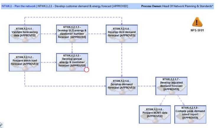
Western Power
363 Wellington Street
Perth WA 6000
GPO Box L921 Perth WA 6842

Document Information
Title              Connections, Energy and Demand Forecast Methodology

Subtitle           N/A

Authorisation
                   Title                           Name                              Date
Author             Forecasting & Modelling         Ben Jones                         19/07/2017
                   Team Leader

Reviewer           Insights & Analytics            Grant Coble-Neal                  27/07/2017
                   Management

Approver:          Head of Business Intel &        David Hebden                      07/08/2017
                   Data Analytics                                                    EDM 43327337

Document History
Rev      Date              EDM           Amended by               Details of amendment
No                         Version
   1     27/10/2016            12        Grant Coble-Neal         RCP1 preparation

   2     31/07/2017            16        Grant Coble-Neal         Updated alignment for AA4 submission

Review Details
Review Period:               2016/17

NEXT Review Due:             July 2018

                       Access Arrangement Supplementary for the fourth period (AAS)
                      Strictly confidential and commercially sensitive to Western Power     EDM#34382992
                                                                                                   Page ii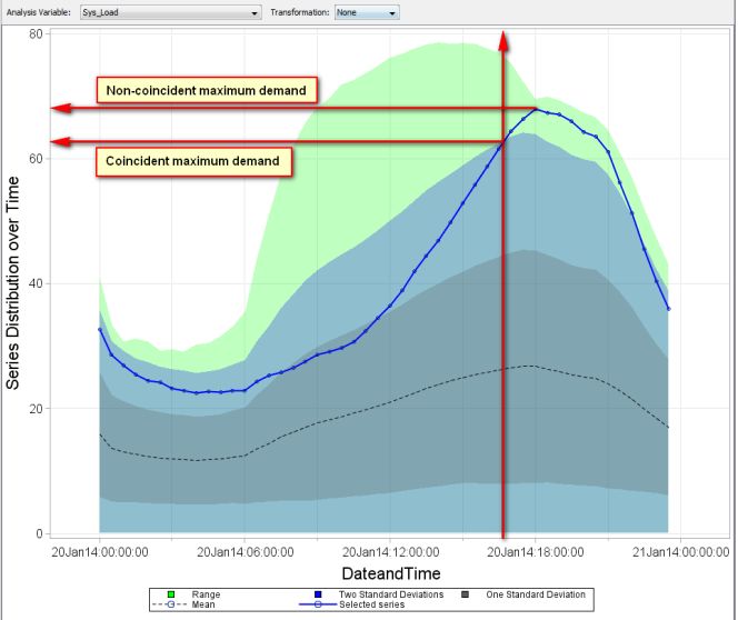
Contents

Glossary ...................................................................................................................................................... vi
Document References .................................................................................................................................. x
1.     Introduction .........................................................................................................................................1
       1.1        Purpose ..................................................................................................................................... 1
       1.2        Structure .................................................................................................................................... 1
2.     Forecasting process overview ..............................................................................................................2
       2.1        Purpose of producing forecasts .................................................................................................. 2
       2.2        Process description .................................................................................................................... 3
                  2.2.1          NTWK 1.2.1 Energy and Customer Demand Forecast .......................................... 3
                  2.2.2          Process steps.................................................................................................... 4
                  2.2.3          Supply zone classification system ...................................................................... 5
                  2.2.4          Forecast platforms............................................................................................ 5
3.     Forecasting principles...........................................................................................................................6
       3.1        Application of principles in practice ............................................................................................ 6
                  3.1.1          Accurate and unbiased...................................................................................... 6
                  3.1.2          Transparent and repeatable .............................................................................. 6
                  3.1.3          Evidence-based and data-driven ........................................................................ 7
4.     Data preparation ..................................................................................................................................8
       4.1        Extract and validate data ............................................................................................................ 8
       4.2        Tolerance for imperfection......................................................................................................... 9
       4.3        Root cause analysis .................................................................................................................. 10
       4.4        Data validation quality checking process .................................................................................. 11
5.     Overview of underlying load growth forecast methods ..................................................................... 12
       5.1        Introduction ............................................................................................................................. 12
       5.2        New connection forecasts ........................................................................................................ 12
       5.3        Energy per connection trend forecasts ..................................................................................... 13
       5.4        Composite trend forecasting .................................................................................................... 13
6.     Underlying load growth forecast model description .......................................................................... 14
       6.1        Time series statistics methods .................................................................................................. 14
       6.2        Econometric forecasts .............................................................................................................. 15
                  6.2.1          Benefits of employing reduced form models .................................................... 15

                                    Access Arrangement Supplementary for the fourth period (AAS)
                                  Strictly confidential and commercially sensitive to Western Power                                      EDM#34382992
                                                                                                                                               Page iii
6.2.2          Underlying drivers of electricity demand ......................................................... 15
7.     Maximum demand forecasts.............................................................................................................. 21
       7.1      Introduction ............................................................................................................................. 21
       7.2      Overview of the key steps ........................................................................................................ 22
       7.3      Scaling average demand to calculate maximum demand forecasts ........................................... 22
                7.3.1          Scaling by load factor ...................................................................................... 22
                7.3.2          Uncertainty bands .......................................................................................... 23
                7.3.3          Coincident and non-coincident demand ........................................................... 25
                7.3.4          Alternative maximum demand forecast model selection ................................... 26
8.     Forecasting assumptions .................................................................................................................... 28
       8.1      Introduction ............................................................................................................................. 28
       8.2      Medium term (five year) forecast assumptions ........................................................................ 28
       8.3      Long-term (six plus years) forecast assumptions....................................................................... 29
       8.4      Assumptions not explicitly incorporated in the long term forecasts .......................................... 29
9.     Block load forecasts ........................................................................................................................... 31
       9.1      Prepare block load forecasts .................................................................................................... 31
10. Forecast reporting .............................................................................................................................. 33

List of tables
Table 1: Energy and customer demand forecast delivery steps: .................................................................... 4

Table 2: External variable description ......................................................................................................... 16

Table 3: customer incentive modelling of customer supply scenarios .......................................................... 19
Table 4: External variables forecasts ........................................................................................................... 28

List of figures
Figure 1: Process overview............................................................................................................................ 3

Figure 2: Responsibilities for extracting and validating data .......................................................................... 8
Figure 3: Iterative loop process flow ............................................................................................................. 9

Figure 4: Wundowie (WUN) substation data from the validation process .................................................... 11

Figure 5: Technology Forecasts ................................................................................................................... 20
Figure 6: Simplified overview of the ‘end to end’ process used to develop the final forecasts ..................... 21

                                  Access Arrangement Supplementary for the fourth period (AAS)
                                Strictly confidential and commercially sensitive to Western Power                                    EDM#34382992
                                                                                                                                           Page iv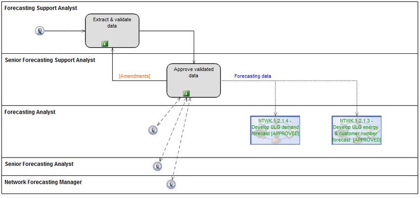
Figure 7: Load factor calculation example ................................................................................................... 23

Figure 8: Example of a maximum demand spike caused by a factor other than weather ............................. 24

Figure 9: Coincident versus non-coincident maximum demand ................................................................... 26
Figure 10: Block load evaluation criteria...................................................................................................... 32

                                 Access Arrangement Supplementary for the fourth period (AAS)
                               Strictly confidential and commercially sensitive to Western Power                            EDM#34382992
                                                                                                                                   Page v
Glossary
The following table provides a list of abbreviations and acronyms used throughout this document. Defined
terms are identified in this document by capitals.
Term Definition
ABS Australian Bureau of Statistics
Annual average demand Average electricity demand over the course of one year, usually expressed in
MW.
In this discussion, annual average demand refers to the annual average
measured at five minute intervals. This is equivalent to the average annual
volume of electricity consumed.
Annual peak demand or The highest average electricity consumption in any five minute interval during
Annual maximum the course of one year, usually expressed in MW.
demand
ARIMA Auto-regressive Integrated Moving Average
Augmented Dickey Fuller An augmented Dickey Fuller test (ADF) tests the null hypothesis of whether a
test unit root is present in a time series sample. The alternative hypothesis is
different depending on which version of the test is used, but is usually
stationarity or trend-stationarity.
BDP Binningup Desalination Plant
Block load If a customer’s requested demand is above the forecast underlying growth in
demand, then this is known as a block load. Once added to underlying demand
growth, a block load introduces an often permanent step-change into an
otherwise smooth trend.
BOM Bureau of Meteorology
Box plot A box plot, sometimes called a box and whisker plot, is a type of graph used to
display patterns of quantitative data.
CAGR Compound annual growth rate
CER Clean Energy Regulator
CO Customer-owned
Coefficient of variation The coefficient of variation (CV), also known as relative standard deviation
(RSD), is a standardised measure of dispersion of a probability distribution or
frequency distribution.
Coincident and non- See section 7.3.3 of this document for the definitions.
coincident demand
Access Arrangement Supplementary for the fourth period (AAS)
Strictly confidential and commercially sensitive to Western Power EDM#34382992
Page viTerm Definition
Cooling degree days Cooling degree days are a measure of how much (in degrees), and for how
long (in days), the outside air temperature was above a certain level. They are
commonly used in calculations relating to the energy consumption required to
cool buildings.
Cross-price elasticity The cross-price elasticity of demand measures the responsiveness of the
quantity demanded for a good to a change in the price of another good, all
other relevant factors remaining the same.
Diversity factor See section 7.3.4 of this document.
EVs Electric Vehicles
Heating degree days Heating degree days are a measure of how much (in degrees), and for how
long (in days), the outside air temperature was below a certain level. They are
commonly used in calculations relating to the energy consumption required to
heat buildings.
HIA Housing Industry Association
HVAC HVAC (heating, ventilating/ventilation, and air conditioning). Its goal is to
provide thermal comfort and acceptable indoor air quality.
kWh Kilowatt-hour. Is a basic measuring unit of electric energy equal to one
kilowatt of power supplied to or taken from an electric circuit steadily for one
hour. One kilowatt-hour equals 1,000 watt-hours. One kilowatt-hour can
power ten 100 watt light bulbs for one hour.
Load factor The ratio of annual average demand to annual peak demand.
This is a partial indicator of network utilisation.
MAPE Mean Absolute Percentage Error: For an actual vs forecast comparison the
absolute values of the percentage errors are summed and the average is
computed.
MBS data Metering Business System data that is associated with managing revenue
meters connected to the Western Power Network.
Multivariate regression Multivariate regression is a technique that estimates a single regression model
with more than one outcome variable.
MVA MVA stands for Mega Volt Amp or Volts X Amp /1,000,000. If the total load
requirement is 1,000 volts and 5,000 amps (1,000 x 5,000 = 5,000,000 VA) it
can be expressed as 5MVA. This is called "apparent power" because it takes
into consideration both the resistive load and reactive load.
MW Megawatt. One megawatt equals one million watts and is a measure of the
active component of electrical demand.
Access Arrangement Supplementary for the fourth period (AAS)
Strictly confidential and commercially sensitive to Western Power EDM#34382992
Page viiTerm Definition
MWh Megawatt-hour. Is a measure of electrical energy i.e. one megawatt-hour
equals one million watt-hours. For example, one MWh of electricity can
power ten thousand 100 watt light bulbs for one hour.
NetCIS data Data retrieved from NetCIS which is Western Power’s core customer care and
billing system. NetCIS stores most of the company’s customer information and
interactions and is used on a daily basis throughout the organisation. It is the
system used to calculate and invoice network access charges and bill these
charges to electricity retailers.
NMI NMI or the National Metering Identifier is a unique identifier that identifies a
supply or connection point and is assigned by the providing distributor.
Outliers Observations in a data set that are substantially different from the bulk of the
data. An outlier may be due to variability in the measurement or it may
indicate experimental error; the latter may be excluded from the data set.
PoE Probability of Exceedance: This is the percentage of time that an actual value is
expected to exceed the forecast value e.g. a PoE 10 forecast is expected to be
exceeded 10% of the time i.e. one year in ten. And a PoE 20 forecast is
expected to be exceeded 20% of the time i.e. one year in five.
Power factor Power factor is the ratio between the MW and the MVA drawn by an electrical
load where the MW is the actual load power and the MVA is the apparent load
power.
Predictor variable Is an independent variable that is manipulated in an experiment in order to
observe the effect on a dependent variable.
Regression analysis Regression analysis is a statistical modelling process for estimating the
relationships among variables. It includes many techniques for modelling and
analysing several variables, when the focus is on the relationship between a
dependent variable and one or more independent variables (or 'predictors').
SC Seasonal Component
SCADA data The SCADA (Supervisory Control and Data Acquisition) system is Western
Power's critical system for managing the electricity network, both day to day
and in emergencies. This network data is monitored and recorded.
Serial correlation Serial correlation is the relationship between a given variable and itself over
various time intervals. Serial correlations are often found in repeating
patterns, when the level of a variable effects its future level.
Sigmoid function A sigmoid function is a bounded differentiable real function that is defined for
all real input values and has a positive derivative at each point.
SMEs Subject Matter Experts
Access Arrangement Supplementary for the fourth period (AAS)
Strictly confidential and commercially sensitive to Western Power EDM#34382992
Page viiiTerm Definition
Standard deviation A common measure of spread in the distribution of a random variable.
Standard error of mean The standard error of mean (SEM) estimates the variability between sample
means that you would obtain if you took multiple samples from the same
population. The standard error of mean estimates the variability between
samples whereas the standard deviation measures the variability within a
single sample.
Summer Summer refers to the period 1 December to 31 March (inclusive).
SWIN South West Interconnected Network. Is all the transmission and distribution
components of the electricity system. And comprises the Western Power
Network and other transmission and distribution assets owned and operated
by others.
SWIS South West Interconnected System. Is the entire electricity system including all
of the generators. And comprises the Western Power Network, other
transmission and distribution assets owned and operated by others and all of
the generators.
Test of unit root or unit A 'unit root test' tests whether a time series variable is non-stationary and
root test possesses a unit root. The null hypothesis is generally defined as the presence
of a unit root and the alternative hypothesis is either stationarity, trend
stationarity or explosive root depending on the test used.
Time series A time series is a series of data points listed (or graphed) in time order. Most
commonly, a time series is a sequence taken at successive equally spaced
points in time. Thus it is a sequence of discrete-time data.
Topaz A Western Power database that is used to store and maintain up to date
information relating to customers' connection applications.
VAR Vector Auto-regressive
Weather correction In the context of demand, weather correction refers to the estimation of
maximum demand based on expected weather outcomes to create a weather-
normalised maximum demand series.
Western Power Network Is the transmission and distribution element of the SWIN that is owned and
operated by Western Power.
Winter Winter refers to the period 1 May to 31 August (inclusive).
WPN Western Power–owned
WUN Wundowie Substation
Access Arrangement Supplementary for the fourth period (AAS)
Strictly confidential and commercially sensitive to Western Power EDM#34382992
Page ixDocument References
Doc # Title of document
42747934 2017 Maximum demand forecasts (Summer) by zone substation
42774252 Energy & Customer Numbers Forecast - 2017
Access Arrangement Supplementary for the fourth period (AAS)
Strictly confidential and commercially sensitive to Western Power EDM#34382992
Page x1. Introduction
1.1 Purpose
This document describes the methodology used to prepare the following forecasts for the fourth access
arrangement period commencing 1 July 2017:
1. number of new connections
2. energy forecasts
3. maximum demand.
The scope of this document includes both transmission and distribution networks.
1.2 Structure
This document is organised as follows:
Section 2 provides an overview of Western Power’s forecasting process.
Section 3 briefly articulates the principles guiding key decisions made in constructing forecasts
Section 4 explains the data preparation process.
Section 5 provides a conceptual overview of the structure and organization of the underlying load
growth forecast.
Section 6 describes the methods used to forecast trend growth in underlying load caused by growth in
population, household formation and the economy.
Section 7 explains how the underlying load growth forecasts are used to create maximum demand
forecasts.
Section 8 summarises the key forecasting assumptions and indicates the sources of those
assumptions.
Section 9 provides an outline of the block load forecast method.
Section 10 lists the range of forecast reports subsequently produced.
Access Arrangement Supplementary for the fourth period (AAS)
Strictly confidential and commercially sensitive to Western Power EDM#34382992
Page 12. Forecasting process overview
Key messages:
As a Transmission and Distribution Network Service provider, Western Power produces and reconciles
new connection, energy and maximum demand forecasts at the whole of network level, by load area,
by zone substation area and by HV feeder area.
These forecasts are part of a wider set of forecasts, which extend to: solar photovoltaic power system
connections; electricity volume transported via the Western Power Network; and electricity volume
imported from distribution connected generation.
The forecasts are primarily bottom-up forecasts consisting of hundreds of forecasting models. The
primary benefit of forecasting at a detailed level is maximum flexibility and simplicity. That is,
relatively simple and largely data-driven models are fitted to specific customer segments (i.e.
Commercial, Industrial and Residential). Model coefficients are allowed to adjust across regions;
meaning that a given customer segment (e.g. residential customers) may contain coefficient estimates
that are statistically different across regions. In addition, responses to systematic seasonal variation
(e.g. in temperature, sunlight etc) is allowed to vary across forecast region.
The forecasts at zone substation level and above are a composite of many trends, the most important
being: new connection growth, amount of solar photovoltaic generation, response to variation in
electricity prices, and economic activity.
2.1 Purpose of producing forecasts
The Regulation and Investment Management and Finance Treasury and Risk functions require the
preparation of forecasting processes to assist with:
Review of the annual price list – Allows Western Power to forecast expected revenues, and adjust the
price list accordingly.
Budgeting – Allows Western Power to forecast maintenance requirements.
Network planning (capacity and reliability performance) – Allows Western Power to forecast growth
requirements.
The forecasts produced to assist with these objectives include:
number of customers/connections
metered energy sold to customers
maximum demand
network reliability performance.
In delivering these outcomes, Western Power follows defined processes described in the Process Library.
An overview of the forecasting process is illustrated in Figure 1 (next page).
Access Arrangement Supplementary for the fourth period (AAS)
Strictly confidential and commercially sensitive to Western Power EDM#34382992
Page 2Figure 1: Process overview
Western Power produces the required forecasts through process NTWK.1.2.1 ‘Energy and Customer
Forecast’. This process defines the validation of forecasting data, development of forecasts, and compiling
the reports.
Customer connections and energy forecasts are in accordance with process NTWK.1.2.1.5 ‘Energy and
Customer Forecast’. The process for determining the trends in peak demand and network reliability
performance outcomes is process NTWK.1.2.1.9 ‘Develop customer demand and energy forecast’.
Western Power produces forecasts as defined in Western Power’s Process Library. The role of these
defined processes is to ensure that the forecasts are produced in a predictable and transparent manner
that is fit-for-purpose for use in defined downstream processes, i.e. budgeting, pricing and planning.
2.2 Process description
2.2.1 NTWK 1.2.1 Energy and Customer Demand Forecast
This process delivers the energy (i.e. MWh) and maximum demand (MW) forecasts and consists of nine
process steps. The process culminates with the delivery of the:
Energy and Customer Numbers Forecast required by Strategy, Regulation and Finance for the Annual
Price Review and for quarterly budgeting.
Peak Demand Trend report, which presents peak demand forecasts by zone substation.
Network Capacity Mapping Tool update, which provides a public view of the available substation
capacity net of the forecast demand, excluding the impact of upstream transmission constraints that
limit the substation capacity actually available.
Access Arrangement Supplementary for the fourth period (AAS)
Strictly confidential and commercially sensitive to Western Power EDM#34382992
Page 32.2.2 Process steps
The process steps are explained in Table 1.
Table 1: Energy and customer demand forecast delivery steps
Process Process Name Process Description
Number
NTWK.1.2.1.1 Validate forecasting data Check the data (i.e. monthly kWh and customer
numbers, annual maximum demand data and external
variables) and ensure that it is suitable for developing
forecasts.
NTWK.1.2.1.2 Prepare block load forecasts Review prospective connection applications and
determine which connection applications impose a
step change in forecast trends. Apply the Block Load
Criteria to determine the magnitude and timing of the
connection applications deemed to be block loads.
NTWK.1.2.1.3 Develop underlying load growth Using the received and validated forecasting data,
energy and customer numbers apply appropriate forecast methods (e.g. times series
forecasts statistics) to forecast small customer numbers and
load. These are typically forecast as energy per active
NMI and number of active NMIs.
NTWK.1.2.1.4 Develop underlying load growth Calculate monthly GWh forecasts: product of energy
forecasts per active NMI and the number of active NMIs.
NTWK.1.2.1.5 Develop annual energy and Add the block load forecast to the underlying load
customer forecasts growth forecasts. Convert monthly GWh forecasts to
annual.
NTWK.1.2.1.6 Develop demand forecast Determine load factors by zone substation,
transmission load area, scale and convert the annual
GWh forecasts to maximum demand (measured in
MW).
NTWK.1.2.1.7 Develop adjusted demand Adjust the maximum demand forecasts to reflect any
forecast planned network reconfiguration.
NTWK.1.2.1.8 Prepare the Network Capacity Create a spatial layer using Geographical Information
Mapping Tool data System tools and present on the Network Capacity
Mapping Tool layer.
NTWK.1.2.1.9 Compile the peak demand trend Create a report, combining both quantitative and
report qualitative information.
Access Arrangement Supplementary for the fourth period (AAS)
Strictly confidential and commercially sensitive to Western Power EDM#34382992
Page 42.2.3 Supply zone classification system
There are many systematic differences in demand characteristics across supply zones, which requires
application of different forecast assumptions across supply zones. To facilitate the orderly management of
these differences, the supply areas are classified as follows:
Load area: each zone substation is assigned to one of 15 load areas as defined in the Annual Planning
Report, Appendix C.
Ownership: zone substations are either Customer-Owned (CO) or Western Power–Owned (WPN).
2.2.4 Forecast platforms
Western Power primarily relies on the SAS platforms Enterprise Guide and Forecast Studio for forecasting
purposes. The open source software R (by CRAN) is also used for parts of the forecast process. The primary
benefit of these platforms is that documentation is created as a by-product of forecasting which is
consistent with the principles of transparency and ability to replicate the forecast.
Enterprise Guide is a platform for creating scripted tasks via a ‘point and click’ interface or by direct coding.
These are organised into pre-forecast and post-forecast process flows. Use of Order Lists provide a means
of specifying the order of task implementation, ensuring that these processes are implemented in the same
way each time the process is executed.
Forecast Studio provides state-of-the-art machine generated forecasts, which can then be customised to
reflect knowledge about a given forecast that is not already reflected in the data. There are several
automatically generated forecasts that can be compared. Forecast Studio also provides a convenient means
of reconciling multi-level forecasts.
Figure 2: Illustration of forecast hierarchy for commercial customer numbers forecasts for commercial
customers
Tariff group level
Tariff sub-level
Tariff level
The primary benefit in multi-level forecasting is the ability to reconcile small area dynamics with tariff level
and network level demand profiles. This reduces forecast bias and consequently enhances accuracy while
maintaining insights with respect to the individual contribution of distinct trends such as population and
technology trends, which are typically identified in network and tariff level models.
R is an industry standard tool that provides specialist algorithms which are simple to implement and may in
some cases produce an easier to customise process. There are also packages in R, such as GGPLOT2, which
provides enhanced visualisation of data.
Access Arrangement Supplementary for the fourth period (AAS)
Strictly confidential and commercially sensitive to Western Power EDM#34382992
Page 53. Forecasting principles
Key messages:
Before engaging in the complexities of forecasting, it is important to establish principles to guide the
multitude of decisions that need to be made
Principles guide choices about how the forecasts are done, particularly where there are trade-offs in
outcome. For example, simplicity versus comprehensiveness, speed versus insight
The three primary principles applied by Western Power are accuracy, transparency and evidence-
based decisions
Western Power strives to deliver forecasts that are:
accurate and unbiased
transparent and repeatable
evidence-based and data-driven.
In doing so:
identify and incorporate key trend drivers
design, validate and test forecast models
ensure consistency of forecasts at different levels of aggregation
use the most recent input information available.
3.1 Application of principles in practice
3.1.1 Accurate and unbiased
Western Power monitors the accuracy of past forecasts, with a primary focus on the most recent forecasts,
by comparing actual data against the forecasted data. By continually adding actual data into the forecasting
processes the analysis becomes more accurate. Periodic forecast accuracy assessments are conducted with
a focus on:
monitoring the typical level of accuracy
understanding the causes of inaccuracy
Evidence of this practice is available in the Annual Planning Report.
Any evidence of bias is incorporated in adjustments made in the design of new forecast models, which
extends consideration to the type and quality of the data relied on to calibrate forecast models.
3.1.2 Transparent and repeatable
Western Power employs good practices, such as:
development of clear work (i.e. task) instructions that adequately describe each task performed in
producing the forecasts
Access Arrangement Supplementary for the fourth period (AAS)
Strictly confidential and commercially sensitive to Western Power EDM#34382992
Page 6 clearly identifying the source of information and maintaining adequate records of where and when the
data was sourced
use of good practice model development techniques (e.g. separation of source data, intermediate
calculations and final output)
scripts (e.g. R or SAS code) are presented in a readable style that avoids use of hard coded values in
the body of scripts, and minimises duplicate code
producing reports that adequately document the forecasting process and outcomes.
3.1.3 Evidence-based and data-driven
Western Power ensures that data (both quantitative and qualitative) can be relied on for forecasting
purposes by:
identifying the source of information (e.g. data) and determining its likely credibility
evaluating the received information in terms of its usefulness for forecasting purposes
demonstrating the relevance of the source information
demonstrating how the source information is used to develop the forecasts
use of sound logical reasoning that is recorded in forecasting documents.
Access Arrangement Supplementary for the fourth period (AAS)
Strictly confidential and commercially sensitive to Western Power EDM#34382992
Page 74. Data preparation
Key messages:
Western Power undertakes thorough data preparation through data cleansing and formatting
Data preparation enables the selection of appropriate forecasting methods
4.1 Extract and validate data
This process is covered by NTWK.1.2.1.1 ‘Validate forecasting data’ and describes the data validation
process in the Process Library. The process produces data which feeds into NTWK.1.2.1.3 ‘Develop
underlying load growth energy and customer numbers forecasts’ and NTWK.1.2.1.4 ‘Develop underlying
load growth forecasts’.
Figure 2: Responsibilities for extracting and validating data
NTWK.1.2.1.1
The key steps are:
extract and validate data
approve the validated data.
Data validation is a test-driven process. The first test is to establish expectations about the data and then
examine the data to determine if the extract matches those expectations. The process bifurcates based on
the following criteria:
If the data extract satisfies a specific test, accept the data without further investigation; otherwise
Investigate why the data fails to satisfy the test.
On failure of a test, Western Power contacts relevant Subject Matter Experts (SMEs) within the business for
advice and assistance in investigations and developing remedies.
Access Arrangement Supplementary for the fourth period (AAS)
Strictly confidential and commercially sensitive to Western Power EDM#34382992
Page 8Figure 3: Iterative loop process flow
Test passed
Apply Test Proceed to next test
Test fails
Consult SMEs
Develop remedy
Tests against established benchmarks
The first round of tests is based on benchmark comparisons between:
The last validated data set for any overlapping history
Where there is no overlapping history:
a. Comparison based on an alternative credible data source
b. More detailed benchmarks based on past data properties (i.e. does the latest data exhibit the
same data properties as the earlier validated data)
c. Any established rules based on logical reasoning.
The second round of tests is based on determining the signal strength in the underlying data. This
involves statistical profiling such as:
a. Calculating summary statistics including the standard deviation of the raw data, standard errors
of means, and coefficient of variation for each time series
b. Identifying the time series properties of the data including serial correlation patterns, test of a
unit root, and presence of trend.
The second round of tests provides information about how best to forecast the data. For example, strong
time series properties suggest that time series methods would perform well. The key test in this round is
one of signal strength. If this test fails, then alternative forecasting methods would be considered, such as
simulation methods.
4.2 Tolerance for imperfection
As with any data set containing measurements (as opposed to simulated data), the data that Western
Power relies on for establishing forecasts contains imperfections, such as measurement error. Thus,
previous data extracts are validated in the sense that they are considered clean enough to produce a
forecast that is likely to remain within acceptable accuracy parameters.
As a broad guideline, an imperfect data set can be deemed valid for forecasting purposes if:
It can be demonstrated that the forecasting methods are unlikely to be biased as a result of the
inherent data imperfections.
Access Arrangement Supplementary for the fourth period (AAS)
Strictly confidential and commercially sensitive to Western Power EDM#34382992
Page 9 The imperfections are known and can be effectively mitigated before the data is relied on for
forecasting purposes.
In practice, the established heuristic is acceptance of the data where there is less than a 2% variance with
established benchmarks. This is known as the materiality test. Where this test is not satisfied, a root cause
analysis is conducted.
4.3 Root cause analysis
As the term suggests, root cause analysis identifies the root causes of faults. There is a distinction between
a causal factor and a root cause. The defining attribute is that once a root cause has been removed, the
fault ceases to exist. In the context of energy volume and connection numbers data, a double count in a
query script is a good example of a root cause. Effective root cause analysis:
is performed systematically
is backed up by evidence, typically specimens illustrating a source of the fault
has an adequate description of each problem
ensures recommended corrective actions are undertaken.
Problems are identified when a formal comparative benchmark test fails. Comparative tests are established
in a top-down order. An example of a comparative test relating to reconciliation of Balcatta zone substation
data is presented below.
Box 1: Comparative benchmark test example
Measurement error is a primary risk when forecasting demand. Examples of measurement error
include: occasional SCADA sensors fail; incorrect calibration and reassignment of PI tag with a lag in
updates of database records.
For these reasons, Western Power regularly and systematically validates and corrects data before
use in forecasting processes. Determining whether measurements can be considered to be correct
involves a series of cross-checks across SCADA measurements of electricity flows entering,
transitioning and exiting zone substations. In addition, Western Power cross-checks SCADA and
Comparative
metering databenchmark testing involves comparing latest data extracts to previous extracts and cross-
by zone substation.
matched against
This process similar extracts
identified from other sources
that approximately (e.g. MBS,
2,000 Balcatta zoneNetCIS extracts
customers werecan be cross-matched
incorrectly
against SCADA
configured in data for at thedata.
the metering LoadCorrecting
Area level).this
Theled
test
to fails if the average
a material difference
re-evaluation is outside
of trend acrossa
prescribed tolerance
Balcatta zone (e.g. more
substations withthan 2%).toOn
respect thefailure, the following
neighbouring activities are undertaken:
zone substations.
Comparative benchmark testing involves comparing latest data extracts to previous extracts and cross-
matched against similar extracts from other sources (e.g. MBS, NetCIS extracts can be cross-matched
against SCADA data for at the Load Area level). The test fails if the average difference is outside a
prescribed tolerance (e.g. more than 2%). On failure, the following activities are undertaken:
1. Determine if a data correction has been implemented since the last extract. If so, document the
previously unidentified problem with the previous extract.
2. If there is no correction implemented:
Examine the time series of energy values to determine if there has been a step-change in energy
numbers at a point in time. If this is identified, check that this is genuine, e.g. confirm that there
was a new customer that used that energy.
Access Arrangement Supplementary for the fourth period (AAS)
Strictly confidential and commercially sensitive to Western Power EDM#34382992
Page 10 Compare connection numbers. If this test passes, then there must be erroneous meter readings.
If this test fails, then there is likely to be a problem with meter counts. Follow up with a test of the
Data Generating Process. This assumes that the latest data extract will exhibit the same data
properties as previous extracts based on any one of the following:
Box plot overlay of the latest data points. Latest monthly observations should fall within the “box”.
Similar seasonal pattern as defined by the SAS DECOMP procedure. Compare the seasonal patterns
available in SC (SAS “Seasonal Component”).
Similar correlations and Augmented Dickey Fuller test results to those as previously established.
4.4 Data validation quality checking process
Western Power follows good industry practise and has implemented a robust data validation and quality
checking process. The Senior Forecasting Analyst checks to ensure that:
data validation process has been followed by the analysts preparing the data
data either conforms to established benchmarks within prescribed tolerances or there is an evidence-
based reason for identified anomalies.
Below is an example of the data validation process used in 2017, using the Wundowie (WUN) substation as
an example.
Figure 4: Wundowie (WUN) substation data from the validation process
5000000
4500000
Monthly Energy (kWh)
4000000
3500000
3000000
2500000
2000000
1500000
1000000
500000
0
Jan-08
Sep-08
Jan-09
Sep-09
Jan-10
Sep-10
Jan-11
Jan-12
Sep-11
Sep-12
Jan-13
Sep-13
Jan-14
Sep-14
Jan-15
Sep-15
Jan-16
Sep-16
Jan-17
May-16
May-08
May-09
May-10
May-11
May-12
May-13
May-14
May-15
Month
Transformer Throughput (kWh) Net Energy Sales - Current (kWh)
In this example, the net energy sales roughly align with the substation transformer throughput, given
expectations of distribution losses and metering inaccuracies (with declining accuracy in the past). The
alignment demonstrated in WUN provides a high degree of confidence in the metering and SCADA data for
all forecasting including customer, technology, energy and demand.
Access Arrangement Supplementary for the fourth period (AAS)
Strictly confidential and commercially sensitive to Western Power EDM#34382992
Page 115. Overview of underlying load growth forecast methods
Key messages:
Western Power separates the trend in underlying load growth into three separate trends to reliably
track and forecast the complex mixture of socio-economic forces in play that result in highly dynamic
and evolving electricity demand patterns.
The three separate trends are solar photovoltaic power system adoption; customer connections; and
energy per customer
Western Power further segmented these forecasts into area and customer type to enable
sophisticated statistical methods and rules-based methods to produce the composite connection
numbers, energy and maximum demand forecasts
5.1 Introduction
The underlying load growth forecasts are defined in processes NTWK.1.2.1.3 ‘Develop underlying load
growth energy and customer numbers forecasts’, and NTWK.1.2.1.4 ‘Develop underlying load growth
forecasts’. The forecasts typically consist of a trend (often a composite of several trends), one or more
cyclical components (e.g. seasonal effects) and an irregular/volatile component (e.g. consisting of rare
extremes in temperature that deviate materially from the typical seasonal component).
Given the complexity, significant time and effort is devoted to forecasting underlying load growth.
Underlying load growth typically applies to supply areas that connect tens of thousands of commercial and
residential customers. These supply areas exhibit highly dynamic and evolving demand patterns caused by
a range of distinct causal forces.
In order to forecast these forces accurately, the forecasts have been structured along causal lines. That is,
customers first determine their energy demand and decide how to acquire that energy. Consequently, solar
photovoltaic system forecasts are produced first, followed by network connection counts. Next, energy per
connection (reflecting intensity of use of the electricity network to satisfy energy demand) models groups
of customers likely to have similar demand profiles. These stratified forecasts are then combined and
aggregated to produce the desired connection numbers, energy and maximum demand forecasts.
Organising the forecasting process this way also serves to simplify the process and maximise model
flexibility.
5.2 New connection forecasts
The customer numbers data is monthly counts of each National Metering Identifier (NMI) or connection
counts (e.g. streetlights and unmetered supplies).
New connection forecasts are produced primarily using the following time series statistics methods:
Auto-Regressive Integrated Moving Average (ARIMA) method with external regressors as well as
Vector Auto-Regressive (VAR) methods
Unobserved Components Models
Exponential Smoothing Models.
Access Arrangement Supplementary for the fourth period (AAS)
Strictly confidential and commercially sensitive to Western Power EDM#34382992
Page 12These forecasts are organized by customer type (i.e. Transmission, Business and Residential), by supply
area (i.e. zone substation) and hierarchy (i.e. network level, zone substation, tariff group, and tariff).
5.3 Energy per connection trend forecasts
Energy per connection trend forecasts are produced using the ARIMA method with external regressors.
These are largely generated automatically with the occasional model manually created. Diagnostic tests for
seasonality, stationarity, and auto-correlation are employed to guide construction as well as forecast error
statistics, typically out-of-sample Mean Absolute Percentage Error (MAPE).
These forecasts are organized by customer type (i.e. Transmission, Business and Residential), by supply
area (i.e. zone substation) and hierarchy (i.e. network level, zone substation, tariff group, and tariff).
5.4 Composite trend forecasting
The underlying load growth forecast is a composite of distinct forecast layers:
trend in solar photovoltaic counts
trend in connection counts
trend and cycle in energy (e.g. kWh) exports per NMI.
The source monthly observational data is compiled by zone substation and by customer group (i.e.
residential, commercial, industrial). These groups are further organised into an internally consistent
hierarchy of aggregate groups such as Tariff, Load Area and Network.
The solar photovoltaic trend is added to the explanatory data for energy per NMI. In areas of high solar
photovoltaic penetration, solar photovoltaic counts will be included as an explanatory variable/predictive
modelling in forecast models.
The forecast models are largely machine generated time series models, which incorporate chosen
explanatory data. For example, there are population and household count forecasts in the explanatory data
set used to forecast network connection growth. Note that insufficient variation in a variable that is known
to be a fundamental cause of growth may not be explicitly included in the preferred forecast model. For
example growth in household counts causes growth in connection counts, but may not be explicitly
included in the forecast model. This does not mean that there is necessarily anything wrong with the
connection counts forecast. Instead, it is likely that the household forecast data lacks sufficient variation to
lead to a statistically precise estimate of the relationship. In such cases, time series statistics methods will
likely utilise past observations of connection counts to forecast the trend. The rationale is time series
forecasts are more accurate when there are persistent time series patterns are directly used in the
forecasting algorithm.
The forecast trend in energy is the product of energy per connection and the number of connections by
zone substation. The energy forecasts are then converted to average demand (i.e. power) by summing the
monthly data to an annual kWh and dividing by time in hours per year.
Access Arrangement Supplementary for the fourth period (AAS)
Strictly confidential and commercially sensitive to Western Power EDM#34382992
Page 136. Underlying load growth forecast model description
Key messages:
Western Power applies time series statistical models to most of the commercial and residential
customer forecasts
Western Power manually constructs some residential and commercial forecasts where required,
typically as a correction to an automatically generated forecast
Western Power manually adjusts industrial forecasts when advised of changes in demand. These
forecasts are typically flat (i.e. no growth)
Western Power’s forecasts do not include all possible anticipated technological innovations (e.g.
electric vehicles); however, they are being monitored and may be included in future forecasts if
received evidence suggests that inclusion would be prudent.
6.1 Time series statistics methods
All models are created using Forecast Studio by SAS as discussed in process NTWK.1.2.1.6 Develop demand
forecast , which employs three broad styles of time series forecast models:
ARIMA
unobserved components models
multivariate regression.
Forecast Studio uses best practice forecast diagnostic and model building processes. Forecast studio has a
number of automatic functions including diagnosing data (i.e. testing for trends, seasonality,
autocorrelation, functional form etc.), constructing trial forecast models according to diagnostic test
results, and selecting the best fitting models from the competing alternatives using holdout forecast error
statistic (e.g. MAPE) scores.
Forecasters can also add customised models and call standard models from a model repository.
The forecasts are produced in a hierarchy, which permits the use of both space and time dimensions to
maximize model flexibility, resulting in improved precision in model coefficients. In addition, the forecasts
are reconciled so that the forecast sub-groups add up to the total.
In 2016, several bidirectional tariffs were introduced with customers reallocated from unidirectional tariffs.
For example, customers who own solar photovoltaic power systems were allocated to RT1 in 2015. In 2016,
these customers were reallocated to RT13. The reallocation of energy volume and customer numbers to
the new tariffs impedes comparison of tariff based customer numbers and energy volumes between
forecast reports. To overcome this issue an approximate reconstruction of the previous tariff structures can
be produced for the purposes of comparison.
Note that while most of the forecasts are produced automatically, forecast models can (and have been)
manually constructed and selected. Forecast Studio provides a wide array of diagnostic test results that are
relatively easy to interpret, but do require a high degree of expertise to use effectively.
Another important benefit of Forecast Studio is its visual interface, which facilitates easier review by
auditors, managers and stakeholders.
Access Arrangement Supplementary for the fourth period (AAS)
Strictly confidential and commercially sensitive to Western Power EDM#34382992
Page 146.2 Econometric forecasts
Given that a large number and wide variety of statistical models are used to produce the forecasts, it is not
practical to describe each forecast model applicable to each tariff. 1 Instead, this report describes the
models employed within broader stylistic structures and themes.
6.2.1 Benefits of employing reduced form models
In previous rounds of energy and customer numbers forecasting, long-run structural models provided direct
estimates of economic effects such as responses to variation in electricity tariffs and income or economic
activity.
While such models are highly desirable for long-term business planning, directly estimated structural
models often perform poorly as forecast models due to an array of statistical issues such as incorrectly
specified dynamics and insufficient variation in explanatory variables, such as tariffs. Forecast Studio
overcomes such problems by employing data-driven time series methods.
In describing these models, it is important to note that most of the models represent reduced-form models
as opposed to structural models.2 That means, for example, that the estimated coefficients are not
economic parameters such as long-run price and income elasticities.
The benefit of employing reduced form models is that data-driven diagnostic and model building methods
capture the short-run dynamics contained in the data. For example, most of the monthly energy volume
series exhibit a high degree of serial correlation. This means that ARIMA models, which exploit serial
correlation, produce accurate short-term forecasts. Methods described in econometric textbooks provide a
way to obtain meaningful structural parameters from these models.3
6.2.2 Underlying drivers of electricity demand
This section provides a description of the external (i.e. independent) variables included in the forecast
training data set4. Selection of these variables is justified by economic or demonstrated statistical
relevance. Note that other variables could also have been included but are either not available or are
difficult to obtain reliable forecasts.
The following categories apply to the selected external variables:
economic activity: variables that measure the level of activity in the economy
price: volumetric component of the electricity price
seasonal: temperature and other weather variables
substitution: capture any influence of alternatives to network delivery electricity.
1
Note that any forecast model can be easily inspected in Forecast Studio
2
See James D. Hamilton (1994), Time Series Analysis, Princeton University Press, pp. 244-246
3
Bo Sjö, Lectures in Modern Economic Time Series Analysis, (30 October 2011) Linköping University
Chp 19
4
The training data set, also known as the estimating data set, is the data used to calculate forecast model parameters
Access Arrangement Supplementary for the fourth period (AAS)
Strictly confidential and commercially sensitive to Western Power EDM#34382992
Page 15Table 2: External variable description
Category Variable Description
Economic CPI Consumer Price Index (Annual, Monthly, Change)
Economic WPN Popn A WA Tomorrow Popn Forecasts (A band; WPN area)
Economic WPN Popn B WA Tomorrow Popn Forecasts (B band; WPN area)
Economic WPN Popn C WA Tomorrow Popn Forecasts (C band; WPN area)
Economic WPN Popn D WA Tomorrow Popn Forecasts (D band; WPN area)
Economic WPN Popn E WA Tomorrow Popn Forecasts (E band; WPN area)
Economic Regional Final Demand WPN Regional Demand Forecasts (Annl, Mthly, Change)
Economic Gross Regional Product WPN GRP Forecasts (Annl, Mthly, Change)
Price Tariff A1 Synergy Retail Variable Residential Tariff
Price Tariff L1 Synergy Retail Variable Business Tariff
Seasonal Public Holiday Count of Public Holidays per Month
Seasonal School Holidays Count of School Holiday days per month
Seasonal Days in Month Count of Days per month
Seasonal Average Temp Avg Temperature observed at nearest reputable BOM
station
Seasonal CDD Cooling Degree Days calculated
Seasonal HDD Heating Degree Days calculated
Seasonal Max Temp Max temperature observed at nearest reputable BOM
station
Seasonal Min Temp Min temperature observed at nearest reputable BOM
station
Substitution PV Count Count of Bidirectional customers
Substitution PV Capacity Sum of PV Inverter capacity
As indicated above there are many variables included in the estimating data set. Many of these variables
are highly correlated, so most of Western Power’s forecast models only include a small subset of these
variables based on a balance of goodness of fit and forecasting accuracy criteria.
The variables and associated data are from published documents by Western Australian Government
agencies, Bureau of Meteorology (BOM), Australian Bureau of Statistics (ABS), Clean Energy Regulator
(CER), Housing Industry Association (HIA), and BIS Shrapnel.
Access Arrangement Supplementary for the fourth period (AAS)
Strictly confidential and commercially sensitive to Western Power EDM#34382992
Page 16You can also read