Exploratory Projection to Latent Structure Models for use in Transcriptomic Analysis
←
→
Page content transcription
If your browser does not render page correctly, please read the page content below
Exploratory Projection to Latent Structure
                                                  Models for use in Transcriptomic Analysis
arXiv:2001.06544v2 [q-bio.QM] 22 Apr 2020

                                                     Edward Tjörnhammar†,‡ and Richard Tjörnhammar?
                                            †
                                                KTH Royal Institute of Technology, SE-100 44 Stockholm, Sweden
                                                 ‡
                                                   FOI Swedish Defence Research Agency, SE-164 90 Stockholm,
                                                                              Sweden
                                                     ?
                                                       KI Karolinska Institutet, SE-171 71 Stockholm, Sweden

                                                                               April 23, 2020

                                                                                   Abstract
                                                       In this paper, we demonstrate the interpretative power of partial least
                                                   square models and how robust interpretability can lead to new quantita-
                                                   tive insights. Interpretability methods for partial least square decomposi-
                                                   tion are useful by virtue of OPLS being popular in multivariate analysis,
                                                   describing specificity of latent variables for corresponding effects.
                                                       We discuss the statistical properties of the OPLS weights, p-values
                                                   associated with specific axes, as well as their alignment properties. We
                                                   present hierarchical pathway enrichment results stemming from aligned
                                                   p-values, which are compared with results derived from enrichment anal-
                                                   ysis, as an external validation of our method. The applicability of this
                                                   approach is further demonstrated by applying it to both publically avail-
                                                   able microarray data from multiple sclerosis and diabetes patients as well
                                                   as RNA sequencing data from breast cancer patients.
                                                       Our method confers more global, physiologically relevant, knowledge
                                                   about the datasets than traditional and more myopic methods.
                                                Keywords— Orthogonal Projections to Latent Structures, Statistical Methodol-
                                            ogy, Dimensionality Reduction Analysis, Descriptive Statistics, Bioinformatics

                                            1      Introduction
                                            Many fields within Life Science, such as transcriptomics (the study of transcripts),
                                            proteomics (the study of proteins), or metabolomics (the study of metabolites). These
                                            characteristically rely upon clinical trials for human dataset generation, often carrying
                                            empty, comple-mentary or “messy” features as artifacts from their compilation. Trials
                                            are likewise expensive, creates “few samples” but “many features”.
                                                Orthogonal Projection to Latent Structures (OPLS) models [1, 2] have a long his-
                                            tory of usage in metabolomics [3, 4], as well as other fields of research. The ability to

                                                                                       1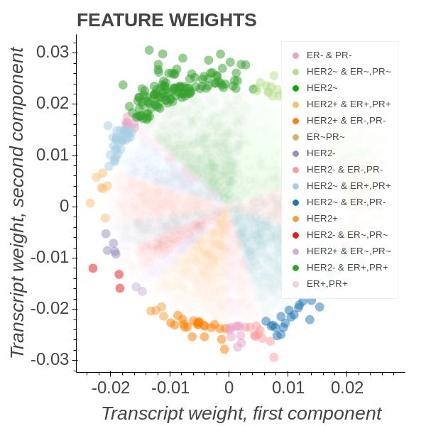
decompose and align the feature space while communicating the effect of the decompo-
sition on sample space is a well-known property of OPLS models. The OPLS methods
have long been employed for characterisation of data features, but the interpretation
often stops once the sample and feature groupings have been identified.
     Both Principle Component Analysis (PCA) [5] and OPLS create new predictor
variables often termed components. The components created by PCA maximize the
variance in each without regard for the response. In PCA, we get a large number of
components that aim to describe orthogonal variance. This affine transform can be
further exploited to evaluate the statistical significance of weight relations. Similar
to PCA, the OPLS decomposes an input matrix into unique and complementary ma-
trices. However, unlike PCA, which ultimately relies on factorising a sample centred
expression matrix along the components of maximal orthogonal variance, the OPLS
method instead decomposes an input matrix by maximizing the mutual covariance
between the feature space projection against the sample space response projection on
the OPLS predictor plane.
     The subspace plane could be any dimensionality but is most often two dimensional
such as in OPLS regression [6]. Because the weights are commonly computed via an
iterative procedure it does not necessarily converge to a good solution, it however often
does. Once the solution has been obtained then the variance in the dataset is often
better described by fewer components than in PCA. It is not strange because the goal
is to model the response by directly decomposing variance onto components describ-
ing the response. For this reason, a OPLS algorithm is similar to a two-way linear
regression ANalysis Of VAriance (ANOVA) [7]. In both methods a two-dimensional
tensor is constructed to describe the response and as such both methods are prone to
similar issues and produce similar statistical insights. We will see that, as opposed
to a two-way ANOVA model, the OPLS model also divulge information about the
directionality of the variation along an axis.
     In [8] the authors make a point that OPLS regression coefficients used in ranked
analysis do not take advantage of the multivariate nature of OPLS. This holds even
for our work, we project the decomposition down onto a univariate vector to increase
the robustness of our model interpretations.
     We define a pathway as a knowledge-based group descriptor of the transcripts. It
should not be confused with the path diagram of the latent variables [2]. Connect-
ing the weights with axis p-values and calculating pathway enrichment becomes an
important sanity check for this method. There are several knowledge-based pathway
databases [9, 10, 11, 12]. These are curated with regards to known activity of tran-
scripts and as such are not deduced from knowledge inherent in the data. In theory
a new and properly well carried out experiment should be unknown to the knowledge
database curator facilitating the group definitions. As such, if the alignment of weights
to a descriptor axis is sensible then, the pathway enrichments should convey sensible
enrichment for the groups that are under study.
     For our purposes; Given the feature and sample space description matrices (X, Y)
are described by their corresponding weights (w, c) and scores (t = Xw, u = Yc). If
the OPLS algorithm has converged on a solution, by maximizing covariance between
t and u, then w and c will be aligned on the projected subspace.
     In this work we propose a method to detect plausible research targets by an ex-
ploration of the sample space in high entropy domains through comparative plotting
of cosine alignment on OPLS [13] decomposition. Further, we demonstrate that the
OPLS decomposition can be directly utilized for: (i) p-value calculations, (ii) path-
way enrichment assessment, (iii) determining the suppression, or excitation state, of

                                           2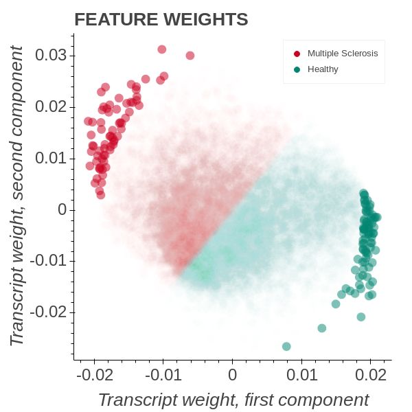
a pathway. We also demonstrate that weights associated with a simple binary one-
hot encoded, multivariate axis are equivalent to calculating traditional fold changes
between those groups.
    The remainder of the paper is structured as follows. Section 2 motivates and
describes the statistical viewpoint and exemplifies analysis usage. A number of illus-
trating analysis examples related to the previously described method process are then
presented in Section 3 in order to exemplify and validate the proposed solution. For
validation purposes a comparison to t-testing is performed. Finally, Sections 4 and 5
provide an assessment analysis and conclude from the undertaken experiments.

2     Method
For our adaptation of the OPLS method, we employ the same nomenclature as in
the work by [6]. Given the subspace vectors w ∧ t we assume that any symmetry
operations on w will commute to t. Habitually for our numerical experiments, we treat
a set of gene expressions as the feature matrix X and the patient journal, with coarse-
grained end states, as the sample response matrix Y. As such X either represent
a microarray- or a Fragments Per Kilobase of transcript per Million mapped reads
(FPKM) Ribonucleic Acid (RNA)-sequence matrix.
    The formulation of groups is done by retrieving journal value entries for a group
present in the statistical formula enclosed with parentheses and a leading ‘C’. Example

                                 Transcript ∼ C(Group)

would retrieve the Group journal value entries.
    Since OPLS maximizes the pairwise covariance score, feature weights and sample
weights are “co-linearized” in a similar way. This lets us ascribe features to sample
weights, one way is to employ tessellation. Each transcript is simply associated with
the closest sample axis. This can be either absolute coordinate proximity on the
weight projection plane or the angular proximity between the transcript and sample
axis weight. The formula for calculating the angular distance is given by the cosine
similarity:

                                                      a·b
                            d = 1 − cos(α) = 1 −
                                                   ||a|| · ||b||
   Here a, a vector, designates a transcript weight position and b a sample score
weight position, also a vector. The angle α is the angle between a and b. In summary,
we perform the steps:
    1. Use a statistical test formula that defines the group variations to test.
    2. Device an encoding data frame from journal group descriptor instances.
    3. Utilize PLS2 to find the solution to the formula using the expression matrix and
       patient (sample response) journal.
    4. Categorical membership is determined through either tessellation (euclidean dis-
       tance) or angle, cosine distance to a centroid.
    5. Calculate characteristic length scales of the prediction plane by finding the max-
       imum weights.
    6. Calculate the projected density of the weights onto the group axes defined by
       the statistical test formula.

                                            3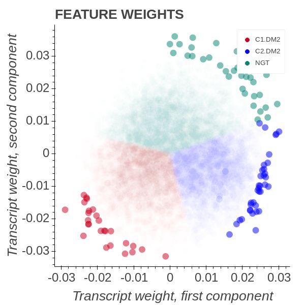
7. Calculate p-values for the projections by assuming that the weights are dis-
       tributed normally.
    8. Calculate the ranking of the weights on the projected axis, mapped in ascending
       order from zero to one.
    This can be relied upon to visualize how features associate with samples.
    Since ReactomePA [11] knowledge base is hierarchical, we also employed a hierar-
chical correction scheme similar to the elim algorithm as suggested by [14].

2.1     Implementation
We have chosen to employ the OPLS2 algorithm as implemented in the publicly avail-
able python [15] package and it also exists as an R [16, 17] package.
    All categoricals present in the patient journal are translated into a one-hot encoding
matrix. Thus all and any unique descriptors included in the group under study gets
translated into a unique axis. All formula entries that are not categoricals are treated
as real variables. The exact routine execution, visualization and calibration is covered
in the experiment code [18].
    The quantitative analysis relies on projecting the feature weight distribution onto
an axis and studying the point density distribution on that axis. The p values are
calculated from the cumulative error function for the density along the projection
axis, see supplementary code [19]. The two-way ANOVA comparison is performed
using the statsmodels [20] SciPy package.

3      Results
According to the method described in Section 2 we conducted three experiments:
     • Multiple Sclerosis (MS) microarray dataset analysis, testing sample variation to
       group interaction. Also presenting the alignment properties of angular OPLS
       model interpretation.
     • The Cancer Genome Atlas (TCGA)-BReast CAncer Gene (BRCA) two-way
       ANOVA, deducing the interaction model from the OPLS plot. Also comparing
       the analytical strength to type-2 ANOVA.
     • Diabetes MICROARRAY dataset compounded analysis with clustering enrich-
       ment for genomic impact in Type 2 Diabetes (T2D).
    The datasets for the analysis, as well as the group definition files, can all be found
online [19]. Details of the processing of the MS, as well as TCGA dataset, is also
deposited online [21].

3.1     Multiple Sclerosis and the alignment properties of OPLS
        models
The Multiple Sclerosis microarray data was obtained via the Gene Expression Omnibus
(GEO) accession number for the microarray dataset GSE219421 . 15 ‘Healthy’ controls
and 14 ‘MS’ patients were processed and used in the analysis [22]. The OPLS model
is conducting the test whether a transcript sample variation is well described by the
    1 http://www.ncbi.nlm.nih.gov/geo/

                                            4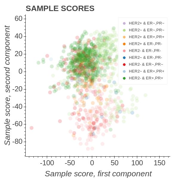
(a) The OPLS transcript weight plane        (b) The OPLS sample scores with sam-
   with weights coloured by alignment to       ples coloured by MS state
   MS state

                     Figure 1: OPLS model of the MS state.

between-group variation. We choose to express this as a statistical formula on the
form
                            Transcript ∼ C(Status)
Here the Status label can take on the values Healthy or MS.
     In Figure 1a we can see how the transcripts become aligned to the disease state.
A large number of transcripts are positioned close to origo and those that are farther
away than 99% of all transcripts are highlighted with a higher opacity. From Figure 1b,
it is clear that the OPLS model separates the cohort well. By comparing the left
and right graph we see that the transcript weights are aligned so that we only have
significant weights in the same quadrants as samples. The Y matrix, describing the
MS and Healthy subjects sample score weights are also in the same quadrants. We can
calculate the angular proximity between the sample score weights and the transcripts
feature weights and assign what transcripts are closest to a particular score weight.
This allows us to colour the transcripts according to the descriptor that best captures
their variation in the data. We can also define new vectors corresponding to different
directions on the transcript weight plane.
     In Figure 2a, we depict the negative logarithm of the OPLS p-values on the y-
axis and fold change values on the x-axis. In this case, the OPLS model describes
the separation between Healthy and MS patients and the p values are thus analogue
to t-test comparison based p values resulting in a volcano plot appearance. The axis
describing the Healthy-Multiple Sclerosis state variation p values can then be employed
to calculate pathway enrichments. In Figure 2b, the pathway enrichment has been
calculated using a Fisher exact test together with the Reactome pathway database.
For each pathway, significant genes are deduced based on a p-value cutoff equal to
0.05 and a contingency table is produced. The resulting contingency table is then
evaluated using a two-sided Fisher exact test. We choose a two-sided test because we

                                           5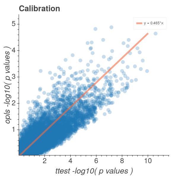
(a) The gene transcripts associated        (b) Hierarchically corrected pathway
   OPLS p values against log2 fold            enrichment.
   changes.

Figure 2: Sizes corresponds to gene ratios and the significance levels depicted
are raw p values.

employ a variational model. As such the enrichment does not correspond to an up
or down-regulated accumulation in the group but rather correspond to if the group is
important in describing the OPLS axis.
    In Figure 3 we study the gene associations calculated directly from the OPLS
feature weights. The feature associations can be calculated from the angle between
two transcripts, β, on the transcript OPLS weight plane. All pairs of cos(β) make up
an association map for the OPLS model. The values range from +1, for fully aligned,
through 0, for orthogonal, to −1 for antialigned. The OPLS solution constructs a
model surface that maximizes the variance between the Y axes. This is the reason
why the association map represents an over accentuated correlation map of the genes
depicted.
    By selecting a smaller subset of transcripts, here with q < 0.16 values, and calcu-
lating the association map we see that the significant transcripts are roughly divided
into two anti-associated clusters. Under the assumption that our coding genes produce
proteins, we may utilize string-db [9] to analyse them. We find that they enrich for
immune system activity in the specific and tertiary granule lumens. The largest clus-
ter enriches for antifungal humoral response and innate immune response in mucosa
while the second cluster enriches for publications on long non-coding RNA activity.
In the second cluster, the gene with the highest intersection among such publications
is the PSMD5 transcript. The protein of this gene has also been reported for proteomic
quantification of differentially expressed genes between MS and Healthy patients [23].
    From Figure 4a it is clear that our OPLS model derived p-values are conservative
estimates when compared to those stemming from a t-test. From Figure 4b it is

                                          6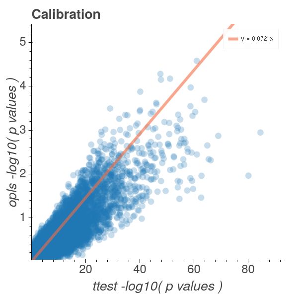
(a) The gene transcripts association (b) Quantification of the transcripts
map. Colors correspond to the co- with most significant group differences.
sine of the angle between the feature
weights.
Figure 3: Gene transcription association exploration.
(a) Volcano plot with ttest p-values (b) Comparison of the our model p-
plotted against log2 fold changes. values and traditional t-test derived p-
values.
Figure 4: MS Comparison of opls and t-test produced p-values.
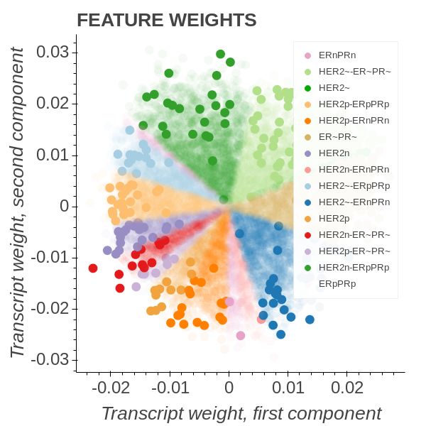
7(a) Transcript weight colored by their (b) The sample scores show that triple
hormone alignment owners. negative patients are diametrically op-
posed to HER2- & PR+, ER+ patients.
Figure 5: OPLS model of the TCGA breast cancer data set.
clear that the p-value distribution is heteroscedastic around the y ≈ 0.5x line in the
logarithmic p-value space numerically proving that we are quantifying the same type
of discoveries as the t-test, but with much more conservative estimates of the p-values.
3.2 TCGA-BRCA and the comparison with a two-way
ANOVA
In this section we study the TCGA Breast cancer dataset [24] under OPLS and a type-
2 ANOVA. Clinical parameters [25], as well as messenger Ribonucleic Acid (mRNA)
expression data from human female patients. Theses were obtained from the TCGA
website [24]. All of the downloaded samples originated from Illumina RNA-Seq data
using the High Throughput Sequencing (HTS) 3 FPKM workflow [26]. In the case
where more than one expression profile belonged to one sample id we randomly selected
one of the profiles. Sample receptor statuses [27] were stored as ER+, ER-, PR+, PR-,
HER2+, HER2- or ND in a sample journal file. This resulted in 1184 breast cancer
samples [21].
In Figure 5 we employed an OPLS model of the form
Transcript ∼ C(HER2) : C(ERPR) + C(HER2) + C(ERPR)
and coloured all the group instances with unique colours. The HER2 group describes
the HER2 receptor state while the Estrogen Receptor Progresterone Receptor (ERPR)
group describes whether or not the ER and PR receptors are in a particular state. Thus
triple-negative patients will belong to the HER2- & PR-, ER- intergenetion and triple
positive to the HER2+ & PR+, ER+. It is well known that triple-negative patients have
a poor survival outcome for breast cancer and are interesting to study in this context.
8(a) Association map of transcripts de- (b) Box plots of most significant tran-
scribing the variation along the triple scripts HER2-, PR+, ER+ patients exhibit
negative axis starkest differences towards triple neg-
atives
Figure 6: OPLS model association map of the TCGA breast cancer data set.
Figure 5b shows that triple-negative patients amass in the most southern parts of the
lower quadrants. Diametrically opposed we find the patients bearing the interaction
combination belonging to HER2- & PR+, ER+. We note that the triple-positive group
form an angle of roughly 110 degrees to the triple-negative group. From here on the
call the triple-negative towards HER2-, PR+, ER+ axis the high-risk axis.
Among the genes with the strongest association to the high-risk axis, we find ESR1,
CXXC5, GREB1, FOXA1 and GATA3. They enrich [9] for estrogen-dependent gene expres-
sion in Reactome as well as the prostate gland and uterus development in biological
processes [12]. We only have women in the data so we safely assume that the prostate
gland enrichment is due to the interaction of these genes with the progesterone receptor
in men.
In Figure 6b, we find the traditional quantification of the transcript data. Triple-
negative patients are remarkably different from the other groups. We also show both
triple-positive as well as HER2-, PR+ and ER+ patient groupings. The OPLS model
in Figure 5b conveyed the information that HER2-, PR+, ER+ combination are anti
associated to the triple negatives and we can also see that the biggest difference in
the boxplots of Figure 6b is found between the triple-negative and HER2-, PR+, ER+
group. It is also becomes apparent that the gene cluster associated with being up
in triple-negative patients belong to PSAT1, TTL4, FOXC1, USB1, PDSS1, YBX1, KCMF1,
YBX1P10 and DSC2. It constitutes a novel cluster for describing triple-negative patients
and it is only when evaluated along the high-risk axis that the full picture emerges.
These results would not be complete without mentioning the statistical properties
of the weights. Since there is no warranty that OPLS models converge on any specific
9(a) The p values produced by the OPLS (b) OPLS model with all transcripts having
0.05
model as well as the intermittent o and final two-way ANOVA q < 10455 shown with full
q values. opacity.
residual distribution this can become convoluted. The maximisation of variance on
the common subspace plane implies that a solution would minimize the OPLS models
squared residual. In using our formalism we can study the same formula using both an
ANOVA as well as an OPLS model. In Figure 7b we show the same statistical model,
Transcript ∼ C(HER2) : C(ERPR) + C(HER2) + C(ERPR)
produces qualitatively similar results.
In Figure 7a depicts the OPLS model where all the interaction categories of
Transcript ∼ C(HER2) : C(ERPR)
are shown. The transcripts are also modelled using a two-way ANOVA and all tran-
0.05
scripts having an interaction with a q < 10455 are depicted in full opacity. Two
realizations are immediate. The first is that the ANOVA results are qualitatively sim-
ilar to those of the OPLS, with a large density of significant ANOVA transcripts being
found on the rim of the OPLS weight plane. Our OPLS model, however, offers an im-
provement in that we may determine not just the specific interaction pair associated
with which transcript but also the direction. From our model, we can recognize that
TTLL4 will be scaling in magnitude with the triple-negative state as well as being sig-
nificantly different from the other groupings. The traditional box plot quantification
in Figure 6b is important but not essential. We further explore our OPLS p-values
and it is clear from Figure 7a that we have a large accumulation of weights near the
centre. This also means that we are more prone to false discoveries near the centre.
One can directly correct for this in the q value calculation by assuming that the False
Discovery Rate (FDR) scale linearly with the Fractional Rank (FR) of the list of p
values, which is quantified by:
ranks(p)
fr(p) =
length(p)
10(a) Volcano plot with ttest p-values (b) Comparison of the our model p-
plotted against log2 fold changes. values and traditional t-test derived p-
values.
Figure 8: TCGA Comparison of OPLS and t-test produced p-values.
Instead of assuming a constant FDR [28] across p values, often set equal to 1, for the
q value calculation we set it to scale using the FR formula. These scaled p values
are here dubbed o values and are only used to show the effect of this scaling. The
final q values are showed in Figure 7b. We recognize that the OPLS transcripts with
significant interaction all belong to the rim of the categories defined by the axis studied
(here the far edge of the HER2+, PR-, ER- axis).
By inspecting Figure 8 we can see that the axis found also generates the high
significance interaction using a t-test. One could numerically perfom all pairwise t-
tests, we will refrain from doing, in order to draw a conclusion about wether this
axis has the highest t-test significance. Instead we note that, from Figure 5a, the
axis grouping containing the triple negative samples as well as their diametrically
opposed group is the HER2-&ER-,PR- HER2-&ER+,PR+ pair and not the triple positive
group. The t-test significance magnitude drops to half of that obtained from the axis
reported as the most important axis when changed to triple negatives paired against
triple positives. From Figure 8b the method remains heteroscedastic around a power
law relation. However here our p-values roughly fall on the y ≈ x ∗ 0.072 line in log
space. As such we remain conservative in our p-value quantification with respect to a
t-test along a comparable axis. In this case our p-values are still of the same order of
magnitude as in Figure 4a. This is due to the fact that they are computed from the
transcript position and the transcript density. Since this is decoupled from the samples
in the OPLS model we can evaluate it across an arbitrary sample axis. The transcript
density is defined by roughly the same amount of transcripts in the Multiple Sclerosis
and Breast Cancer cases and the transcript p-value magnitudes is therefore comparable
and of the same order of magnitude for both of the OPLS models. The OPLS weight
alignment become more reliable as more samples are added but this information is
not directly conveyed to the OPLS p-values. We note that, as in Figure 4b, that our
11Figure 9: T2D & NGT OPLS model with all transcripts.
p-values are conservative. By noting that we are projecting onto a spherical solution
space (2-dimensional) where the opls axis (1-dimensional) is set by the sample space
we realize that our axis p-values will calibrate towards t-test derived p-values, across
the same sample grouping axis as in equation 1
r
Nsamples
2π
popls,axis ≈ pt−test,axis (1)
The main advantage of our method is that we can, using an unbiased method,
identify the group that is diametrically opposed to the disease group.
3.3 Diabetes Microarray Analysis
Type 2 Diabetes is a metabolic disease on the rise in the general populous. It is fur-
thermore influenced by both lifestyle choices as well as genetic factors. Understanding
the detailed balance required for this disease phenotype to emerge is important to
achieve better therapies and quality of life of those affected by it. The understanding
of altered metabolism is also of great importance since many diseases are associated
with altered cell and tissue metabolism [29].
There is an increasing amount of evidence that type 2 diabetes T2D, or Diabetes
Mellitus 2 (DM2), disease phenotype constitutes several underlying metabolic disease
phenotypes [30].
Here we have chosen to study human DM2 data from the Broad Institute [29].
Suspecting that we have more than a single type of DM2 patients we first segmented the
data. This was done by employing approximative density clustering as implemented
in our package [19]. Because of the limited number of samples (18) we stopped once
we had obtained the two most separated sample groups. We thereby obtain two well-
separated DM2 cluster types that we name C1.DM2 and C2.DM2 where the cluster index
is the inverted cluster size rank.
12(a) All the edge weight associations be- (b) The association map of the largest
low q < 0.005 DM2 group and NGT variation, q <
0.0001
Figure 10: Complete OPLS association maps.
In Figure 9 we see that the second cluster consists of only three samples. They form
a group well-separated from the rest but lying close to orthogonal to the NGT group.
The first cluster forms an axis with the NGT group with weights being positioned
opposed to one another. Using our OPLS model we would believe that they constitute
a smaller DM2 phenotype subset with distinct metabolic alterations. By studying the
p-values associations on the rim of the entire OPLS graph we find that FAM35A have
0.05
q < Ntranscripts and aligning with the C1.DM2 axis. FAM35A is known to be a favourable
prognostic marker of glioma and colo-rectal cancer [31]. By allowing ourself to study
genes with q < 0.005 we obtain the association map in Figure 10a.
In Figure 10 we can clearly discern four transcript clusters. The first two corre-
spond to transcripts that are positively associating with being healthy. Those tran-
scripts enrich for Cyclin C activity, which is known for controlling nuclear cell divi-
sion [32]. The third cluster is positioned near the centre of the association map on the
left and is close to orthogonal to the other clusters.
This cluster consists of transcripts that enrich [9] for striated muscle contrac-
tion [11] and organ morphogenesis [12]. Most of the enrichment signal is, however,
coming from the MYL2, ACTA1, CLDN1, POU4F1, CRX and TNF group. This third clus-
ter belongs to the C2.DM2 group indicating that these three individuals, albeit being
diabetic, might have dramatically different muscle metabolism.
The first and biggest cluster belong is the C1.DM2 samples visible in Figure 10. Four
transcripts reach high significance and together enrich for ATP binding activity. The
9 high significance transcripts aligning with this axis enrich [9] for DeoxyriboNucleic
Acid (DNA) repair and DNA metabolism. Taken together with the full C1.DM2-NGT
axis transcripts enrich for activity in the condensed nuclear chromosome. By allowing
ourselves to be less strict and studying enrichments at lower confidence corresponding
to the C1.DM2-NGT transcripts in Figure 10a.
13Figure 11: T2D & NGT PCA model with all transcripts.
Approximate density clustering is similar to agglomerative hierarchical clustering
but instead of building a distance hierarchy we try to find the best sample grouping
describing the sample space.
All other things being equal we can compare Figure 9 and Figure 11 and see that
OPLS, by its very nature, better separates the data. In Figure 11 we see that the
three samples who have their own cluster in Figure 9 also correspond to outliers when
employing PCA.
4 Discussion
The discussion is divided into three subsections corresponding to the previously pre-
sented use cases in the result section.
4.1 Multiple Sclerosis
Regarding the multiple sclerosis use case we see from Figure 2 in Section 3.1 that
the major pathways deduced are complex I biogenesis and neutrophil granulation,
pathways which are affiliated with increased metabolism and immune system activity.
Compartment enrichment analysis, also utilizing a two-sided Fisher exact test, of our
p-values tells us that the dataset is mainly active in the cytosol, nucleoplasm and
ficolin-1-rich granule membrane. This conveys the picture that we are dealing with
neutrophil degranulation and metabolism of surface membranes. This is aligned with
the common view that MS is associated with demyelination of axon myelin. Roughly
translating into altered lipid metabolism by the immune system.
Our modelling scheme shows weaker statistical power than other methods but
recovers fundamental and broad descriptive knowledge about the dataset. We also
identify a small subset of significant genes that are differentially expressed in the cohort
and share an intersection with proteomic analysis. Both the proteomic derived set as
14well as our OPLS transcriptome analysis does not share a common intersection with the
Genome Wide Association Study (GWAS) published together with the dataset that
we employed. This analysis method should as such be viewed as a complementary
method for producing a data-driven story of the cohort as well as targets of interest
for use in further biological validation. In this section, we have shown how the Y
matrix alignments translate into the feature space of OPLS models.
Looking at Figure 3a and allowing ourself down into the first 100 significant OPLS
genes, with a p < 0.0002 value, we see a common intersection set between our results
and the [23] proteins. These are TES, CLTC, SIN3A as well as PSMD5 and known to
influence RUNX1 transcription pathways.
4.2 Breast Cancer
In the breast cancer use case; the Forkhead box (FOX) C1 transcript is thought to be
a possible target in nasopharyngeal carcinoma [33]. FOXA1 is similarly known to be
correlated with GATA3, Progesteron receptor protein expression and clinical outcomes
in breast cancer [27] as well as prostate cancer [34]. However, some of the associations
in Figure 6a are new and might be interesting targets for further biological validation.
It is worth further emphasis that these gene transcripts correspond to the outliers
lying on the axis connecting the triple-negative and the HER2-, PR+, ER+ in the OPLS
feature weight plane.
4.3 Type 2 Diabetes
Hierarchical modelling or agglomerative hierarchical clustering are well-known meth-
ods of partitioning one’s data. Traditionally, building hierarchical models are done
via curating knowledge and manually constructing a hierarchy [11, 30]. One can also
choose to computationally construct hierarchical data structures using agglomerative
hierarchical clustering [35] or simply try to find the grouping that will separate the
density the most [19].
Guided by Figure 10 we see an enrichment [9] for Guanosine TriPhosphate (GTP)
metabolism in the mitochondria. We know that mitochondrial GTP metabolism is
essential for glucose-dependent insulin secretion [36]. It is known that this will lead to
disrupted oxidative phosphorylation and an altered mitochondrial membrane poten-
tial [35]. Furthermore, mitochondria maintain oxidative phosphorylation by creating a
membrane potential, also implying an altered membrane potential will lead to altered
oxidative phosphorylation [37]. This together is indicative that Adenosine TriPhos-
phate (ATP) synthesis might be inhibited, for the diabetics, in the mitochondria [38].
These findings are qualitatively similar to those reported by [29]. This is indeed good
news since we are studying people whom, by definition, have inhibited metabolic reg-
ulatory control of glucose and insulin.
5 Conclusions
In this work we have developed a new analysis method and code library, as described
in Section 2 and 2.1, for use in bioinformatic analysis. We have demonstrated the use
of OPLS models for transcriptomic analysis on three different mRNA data sets, MS
(Section 3.1), TCGA-BRCA (Section 3.2) and T2D (Section 3.3). Our models produce
unbiased sensible descriptions of the endpoint endogen states where we can relate what
15we see in the data to known properties of the human patient samples that we studied,
as discussed in Section 4. We have shown how the alignment of the sample to feature
scores translate into the ability to interpret feature weights in the context of the sample
weights. As such the realization that the weights of the feature and sample descriptor
matrices are aligned facilitates the use of the feature weights directly in traditional
pathway analysis methods. This also means that a high weight in the direction of a
predictor axis will equate to large, between-group, difference quantifications lying on
that axis.
From this, several new and sensible interpretations of the data emerge. We can
also confirm previously known properties of the samples. We find a gene cluster which
follows the triple-negative breast cancer patients which have interesting suggestion
targets for continued validation.
OPLS models are employed in such diverse research fields as financial forecast-
ing [39], brain imaging [40] as well as environmental spatial characterization and fore-
casting [41]. We believe as such that the method is suitable as decision support for
providing global suggestions of future study in high entropy domains. To our knowl-
edge, looking at other OPLS model applications, no one explores the orientation, or
vector alignment, properties of such models.
16References
[1] Wold S, Albano C, Dunn WJ, Edlund U, Esbensen K, Geladi P, Hellberg S,
Johansson E, Lindberg W, Sjöström M. 1984 Multivariate Data Analysis in
Chemistry. In Kowalski BR, editor, Chemometrics: Mathematics and Statistics
in Chemistry , pp. 17–95. Dordrecht: Springer Netherlands.
[2] Wegelin JA. 2000 A Survey of Partial Least Squares (PLS) Methods, with Em-
phasis on the Two-Block Case. .
[3] Rothenberg DO, Yang H, Chen M, Zhang W, Zhang L. 2019 Metabolome and
Transcriptome Sequencing Analysis Reveals Anthocyanin Metabolism in Pink
Flowers of Anthocyanin-Rich Tea (Camellia Sinensis). Molecules 24.
[4] Eriksson L, Byrne T, Johansson E, Trygg J, Vikström C. 2013 Multi- and
Megavariate Data Analysis Basic Principles and Applications, Third Revised Edi-
tion. Umetrics Academy.
[5] Abdi H, Williams LJ. 2010 Principal Component Analysis: Principal Component
Analysis. Wiley Interdisciplinary Reviews: Computational Statistics 2, 433–459.
[6] Rosipal R, Krämer N. 2006 Overview and Recent Advances in Partial Least
Squares. In Saunders C, Grobelnik M, Gunn S, Shawe-Taylor J, editors, Subspace,
Latent Structure and Feature Selection pp. 34–51 Berlin, Heidelberg. Springer
Berlin Heidelberg.
[7] Fisher RA. 1919 XV.—The Correlation between Relatives on the Supposition
of Mendelian Inheritance.. Transactions of the Royal Society of Edinburgh 52,
399–433.
[8] Tapp HS, Kemsley EK. 2009 Notes on the Practical Utility of OPLS. TrAC Trends
in Analytical Chemistry 28, 1322–1327.
[9] Szklarczyk D, Gable AL, Lyon D, Junge A, Wyder S, Huerta-Cepas J, Simonovic
M, Doncheva NT, Morris JH, Bork P, Jensen LJ, von Mering C. 2019 STRING
V11: Protein-Protein Association Networks with Increased Coverage, Support-
ing Functional Discovery in Genome-Wide Experimental Datasets.. Nucleic acids
research 47, D607–D613.
[10] Kanehisa M, Goto S. 2000 KEGG: Kyoto Encyclopedia of Genes and Genomes.
Nucleic Acids Research 28, 27–30.
[11] Jassal B, Matthews L, Viteri G, Gong C, Lorente P, Fabregat A, Sidiropoulos
K, Cook J, Gillespie M, Haw R, Loney F, May B, Milacic M, Rothfels K, Sevilla
C, Shamovsky V, Shorser S, Varusai T, Weiser J, Wu G, Stein L, Hermjakob
H, D’Eustachio P. 2019 The Reactome Pathway Knowledgebase. Nucleic Acids
Research.
[12] Mi H, Muruganujan A, Ebert D, Huang X, Thomas PD. 2018 PANTHER Version
14: More Genomes, a New PANTHER GO-Slim and Improvements in Enrichment
Analysis Tools. Nucleic Acids Research 47, D419–D426.
[13] Trygg J, Wold S. 2002 Orthogonal Projections to Latent Structures (O-PLS).
Journal of Chemometrics 16, 119–128.
[14] Alexa A, Rahnenfuhrer J, Lengauer T. 2006 Improved Scoring of Functional
Groups from Gene Expression Data by Decorrelating GO Graph Structure. Bioin-
formatics 22, 1600–1607.
17[15] Pedregosa F, Varoquaux G, Gramfort A, Michel V, Thirion B, Grisel O, Blondel
M, Prettenhofer P, Weiss R, Dubourg V, Vanderplas J, Passos A, Cournapeau
D, Brucher M, Perrot M, Duchesnay E. 2011 Scikit-Learn: Machine Learning in
Python. Journal of Machine Learning Research 12, 2825–2830.
[16] Geladi P, Kowalski BR. 1986 Partial Least-Squares Regression: A Tutorial. An-
alytica Chimica Acta 185, 1–17.
[17] Höskuldsson A. 1988 PLS Regression Methods. Journal of Chemometrics 2, 211–
228.
[18] Tjörnhammar E, Tjörnhammar R. 2020 Exploratory Projection to Latent Struc-
ture Models for Use in Transcriptomic Analysis, Experiment Code. .
[19] Tjörnhammar R. 2019 Impetuous-Gfa. .
[20] Seabold S, Perktold J. 2010 Statsmodels: Econometric and Statistical Modeling
with Python. In 9th Python in Science Conference.
[21] Tjörnhammar R. 2019 MS and TCGA Dataset. .
[22] Kemppinen AK, Kaprio J, Palotie A, Saarela J. 2011 Systematic Review of
Genome-Wide Expression Studies in Multiple Sclerosis. BMJ Open 1.
[23] Berge T, Eriksson A, Brorson IS, Høgestøl EA, Berg-Hansen P, Døskeland A,
Mjaavatten O, Bos SD, Harbo HF, Berven F. 2019 Quantitative Proteomic Anal-
yses of CD4(+) and CD8(+) T Cells Reveal Differentially Expressed Proteins in
Multiple Sclerosis Patients and Healthy Controls. Clinical proteomics 16, 19–19.
[24] Koboldt DC, Fulton RS, McLellan MD, Schmidt H, Kalicki-Veizer J, McMichael
JF, Fulton LL, Dooling DJ, Ding L, Mardis ER, Wilson RK, Ally A, Balasun-
daram M, Butterfield YSN, Carlsen R, Carter C, Chu A, Chuah E, Chun HJE,
Coope RJN, Dhalla N, Guin R, Hirst C, Hirst M, Holt RA, Lee D, Li HI, Mayo
M, Moore RA, Mungall AJ, Pleasance E, Gordon Robertson A, Schein JE, Shafiei
A, Sipahimalani P, Slobodan JR, Stoll D, Tam A, Thiessen N, Varhol RJ, Wye
N, Zeng T, Zhao Y, Birol I, Jones SJM, Marra MA, Cherniack AD, Saksena G,
Onofrio RC, Pho NH, Carter SL, Schumacher SE, Tabak B, Hernandez B, Gentry
J, Nguyen H, Crenshaw A, Ardlie K, Beroukhim R, Winckler W, Getz G, Gabriel
SB, Meyerson M, Chin L, Park PJ, Kucherlapati R, Hoadley KA, Todd Auman
J, Fan C, Turman YJ, Shi Y, Li L, Topal MD, He X, Chao HH, Prat A, Silva
GO, Iglesia MD, Zhao W, Usary J, Berg JS, Adams M, Booker J, Wu J, Gula-
bani A, Bodenheimer T, Hoyle AP, Simons JV, Soloway MG, Mose LE, Jefferys
SR, Balu S, Parker JS, Neil Hayes D, Perou CM, Malik S, Mahurkar S, Shen H,
Weisenberger DJ, Triche Jr T, Lai PH, Bootwalla MS, Maglinte DT, Berman BP,
Van Den Berg DJ, Baylin SB, Laird PW, Creighton CJ, Donehower LA, Getz
G, Noble M, Voet D, Saksena G, Gehlenborg N, DiCara D, Zhang J, Zhang H,
Wu CJ, Yingchun Liu S, Lawrence MS, Zou L, Sivachenko A, Lin P, Stojanov
P, Jing R, Cho J, Sinha R, Park RW, Nazaire MD, Robinson J, Thorvaldsdottir
H, Mesirov J, Park PJ, Chin L, Reynolds S, Kreisberg RB, Bernard B, Bressler
R, Erkkila T, Lin J, Thorsson V, Zhang W, Shmulevich I, Ciriello G, Weinhold
N, Schultz N, Gao J, Cerami E, Gross B, Jacobsen A, Sinha R, Arman Aksoy
B, Antipin Y, Reva B, Shen R, Taylor BS, Ladanyi M, Sander C, Anur P, Spell-
man PT, Lu Y, Liu W, Verhaak RRG, Mills GB, Akbani R, Zhang N, Broom
BM, Casasent TD, Wakefield C, Unruh AK, Baggerly K, Coombes K, Weinstein
JN, Haussler D, Benz CC, Stuart JM, Benz SC, Zhu J, Szeto CC, Scott GK,
Yau C, Paull EO, Carlin D, Wong C, Sokolov A, Thusberg J, Mooney S, Ng S,
18Goldstein TC, Ellrott K, Grifford M, Wilks C, Ma S, Craft B, Yan C, Hu Y,
Meerzaman D, Gastier-Foster JM, Bowen J, Ramirez NC, Black AD, Pyatt RE,
White P, Zmuda EJ, Frick J, Lichtenberg TM, Brookens R, George MM, Gerken
MA, Harper HA, Leraas KM, Wise LJ, Tabler TR, McAllister C, Barr T, Hart-
Kothari M, Tarvin K, Saller C, Sandusky G, Mitchell C, Iacocca MV, Brown J,
Rabeno B, Czerwinski C, Petrelli N, Dolzhansky O, Abramov M, Voronina O,
Potapova O, Marks JR, Suchorska WM, Murawa D, Kycler W, Ibbs M, Korski
K, Spychała A, Murawa P, Brzeziński JJ, Perz H, Łaźniak R, Teresiak M, Tatka
H, Leporowska E, Bogusz-Czerniewicz M, Malicki J, Mackiewicz A, Wiznerowicz
M, Van Le X, Kohl B, Viet Tien N, Thorp R, Van Bang N, Sussman H, Duc Phu
B, Hajek R, Phi Hung N, Viet The Phuong T, Quyet Thang H, Zaki Khan K,
Penny R, Mallery D, Curley E, Shelton C, Yena P, Ingle JN, Couch FJ, Lingle
WL, King TA, Maria Gonzalez-Angulo A, Mills GB, Dyer MD, Liu S, Meng X,
Patangan M, The Cancer Genome Atlas Network, Genome sequencing centres:
Washington University in St Louis, Genome characterization centres: BC Can-
cer Agency, Broad Institute, Brigham & Women’s Hospital & Harvard Medical
School, University of North Carolina CH, University of Southern California/Johns
Hopkins, Genome data analysis: Baylor College of Medicine, Institute for Sys-
tems Biology, Memorial Sloan-Kettering Cancer Center, Oregon Health & Science
University, The University of Texas MD Anderson Cancer Center, University of
California SCI, NCI, Biospecimen core resource: Nationwide Children’s Hospital
Biospecimen Core Resource, Tissue source sites: ABS-IUPUI, Christiana, Cure-
line, Duke University Medical Center, The Greater Poland Cancer Centre, ILSBio,
International Genomics Consortium, Mayo Clinic, MSKCC, MD Anderson Can-
cer Center. 2012 Comprehensive Molecular Portraits of Human Breast Tumours.
Nature 490, 61–70.
[25] Tao M, Song T, Du W, Han S, Zuo C, Li Y, Wang Y, Yang Z. 2019 Classifying
Breast Cancer Subtypes Using Multiple Kernel Learning Based on Omics Data..
Genes 10.
[26] Anders S, Pyl PT, Huber W. 2015 HTSeq—a Python Framework to Work with
High-Throughput Sequencing Data. Bioinformatics 31, 166–169.
[27] Ross-Innes CS, Stark R, Teschendorff AE, Holmes KA, Ali HR, Dunning MJ,
Brown GD, Gojis O, Ellis IO, Green AR, Ali S, Chin SF, Palmieri C, Caldas
C, Carroll JS. 2012 Differential Oestrogen Receptor Binding Is Associated with
Clinical Outcome in Breast Cancer. Nature 481, 389–393.
[28] Storey JD, Tibshirani R. 2003 Statistical Significance for Genomewide Studies.
Proceedings of the National Academy of Sciences 100, 9440–9445.
[29] Mootha VK, Lindgren CM, Eriksson KF, Subramanian A, Sihag S, Lehar J,
Puigserver P, Carlsson E, Ridderstråle M, Laurila E, Houstis N, Daly MJ, Patter-
son N, Mesirov JP, Golub TR, Tamayo P, Spiegelman B, Lander ES, Hirschhorn
JN, Altshuler D, Groop LC. 2003 PGC-1α-Responsive Genes Involved in Ox-
idative Phosphorylation Are Coordinately Downregulated in Human Diabetes.
Nature Genetics 34, 267–273.
[30] Ahlqvist E, Storm P, Käräjämäki A, Martinell M, Dorkhan M, Carlsson A,
Vikman P, Prasad RB, Aly DM, Almgren P, Wessman Y, Shaat N, Spégel P,
Mulder H, Lindholm E, Melander O, Hansson O, Malmqvist U, Lernmark Å,
Lahti K, Forsén T, Tuomi T, Rosengren AH, Groop L. 2018 Novel Subgroups
of Adult-Onset Diabetes and Their Association with Outcomes: A Data-Driven
19Cluster Analysis of Six Variables. The Lancet Diabetes & Endocrinology 6, 361–
369.
[31] Uhlén M, Fagerberg L, Hallström BM, Lindskog C, Oksvold P, Mardinoglu A,
Sivertsson Å, Kampf C, Sjöstedt E, Asplund A, Olsson I, Edlund K, Lundberg E,
Navani S, Szigyarto CAK, Odeberg J, Djureinovic D, Takanen JO, Hober S, Alm
T, Edqvist PH, Berling H, Tegel H, Mulder J, Rockberg J, Nilsson P, Schwenk
JM, Hamsten M, von Feilitzen K, Forsberg M, Persson L, Johansson F, Zwahlen
M, von Heijne G, Nielsen J, Pontén F. 2015 Tissue-Based Map of the Human
Proteome. Science 347, 1260419.
[32] Galderisi U, Jori FP, Giordano A. 2003 Cell Cycle Regulation and Neural Differ-
entiation. Oncogene 22, 5208–5219.
[33] Ou-Yang L, Xiao SJ, Liu P, Yi SJ, Zhang XL, Ou-Yang S, Tan SK. 2015 Forkhead
Box C1 Induces Epithelial-mesenchymal Transition and Is a Potential Therapeutic
Target in Nasopharyngeal Carcinoma.. Molecular Medicine Reports 12, 8003–
8009.
[34] Barbieri CE, Baca SC, Lawrence MS, Demichelis F, Blattner M, Theurillat JP,
White TA, Stojanov P, Van Allen E, Stransky N, Nickerson E, Chae SS, Boysen
G, Auclair D, Onofrio RC, Park K, Kitabayashi N, MacDonald TY, Sheikh K,
Vuong T, Guiducci C, Cibulskis K, Sivachenko A, Carter SL, Saksena G, Voet
D, Hussain WM, Ramos AH, Winckler W, Redman MC, Ardlie K, Tewari AK,
Mosquera JM, Rupp N, Wild PJ, Moch H, Morrissey C, Nelson PS, Kantoff PW,
Gabriel SB, Golub TR, Meyerson M, Lander ES, Getz G, Rubin MA, Garraway
LA. 2012 Exome Sequencing Identifies Recurrent SPOP, FOXA1 and MED12
Mutations in Prostate Cancer. Nature Genetics 44, 685–689.
[35] Mehta P, Bukov M, Wang CH, Day AG, Richardson C, Fisher CK, Schwab DJ.
2019 A High-Bias, Low-Variance Introduction to Machine Learning for Physicists.
A high-bias, low-variance introduction to Machine Learning for physicists 810,
1–124.
[36] Kibbey RG, Pongratz RL, Romanelli AJ, Wollheim CB, Cline GW, Shulman GI.
2007 Mitochondrial GTP Regulates Glucose-Stimulated Insulin Secretion. Cell
Metabolism 5, 253–264.
[37] Momcilovic M, Jones A, Bailey ST, Waldmann CM, Li R, Lee JT, Abdelhady
G, Gomez A, Holloway T, Schmid E, Stout D, Fishbein MC, Stiles L, Dabir DV,
Dubinett SM, Christofk H, Shirihai O, Koehler CM, Sadeghi S, Shackelford DB.
2019 In Vivo Imaging of Mitochondrial Membrane Potential in Non-Small-Cell
Lung Cancer. Nature 575, 380–384.
[38] Sivitz WI, Yorek MA. 2010 Mitochondrial Dysfunction in Diabetes: From Molec-
ular Mechanisms to Functional Significance and Therapeutic Opportunities. An-
tioxidants & redox signaling 12, 537–577.
[39] Huang SC, Wu TK. 2010 Integrating Recurrent SOM with Wavelet-Based Kernel
Partial Least Square Regressions for Financial Forecasting. Expert Systems with
Applications 37, 5698–5705.
[40] Abdi H. 2010 Partial Least Squares Regression and Projection on Latent Struc-
ture Regression (PLS Regression): PLS REGRESSION. Wiley Interdisciplinary
Reviews: Computational Statistics 2, 97–106.
20[41] Thioulouse J, Chessel D, Champely S. 1995 Multivariate Analysis of Spatial Pat-
terns: A Unified Approach to Local and Global Structures. Environmental and
Ecological Statistics 2, 1–14.
21You can also read