From the middle stratosphere to the surface, using nitrous oxide to constrain the stratosphere-troposphere exchange of ozone
←
→
Page content transcription
If your browser does not render page correctly, please read the page content below

Research article
Atmos. Chem. Phys., 22, 2079–2093, 2022
https://doi.org/10.5194/acp-22-2079-2022
© Author(s) 2022. This work is distributed under
the Creative Commons Attribution 4.0 License.

            From the middle stratosphere to the surface, using
         nitrous oxide to constrain the stratosphere–troposphere
                            exchange of ozone
                                               Daniel J. Ruiz and Michael J. Prather
              Department of Earth System Science, University of California Irvine, Irvine, CA 92697-3100, USA
                                         Correspondence: Daniel J. Ruiz (djruiz@uci.edu)

                                       Received: 29 July 2021 – Discussion started: 6 August 2021
                         Revised: 7 December 2021 – Accepted: 7 December 2021 – Published: 15 February 2022

       Abstract. Stratosphere–troposphere exchange (STE) is an important source of tropospheric ozone, affecting
       all of atmospheric chemistry, climate, and air quality. The study of impacts needs STE fluxes to be resolved by
       latitude and month, and for this, we rely on global chemistry models, whose results diverge greatly. Overall, we
       lack guidance from model–measurement metrics that inform us about processes and patterns related to the STE
       flux of ozone (O3 ). In this work, we use modeled tracers (N2 O and CFCl3 ), whose distributions and budgets
       can be constrained by satellite and surface observations, allowing us to follow stratospheric signals across the
       tropopause. The satellite-derived photochemical loss of N2 O on annual and quasi-biennial cycles can be matched
       by the models. The STE flux of N2 O-depleted air in our chemistry transport model drives surface variability that
       closely matches observed fluctuations on both annual and quasi-biennial cycles, confirming the modeled flux.
       The observed tracer correlations between N2 O and O3 in the lowermost stratosphere provide a hemispheric
       scaling of the N2 O STE flux to that of O3 . For N2 O and CFCl3 , we model greater southern hemispheric STE
       fluxes, a result supported by some metrics, but counter to the prevailing theory of wave-driven stratospheric
       circulation. The STE flux of O3 , however, is predominantly northern hemispheric, but evidence shows that this
       is caused by the Antarctic ozone hole reducing southern hemispheric O3 STE by 14 %. Our best estimate of the
       current STE O3 flux based on a range of constraints is 400 Tg(O3 ) yr−1 , with a 1σ uncertainty of ±15 % and
       with a NH : SH ratio ranging from 50 : 50 to 60 : 40. We identify a range of observational metrics that can better
       constrain the modeled STE O3 flux in future assessments.

1   Introduction and background                                        et al., 1997; Olsen et al., 2004; Yang et al., 2016). The uncer-
                                                                       tainty in these estimates does not effectively constrain the
The influx of stratospheric ozone (O3 ) into the troposphere           wide range found in the models being used to project future
affects its distribution, variability, lifetime, and, thus, its role   ozone (Young et al., 2013, 2018; Griffiths et al., 2021). Here
in driving climate change and surface air pollution (Zeng et           we present the case for using the observed variations in ni-
al., 2010; Hess et al., 2015; Williams et al., 2019). The net          trous oxide (N2 O) from the middle stratosphere to the surface
stratosphere-to-troposphere exchange (STE) flux of O3 has a            in order to constrain the STE flux of O3 . A similar case has
regular seasonal cycle in each hemisphere that is an impor-            been made for the radionuclide 7 Be (Liu et al., 2016), but
tant part of the tropospheric O3 budget (Stohl et al., 2003).          N2 O has a wealth of model–observation metrics on hemi-
Such fluxes are not directly observable, and we rely on ob-            spheric, seasonal, and interannual scales that constrain its
servational estimates using trace gas ratios, in particular the        STE flux very well (Prather et al., 2015; Ruiz et al., 2021).
O3 : N2 O ratio in the lower stratosphere (Murphy and Fahey,              Ozone-rich stratospheric air has been photochemically
1994; McLinden et al., 2000), or dynamical calculations us-            aged and is depleted in trace gases such as N2 O and chlo-
ing measured/modeled winds and O3 abundances (Gettelman                rofluorocarbons (CFCs). For these trace gases, the overall cir-

Published by Copernicus Publications on behalf of the European Geosciences Union.
2080                                                  D. J. Ruiz and M. J. Prather: From the middle stratosphere to the surface

culation from tropospheric sources to stratospheric destruc-         Forecasts (ECMWF) Integrated Forecasting System (IFS;
tion and back is part of the lifecycle that maintains their          cycle 38r1; T159L60) for the years 1990–2017, as are the cal-
global abundance (Holton, 1990). For N2 O and CFCs, this             culations in R2021. The CTM uses the IFS native 160 × 320
cycle of (i) loss in the middle to upper stratosphere, (ii) trans-   Gauss grid (∼ 1.1◦ ) with 60 layers, about 35 of which are
port to the lowermost stratosphere (Holton et al., 1995), and        in the troposphere. The stratospheric chemistry uses the lin-
then (iii) influx into the troposphere produces surface vari-        earized ozone model Linoz v3 and includes O3 , N2 O, NOy ,
ations not related to surface emissions (Hamilton and Fan,           CH4 , and F11 as transported trace gases (Hsu and Prather,
2000; Nevison et al., 2004; Hirsch et al., 2006; Montzka et          2010; Prather et al., 2015; Ruiz et al., 2021). There is no tro-
al., 2018; Ray et al., 2020; Ruiz et al., 2021). In this work,       pospheric chemistry but rather a boundary layer e-fold to a
we relate our modeled STE fluxes to variations at the surface        specified abundance or a surface boundary reset to an abun-
and throughout the stratosphere, linking the fluxes of N2 O          dance. Equivalent effective stratospheric chlorine levels are
to O3 through stratospheric measurements. Our goal is to de-         high enough to drive an Antarctic ozone hole, which is ob-
velop a set of model metrics founded on observations that are        served throughout this period. Thus, the ozone hole chem-
related to the STE O3 flux and can be used with an ensemble          istry in Linoz v3 is activated for all years, and the amount
of models to determine a better, constrained estimate for the        of O3 depleted depends on the Antarctic meteorology of that
flux, including seasonal, interannual, and hemispheric pat-          year (Hsu and Prather, 2010).
terns. This approach is similar to efforts involving the ozone          The STE flux is calculated using the e90 definition of tro-
depletion recovery time (Strahan et al., 2011) and projections       pospheric grid cells (Prather et al., 2011) and the change
of future warming (Liang et al., 2020; Tokarska et al., 2020).       in tropospheric tracer mass from before to after each tracer
   In a previous work (Ruiz et al., 2021; hereafter R2021),          transport step, as developed at UCI (Hsu et al., 2005; Hsu
we showed that historical simulations with three chemistry           and Prather, 2009; Hsu and Prather, 2014). This method
transport models (CTMs) were able to match the interan-              is precise and geographically accurate for O3 and is self-
nual surface variations observed in N2 O. These were clearly         consistent with a CTM’s tracer–transport calculation (Tang
driven by the stratospheric quasi-biennial oscillation (QBO),        et al., 2013; Hsu and Prather, 2014). Extensive comparisons
which appears to be the major interannual signal in strato-          with other methods of calculating STE are shown in Hsu and
spheric circulation and STE (Kinnersley and Tung, 1999;              Prather (2014). Annual mean STE fluxes are calculated from
Baldwin et al., 2001; Olsen et al., 2019). In this work, we          the full 28-year (336 month) time series as 12-month running
calculate the monthly latitudinal STE fluxes of O3 , N2 O, and       means, and the annual cycle of monthly fluxes is the average
CFCl3 (F11), establish a coherent picture relating fluxes to         of the 28 values for each month.
observed abundances, and summarize the methods in Sect. 2.              R2021 modeled the surface signal of stratospheric loss
In Sect. 3, we examine the annual and interannual cycles,            with the decaying tracers, N2OX and F11X (e.g., Hamil-
as well as geographic patterns, of modeled STE flux. In              ton and Fan, 2000; Hirsch et al., 2006). These X tracers
Sect. 4, we relate the surface variability in N2 O to its STE        have identical stratospheric chemical loss frequencies to N2 O
flux. We find some evidence to support our model result that         and CFCl3 , respectively, but have no surface sources and
the STE flux of depleted N2 O air is greater in the Southern         are, therefore, affected only by the stratospheric sink and
Hemisphere than in the Northern Hemisphere, thus altering            atmospheric transport. The multi-decade (F11X) to century
the asymmetry in surface emissions in the source inversions          (N2OX) decays are easily rescaled using a 12-month smooth-
(Nevison et al., 2007; Thompson et al., 2014). In Sect. 5, we        ing filter to give stationary results and a tropospheric mean
examine the lowermost stratosphere to understand the large           abundance of 320 ppb (parts per billion). We treat F11X like
north–south asymmetry found in O3 STE versus N2 O or F11             N2OX with the same initial conditions and molecular weight.
STE and find a clear signal of the Antarctic ozone hole in           Budgets for N2OX are reported, as in N2 O studies (Tian et
STE. In Sect. 6, we examine the consistency of the model             al., 2020), as the teragram (hereafter Tg) of N as N2 O. These
calculations of STE flux and derive a best estimate for the          rescaled N2OX and F11X tracers are designated simply as
O3 flux from this and previous studies. We summarize a se-           N2O (not N2 O) and F11. Our F11 STE fluxes are, thus, un-
quence of model metrics, primarily using O3 and N2 O, that           realistically large compared to current CFCl3 fluxes but can
can narrow the range in the tropospheric O3 budget terms             be easily compared with our N2O results.
for the multi-model intercomparison projects used in tropo-             When trying to calculate the STE flux of N2 O-depleted air
spheric chemistry and climate assessments.                           across the tropopause, we found that the Hsu method was nu-
                                                                     merically noisy because the gradient across the tropopause,
                                                                     unlike that of O3 , was negligible. Thus, for this work, we
2   Methods                                                          created the complementary tracers cN2OX and cF11X; for
                                                                     each kilogram of the X tracer (i.e., N2OX) destroyed by
The modeled STE fluxes here are calculated with the UCI              photochemistry, 1 kg of its complementary tracer (cN2OX)
(University of California Irvine) CTM driven by 3 h forecast         is created. Air parcels that are depleted in N2OX (F11X)
fields from the European Centre for Medium-Range Weather             are therefore rich in cN2OX (cF11X). After crossing the

Atmos. Chem. Phys., 22, 2079–2093, 2022                                               https://doi.org/10.5194/acp-22-2079-2022
D. J. Ruiz and M. J. Prather: From the middle stratosphere to the surface                                                        2081

tropopause, cN2OX and cF11X are removed through rapid
uptake in the boundary layer, thus creating sharp gradients
at the tropopause in parallel with that of O3 . As a check, we
compared the boundary layer sinks of the c tracers with their
e90-derived STE fluxes and find that their sums are identical.
The c tracers and their STE fluxes are rescaled, as are the
X tracers, to give them a stationary time series correspond-
ing to a tropospheric abundance of 320 ppb for their parallel
X tracers. We designate these scaled tracers simply as cN2O
and cF11.

3     Modeled STE fluxes

3.1    Global and hemispheric means

The 28-year mean of global O3 STE is 390 ± 16 Tg yr−1
(positive flux means stratosphere to troposphere; the ± (plus
or minus) values are the standard deviation of the 28 an-
nual means and do not represent uncertainty). This value
is well within the uncertainty in the observation-based es-
timates (Murphy and Fahey, 1994; Olsen et al., 2001) and
far from the extreme ranges of the 34 models in the lat-
est Tropospheric Ozone Assessment Report (TOAR; Young
et al., 2018), which is 150 to 940 Tg yr−1 . The global STE
flux of cN2O is 11.5 ± 0.7 Tg yr−1 , and that of cF11 is
23.5 ± 1.5 Tg yr−1 . These fluxes for cN2O and cF11 match
the total long-term troposphere-to-stratosphere flux of N2O
and F11, as derived from their stratospheric losses. The cF11
budget is about twice as large as cN2O, because F11 is pho-
tolyzed rapidly in the lower–middle stratosphere (∼ 24 km)
instead of the upper stratosphere like N2O (∼ 32 km). The
seasonal mean pattern of STE fluxes are shown in Fig. 1.
The large majority of STE fluxes enter the troposphere at 25–
45◦ latitude in each hemisphere, but there is a broadening of
the northern flux to 65◦ N in June–July. The importance of
this region about the sub-tropical jet for STE is supported by    Figure 1. The seasonal (latitude by month) cycle of STE flux (per-
satellite data, where stratospheric folding events (high O3 in    cent per year; hereafter % yr−1 ) for (a) O3 , (b) cN2O, and (c) cF11.
the upper troposphere) are found at the bends of the jet (Tang    Each month is averaged for years 1990–2017 (e.g., the 28 months
                                                                  of January are averaged). The color bar units are the percent of
and Prather, 2010).
                                                                  global and annual mean STE in each bin (1 month by ∼ 1.1◦ lat-
   Given the small STE fluxes in the core tropics, the
                                                                  itude).
Northern Hemisphere (NH) and Southern Hemisphere (SH)
fluxes are distinct. The annual mean of NH O3 STE is
208 ± 11 Tg yr−1 and is slightly larger than the SH mean          results require further analysis, including evidence for hemi-
of 182 ± 11 Tg yr−1 . This NH : SH ratio of 53 : 47 is typi-      spheric asymmetry in observations, which is shown in Sect. 4
cally found in other studies (Gettelman et al., 1997; Hsu         along with other model metrics.
and Prather, 2009; Yang et al., 2016), although some have
higher ratios like 58 : 42 (Hegglin and Shepherd, 2009;
                                                                  3.2   Seasonal cycle
Meul et al., 2018). In contrast, for cN2O and cF11, the
NH flux (5.1 ± 0.4 Tg yr−1 and 10.6 ± 0.8 Tg yr−1 , respec-       The seasonal cycles of STE fluxes summed over global, NH,
tively) is smaller than the SH flux (6.4 ± 0.5 Tg yr−1 and        and SH are shown in Fig. 2. The scales are given as the annual
12.9 ± 1.0 Tg yr−1 , respectively), giving a NH : SH ratio of     rate (as if the monthly rate were maintained for the year), and
about 45 : 55. The established view on STE is that the flux is    each species has a different axis. The right y axes are kept
wave driven and under downward control, and thus, the NH          at a N2O : F11 ratio of 1 : 2. Despite large differences in the
flux is much greater than the SH flux (see Table 1 of Holton et   stratospheric chemistry across all three species, the seasonal
al., 1995; also see Appenzeller et al., 1996). Our unexpected     cycle of STE is highly correlated (Pearson’s correlation coef-

https://doi.org/10.5194/acp-22-2079-2022                                           Atmos. Chem. Phys., 22, 2079–2093, 2022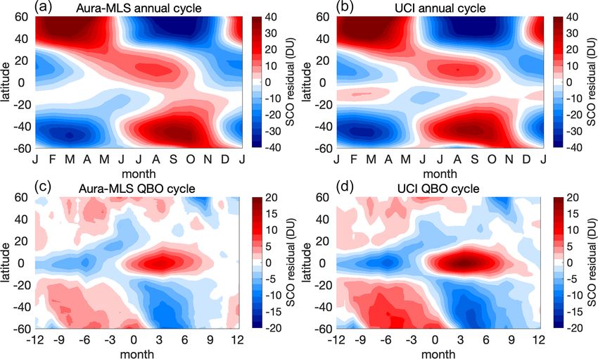
2082                                                              D. J. Ruiz and M. J. Prather: From the middle stratosphere to the surface

Table 1. Summary of key results for the STE flux of O3 and N2 O presented here (in bold).

                                                                    NH                    SH         Global       Notes
       STE O3 flux (TgO3 yr−1 )                                     208                   182            390      IFS Cy38r1; years 1990–2017 (this pa-
                                                                                                                  per; Ruiz et al., 2021)
                                                                    239                   198            437      IFS Cy36r1; years 2000–2007 (Hsu and
                                                                                                                  Prather, 2014)
                                                                    301                   233            534      IFS Cy29r1; years 2000–2006 (Hsu and
                                                                                                                  Prather, 2014)
                                                                    383                   272            655      CMAM; years 1995–2005 (Hegglin and
                                                                                                                  Shepherd, 2009)
       STE N2 O flux (TgN yr−1 )                                     5.1                  6.4           11.5      Years 1990–2017, scaled to 320 ppb
                                                                                                        12.9      Using Aura MLS lifetime of 119 years
                                                                                                                  and 320 ppb
       LMS O3 : N2 O slope∗                                      −23.2                 −17.5                      UCI model
                                                                 −19.4                 −15.3                      ACE-FTS observations
                                                              −23 ± 2               −18 ± 3                       CMAM model; Fig. 13 of Hegglin and
                                                                                                                  Shepherd (2007)
                                                              −22 ± 4               −14 ± 3                       ACE-FTS observations; Hegglin and
                                                                                                                  Shepherd (2007)
                                                                                                      −20.0       Murphy and Fahey (1994)
                                                                                                      −22.0       McLinden et al. (2000)
       STE flux O3 : N2 O (mole mole−1 )                         −23.8                 −16.6                      UCI model as calculated from entries
                                                                                                                  above
                                                                                                      −29.6       CMAM (Hegglin and Shepherd, 2009),
                                                                                                                  using Aura MLS N2 O lifetime
       Best estimate STE O3 flux (Tg yr−1 )            60 % to 50 %          40 % to 50 %         400 ± 60        Current Antarctic ozone hole condi-
                                                                                                                  tions; see text
    ∗ LMS is the lowermost stratosphere only. For the UCI model, months are selected for highest STE (FMAM or February–May in NH; SOND or September–December
    in SH; Fig. 1). For the Canadian Middle Atmosphere Model (CMAM), the monthly ranges from their Fig. 13c and d are estimated. Where no reference is given, the
    source is this paper.

ficient cc > 0.98, except for SH O3 ), indicating that all three                       al., 2021), which will affect tropospheric O3 abundances. It is
enter the troposphere from a seasonally near-uniform mix-                              important to develop observational metrics that test the sea-
ture of O3 : N2O : F11 in the lowermost stratosphere.                                  sonality of the lowermost stratosphere related to STE fluxes
   Global STE peaks in June and reaches a minimum in                                   and to establish monthly STE fluxes as a standard model di-
November. The two hemispheres have dramatically differ-                                agnostic.
ent seasonal amplitudes and somewhat opposite phases. The                                 An interesting result here is the very tight correlation of
NH peak STE for all three species occurs in the late boreal                            the monthly cN2O and cF11 STE, while the O3 STE is some-
spring (May–June), while that in the SH occurs at the start                            times shifted. Loss of N2 O and F11 occurs at very different
of austral spring (September–October). In the NH, O3 STE                               altitudes in the tropical stratosphere (∼ 32 and ∼ 24 km, re-
peaks a month before the c tracers, and in the SH, the whole                           spectively), but both have a similar seasonality in loss, which
annual cycle of O3 is shifted a month earlier. The NH STE                              is driven mostly by the intensity of sunlight along the Earth’s
seasonal amplitude is very large for all species (∼ 4 : 1 ratio                        orbit (N2 O loss peaks in February and reaches a minimum
from max to min), with the exchange almost ceasing in the                              in July; see Fig. 4 from Prather et al., 2015). Photochemi-
fall. In contrast, the SH STE is more uniform year round,                              cal losses of N2 O and F11 drop quickly for air descending
with a 1.5 : 1 ratio for cN2O and cF11 and 2.2 : 1 for O3 .                            from the altitudes of peak loss in the tropics and, hence, the
Other models with similar NH and SH O3 fluxes show dif-                                relative cN2O and cF11 STE fluxes are locked in. O3 , how-
ferent seasonal amplitudes and phasing (see Fig. 6 in Tang et                          ever, continues to evolve photochemically from 24 to 16 km

Atmos. Chem. Phys., 22, 2079–2093, 2022                                                                        https://doi.org/10.5194/acp-22-2079-2022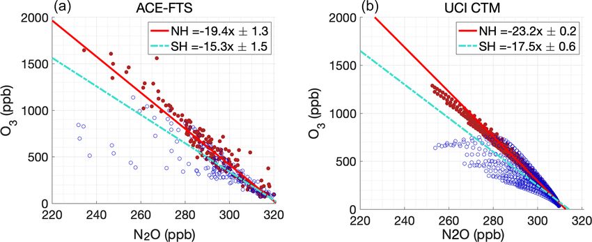
D. J. Ruiz and M. J. Prather: From the middle stratosphere to the surface                                                      2083

                                                                     ports air depleted in N2 O and F11 into the lowermost extra-
                                                                     tropical stratosphere, where it enters the troposphere. R2021
                                                                     showed that the observed surface variability in N2 O from this
                                                                     circulation can be modeled and has a clear QBO signal, but
                                                                     it is one that is not strongly correlated with the QBO signal
                                                                     in stratospheric loss.
                                                                         We generate the IAV of STE fluxes for O3 , cN2O, and
                                                                     cF11 in Fig. 3a, b, and c, with panels for global, NH, and SH.
                                                                     Values are 12-month running means, and so the first modeled
                                                                     point at 1990.5 is the sum of STE for January through De-
                                                                     cember of 1990. In Fig. 3b and c, we also show the seasonal
                                                                     amplitude of STE with double-headed arrows on the left (O3 )
                                                                     and right (cN2O and cF11). In a surprising result, the large
                                                                     NH–SH differences in seasonal amplitude are not reflected
                                                                     in the IAV where NH and SH amplitudes are similar for all
                                                                     three tracers. The QBO modulation of the lowermost strato-
                                                                     sphere and STE appears to be unrelated to the seasonal cycle
                                                                     in STE.
                                                                         Global STE for all three tracers shows QBO-like cycling
                                                                     throughout the 1990–2017 time series. cN2O and cF11 are
                                                                     well correlated (cc ∼ 0.9), but either species with O3 is much
                                                                     less so (cc < 0.7). The hemispheric breakdown provides key
                                                                     information regarding O3 . In the NH, the STE IAV is simi-
                                                                     lar across all three tracers with high correlation coefficients
                                                                     (cc = 0.82 for O3 -cN2O, 0.83 for O3 -cF11, and 0.94 for
                                                                     cN2O-cF11). Conversely, in the SH, O3 STE diverges from
                                                                     the c tracer fluxes, showing opposite-sign peaks in 2003 and
                                                                     2016. The corresponding SH correlations are cc = 0.38, 0.65,
Figure 2. The annual cycle of monthly STE (Tg yr−1 ) of O3 (black    and 0.85. The loss of the correlation between cN2O and
lines), cN2O (orange lines), and cF11 (blue lines). (a) Global STE   cF11 is unusual because cN2O STE drifts downward rela-
fluxes and (b) hemispheric STE fluxes (NH – solid lines; SH –        tive to cF11 STE, particularly after 2007; nevertheless, the
dashed lines). Each month is averaged for the years 1990–2017        fine structure after 2007 is well matched in both tracers.
(e.g., the 28 months of January are averaged). Note the different        In the SH, the massive loss of O3 within the Antarctic
y axes for each tracer in each panel.                                vortex, when mixed with the extra-polar lowermost strato-
                                                                     sphere, will systematically shift the O3 STE to lower values,
                                                                     with less impact on the cN2O and cF11 STE. The IAV of the
(upper boundary of the lowermost stratosphere) through net           Antarctic winter vortex, in terms of the amount of O3 that is
photochemical production in the tropics and loss at mid- and         depleted (see Fig. 4-4 in WMO, 2018), appears to drive the
high-latitudes that depends on sunlight and is thus seasonal.        decorrelation of the SH STE fluxes and is analyzed in Sect. 4.
There may be observational evidence for the patterns mod-                In the NH, the high variability in the Arctic winter strato-
eled here in the correlation of these three tracers in the lower     sphere can modulate the total O3 STE flux (e.g., Hsu and
(16–20 km) and lowermost (12–16 km) extratropical strato-            Prather, 2009) but appears to maintain the same relative ratio
sphere (see Sect. 4).                                                with the cN2O and cF11 fluxes. Model results here indicate
                                                                     that, in the NH, the IAV of O3 , cN2O, and cF11 STE fluxes
3.3   Interannual variability                                        are synchronized, and thus, the air masses entering the low-
                                                                     ermost stratosphere have the same chemical mixtures from
Interannual variability (IAV) of N2 O loss and its lifetime is       year to year. We know that the cold temperature activation
associated primarily with the QBO (most recently, R2021).            of halogen-driven O3 depletion in the Arctic winter at alti-
When the QBO is in its easterly (westerly) phase, the entire         tudes above 400 K (potential temperature) can produce large
overturning circulation is enhanced (suppressed; Baldwin et          IAV in column ozone (Manney et al., 2011), but the magni-
al., 2001). This results in more (less) air rich in N2 O and F11     tude is still much smaller than in the Antarctic, and it may
being transported from the troposphere to the lower or middle        not reach into the lowermost stratosphere (< 380 K potential
stratosphere, thereby increasing (decreasing) the N2 O and           temperature). This model accurately simulates Antarctic O3
F11 sinks (Prather et al., 2015; Strahan et al., 2015). From         loss (Sect. 4), but we have not evaluated it for Arctic loss,
the tropical stratosphere, the overturning circulation trans-        and the Arctic conditions operate closer to the thresholds ini-

https://doi.org/10.5194/acp-22-2079-2022                                             Atmos. Chem. Phys., 22, 2079–2093, 2022
2084 D. J. Ruiz and M. J. Prather: From the middle stratosphere to the surface
tracer transport, by the time they reach the extratropical low-
ermost stratosphere. The overall synchronization of the STE
fluxes implies that the absolute STE flux is driven primarily
by variations in the venting of the lowermost stratosphere as
expected (Holton et al., 1995; Appenzeller et al., 1996) rather
than by variations in the chemistry of the middle strato-
sphere.
This disconnect between the chemical signals generated
by the prominent QBO signature of wind reversals, up-
welling in the tropical stratosphere, and the STE fluxes is
also clear in the magnitude of the loss versus STE. For N2 O,
the IAV of cN2O production has a range of ±0.5 Tg yr−1 ,
whether from the Aura Microwave Limb Sounder (Aura
MLS) observations or the model, whereas the IAV of the
cN2O STE flux is ±1.1 Tg yr−1 . The same is true in relative
terms for cF11. Thus, the modulation of the lowermost strato-
sphere by the QBO is clearly a part of the overall changes
in stratospheric circulation related to the QBO (Tung and
Yang, 1994a; Kinnersley and Tung, 1999) and is the domi-
nant source of IAV for these three greenhouse gases.
3.5 The QBO signal
To examine the QBO cycle in STE flux, we build a compos-
ite pattern (see R2021, Fig. 3, for N2 O surface variations)
by synchronizing the STE IAV in Fig. 2 with the QBO cy-
cle. The sync point (offset equal to 0 months) is taken from
one of the standard definitions of the QBO phase change,
i.e., the shift in sign of the 40 hPa tropical zonal wind from
easterly to westerly (Newman, 2020). The 1990–2017 model
Figure 3. (a) Global STE (Tg yr−1 ), calculated at e90 tropopause, period has 12 QBO cycles, but we restrict our analysis here
of O3 (black line; left y axis), cN2O (orange line; orange right to the years 2001–2016 to overlap with the observed sur-
y axis), and cF11 (blue line; blue right y axis) for the years 1990– face N2 O data. This period includes seven QBO phase tran-
2017. Values are 12-month running means, and so the first point at sitions (January 2002, March 2004, April 2006, April 2008,
1990.5 is the sum of STE for January through December of 1990. August 2010, April 2013, and July 2015), but the observed
(b) NH STE. (c) SH STE. The scales for cN2O and cF11 are kept surface N2 O is highly anomalous during the QBO centered
in a 1 : 2 ratio. The asterisks and vertical double-headed arrows (b,
on August 2010 (R2021), so we remove it from our compar-
c) depict the seasonal mean and amplitude for each species in each
hemisphere.
ison for consistency with R2021 (see their Fig. S4d). The
resulting QBO composites for NH and SH in Fig. 4 span
28 months.
tiating loss where Linoz v3 chemistry may be inadequate. In the NH, the QBO modulation of all three tracers is simi-
The same meteorology and transport model with full strato- lar. The STE flux begins to increase at an offset of −8 months
spheric chemistry is able to simulate Arctic O3 loss (Oslo’s and continues to increase slowly for a year, peaking at an
CTM2; Isaksen et al., 2012), and thus, it will be possible to offset of +4 months; thereafter, it decreases more rapidly in
re-evaluate the NH IAV with such models or with lowermost about one-half of a year (offset equal to +10). The rise-and-
stratosphere tracer measurements. fall cycle takes about 18 months. In the SH, the pattern for
cN2O and cF11 is more sinusoidal and is shifted later by
∼ 3 months. The SH amplitude of the c tracers is slightly
3.4 The link from stratospheric loss to STE flux
larger relative to the hemispheric mean flux than in the NH,
What is unusual about the very tight correlation of cN2O and and thus, the SH QBO signal is larger than the NH by about
cF11 STE fluxes is that the photochemical loss of N2O and 40 %. Thus, over the typical QBO cycle centered on the sync
F11 occurs at very different altitudes in the tropical strato- point, more depleted N2 O and F11 is entering the SH than
sphere, which are not in phase with respect to the QBO, in the NH. For O3 , the SH modulation of STE is irregular
as shown in R2021 (their Fig. 2). The separate phasing of and reduced compared with the NH. Our hypothesis here,
cN2O and cF11 production is lost, presumably by diffusive consistent with the annual cycle of STE (Fig. 1), is that the
Atmos. Chem. Phys., 22, 2079–2093, 2022 https://doi.org/10.5194/acp-22-2079-2022D. J. Ruiz and M. J. Prather: From the middle stratosphere to the surface 2085
surface data. The latitude-by-month pattern of obs-N2 O in-
cludes the impact of both stratospheric loss (∼ 13.5 Tg yr−1 )
and surface emissions (∼ 17 TgN yr−1 ), with the preponder-
ance of emissions being in the NH (Tian et al., 2020). Total
emissions are not expected to have large IAV but may have a
seasonal cycle. The seasonal variation in the surface N2 O can
also be driven by seasonality in the interhemispheric mixing
of the NH–SH gradient (∼ 1 ppb).
4.1 Annual cycle
Figure 5 replots the hemispheric mean annual cycles of
cN2O STE flux alongside the annual cycles of surf-N2O
and obs-N2 O. As noted above, the STE in each hemisphere
Figure 4. QBO composites of the STE of O3 (black lines; left is almost in opposite phase, as is the modeled surf-N2O
y axes), cN2OX (orange lines; orange right y axes), and cF11X (taken from Fig. 5 in R2021). The NH : SH amplitude ratio
(blue lines; blue right y axes) for the (a) NH (0–90◦ N; solid lines) is about 2.4 : 1 for both STE and surf-N2O. The lag from
and (b) SH (0–90◦ S; dashed lines). These composites are averages the peak STE flux of cN2O (negative N2 O) to minimum
centered on the QBO phase transition at 40 hPa throughout the pe-
surf-N2O is about 3 months. Such a 90◦ phase shift is ex-
riod of surface observations (years 2001–2016, excluding the Au-
gust 2010 observed anomaly, for a total of six QBOs). Note that the
pected for the seasonal variation in a long-lived tracer rela-
y axes limits are different for each panel, but the interval scale is tive to a seasonal source or sink. The time lag between the
consistent for each tracer. signal at the tropopause and at the surface, the tropospheric
turnover time, should be no more than a month. Surprisingly,
the cN2O STE seasonal amplitude is much larger in the NH
breakup of the Antarctic ozone hole has a major impact on (±3.4 Tg yr−1 ) than in the SH (±1.3 Tg yr−1 ), although the
STE, particularly that of O3 , and that its signal has a large SH mean (6.5 Tg yr−1 ) is larger than the NH (5.2 Tg yr−1 ).
IAV that does not synchronize with the QBO. Surprisingly, Essentially, there is more variability in air depleted in N2 O
the large wintertime IAV in the NH Arctic, in the form of entering the NH, but air entering the SH has a larger overall
sudden stratospheric warmings, does not seem to have a ma- deficit. Thus, in our model, the stratosphere creates a NH–
jor role in STE fluxes as noted above. This model may miss SH gradient of +0.3 ppb at the surface, which is a signifi-
some of the Arctic O3 depletion, but it accurately simulates cant fraction of the observed the N–S difference of +1.3 ppb
the warmings, which must have a small impact on STE be- (R2021). This important result needs to be verified with other
cause they do not disrupt the clear QBO signal in the c trac- models or analyses because it constrains the NH–SH location
ers. of sources.
In the NH, as noted in R2021, the two surface abundances,
4 Surface variability in N2 O related to STE flux surf-N2O and obs-N2 O, have the same amplitude and phase,
implying that, if the model is correct, the emissions-driven
The surface variability in N2 O is driven by surface emissions, surface signal has no seasonality, although we know that
stratospheric loss, and atmospheric transport that mixes the some important emissions are seasonal (Butterbach-Bahl et
first two signals. R2021 explored the variability originat- al., 2013). In the SH, the surf-N2O signal is much smaller,
ing only from stratospheric chemistry using the decaying in parallel with the small seasonal amplitude in cN2O STE,
tracer N2OX. Here, we use surf-N2O to denote the surface but it is out of phase with the obs-N2 O. This result implies
abundances of N2OX when corrected to steady state. R2021 that the SH has some highly seasonal sources, or simply that
showed that three independent chemistry transport models the forcing of SH surf-N2O by the seasonal cycle of cN2O
produced annual and QBO patterns in surface N2 O simply is weak. Indeed, this is what we might expect from Fig. 3. In
from stratospheric loss. In this paper, we link surf-N2O to the NH, the seasonal amplitude in N2 O overwhelms the IAV
the STE cN2O flux, which is linked above to the STE O3 amplitude and is driving the obs-N2 O, but in the SH, both
flux. amplitudes are comparable. Given the quasi-regular nature
The observed surface N2 O, denoted as obs-N2 O and taken of the QBO, it would interfere with the seasonal cycle and
from the NOAA network (Dlugokencky et al., 2019), shows likely change its phase (as found for other models in R2021).
a slowly increasing abundance (∼ 0.9 ppb yr−1 ) with a clear In the NH, the annual cycle of O3 and cN2O STE are
signal of annual and interannual variability at some latitudes clearly linked. If we accept that the obs-N2 O NH seasonal
(see R2021). We calculate the annual and QBO-composite cycle is simply driven by the STE flux, then how will tro-
obs-N2 O after detrending and restrict the analysis in this sec- pospheric O3 respond seasonally? A mole fraction scaling
tion to the model years 2001–2016 to be consistent with the of the STE fluxes gives an O3 : N2 O ratio of ∼ 25, and thus,
https://doi.org/10.5194/acp-22-2079-2022 Atmos. Chem. Phys., 22, 2079–2093, 20222086 D. J. Ruiz and M. J. Prather: From the middle stratosphere to the surface
Figure 6. (a) NH and (b) SH QBO composites of cN2O STE flux
(Tg yr−1 ; orange lines, left axis; Fig. 4) and surf-N2O and obs-N2 O
(ppb; red and blue knotted lines, right axes; see Fig. 3 in R2021).
Figure 5. The annual cycle of O3 and cN2O STE (black and orange
Results are shown for the years 2001–2016 (six QBO phase transi-
lines; left y axes) and the surf-N2O and obs-N2 O (red and blue tions; see Fig. 4). The surf-N2O data are from UCI CTM, and obs-
knotted lines; right y axes) taken from R2021 (see their Fig. 5) for N2 O are taken from NOAA ESRL (Earth System Research Labora-
the (a) NH and (b) SH. cN2O, surf-N2O, and obs-N2 O have been tory; see the text).
rescaled to reflect that of a tropospheric abundance of 320 ppb. The
hemispheric domains for STE are defined as 0–90◦ , while the surf-
N2O and obs-N2 O domain is from 30–90◦ N/S. Note that the left
y axes limits are different between the tracers, but the interval scale ing. This ratio is larger than the corresponding one from the
is the same. annual cycles (∼ 0.1 ppb/Tg yr−1 ) because the length of the
QBO cycle leads to longer accumulation of N2 O-depleted air
from the cN2O flux.
scaling the surf-N2O amplitude gives a large O3 surface sea- In the SH, where the QBO cycle in cN2O flux has a large
sonality of ∼ 18 ppb. However, the residence time of a tro- amplitude, the modeled surf-N2O matches obs-N2 O in am-
pospheric O3 perturbation is ∼ 1 month, and thus, the peak plitude and phase as reported in R2021. In the NH, the com-
surface abundance will lag the peak STE flux by only about parison of surf-N2O with obs-N2 O is not so good; obs-N2O
a month and not by 3 months as for N2 O. O3 will equili- has a much smaller amplitude and a different phase. This
brate with the flux on monthly timescales and not accumu- QBO cycle pattern is similar, but reversed, to that of the an-
late. Thus, our estimate is that NH 30–90◦ surface ozone nual cycle and can be understood in the same way. The NH
might increase about 5 ppb, peaking in June, due to the STE QBO cycle has a relatively small amplitude, and thus, the in-
flux. In the SH, seasonal patterns are weaker and not well terference with the large-amplitude annual cycle adds noise,
defined, and thus, no obvious STE O3 signal is expected. obscuring the QBO cycle. In the SH it is the opposite, with
its weak annual cycle, and the SH QBO cycle is clear. The
4.2 QBO cycle modeled cN2O fluxes enable us to understand the large-scale
variability in the observations.
The QBO composite of hemispheric mean cN2O STE flux Thus, for both annual and QBO fluctuations, when the
from Fig. 4 is compared with the composite of surface abun- variation in the STE flux is dominated by either cycle, the
dances (surf-N2O and obs-N2 O) in Fig. 6. The peak in cN2O surface variations are clearly seen and modeled for that cy-
flux is broad and flat, but it centers on +2 months for the NH cle. This further supports the findings in R2021, and other
and +4 months for the SH. Unlike the annual cycle, the QBO studies, that hemispheric surface N2 O variability is driven by
cycle in STE flux is almost in phase in both hemispheres, stratospheric loss on annual (NH) and QBO (SH) cycles, and
with the NH preceding the SH. This phasing of the QBO cy- it is clearly tied to the STE flux. Given the connection be-
cle in surface N2 O was seen with the three models in R2021. tween O3 and cN2O STE, this relational metric can be used
In both hemispheres, the modeled surf-N2O peaks before the to constrain the O3 STE for a model ensemble.
rise in cN2O and then decreases through most of the period,
with elevated cN2O flux as expected. The amplitude of the
QBO STE flux is smaller in the NH than SH by about half, 5 Lowermost stratosphere
and the amplitude of surf-N2O is likewise smaller. The ratio
of the amplitudes of surf-N2O to cN2O STE flux is similar If we accept that matching the observed annual and QBO cy-
in both hemispheres (∼ 0.4 ppb/Tg yr−1 ), which is encourag- cles in surface N2 O constrain the modeled STE cN2O flux,
Atmos. Chem. Phys., 22, 2079–2093, 2022 https://doi.org/10.5194/acp-22-2079-2022D. J. Ruiz and M. J. Prather: From the middle stratosphere to the surface 2087
then how can we use that to also constrain the modeled STE In the modeled SH (Fig. 7b), one can see strings of points
O3 flux? All evidence, theoretical, observational, and mod- that are samples along neighboring cells and reflect a linear
eled, shows that the STE flux is simultaneous for all species mixing line between two different endpoints, one of which
(e.g., Fig. 1) and in proportion to their relative abundances has experienced extensive O3 depletion (i.e., the Antarctic
(i.e., tracer : tracer slopes) in the lowermost stratosphere, de- O3 hole). We know that there is some chemical loss of O3 in
fined roughly as the region at 100–200 hPa in each hemi- the NH lowermost polar stratosphere during very cold win-
sphere outside the tropics (Plumb and Ko, 1992). ters (Manney et al., 2011; Isaksen et al., 2012), but it is not
extensive enough to systematically affect the O3 : N2 O slope
over the mid-latitude lowermost stratosphere in either the
5.1 The O3 : N2 O slopes and STE fluxes ACE observations or the CTM simulations.
We can test the Plumb and Ko (1992) hypothesis in our 5.2 IAV of the Antarctic ozone hole and the SH STE O3
model framework by comparing the relative STE fluxes for flux
O3 , cN2O, and cF11 with the modeled tracer–tracer slopes
in the lowermost stratosphere. These slopes can then be The Antarctic ozone hole appears to be the source of the NH–
tested using SCISAT-1 ACE-FTS (Scientific Satellite-1 At- SH asymmetry in the STE fluxes of O3 versus N2 O. It is
mospheric Chemistry Experiment Fourier transform spec- known that the massive chemical depletion of O3 inside the
trometer) measurements of O3 and N2 O in the lowermost Antarctic vortex between about 13 and 23 km altitude creates
stratosphere to establish the ratio of the two STE fluxes. The an air mass with lower O3 : N2 O ratios than usually found
ACE-FTS O3 : N2 O slopes were used for model transport in the mid-latitude lowermost stratosphere. When the vor-
and chemistry evaluation (Hegglin and Shepherd, 2007) and tex breaks up, nominally in late November, much of this O3 -
found to be very sensitive to satellite sampling, except in the depleted air can mix along isentropes into the mid-latitude
lowermost stratosphere. lowermost stratosphere, changing the O3 : N2 O ratios and re-
Figure 7a and b show the N2 O-O3 slope in each hemi- ducing the SH STE O3 flux.
sphere taken from the ACE climatology dataset and the UCI We have additional information on the SH O3 STE flux
CTM. The current ACE dataset (version 3.5) has been cu- from the year-to-year variations in the size of the ozone hole.
rated from measurements made by ACE-FTS from Febru- The best measure of the scale of Antarctic ozone depletion
ary 2004 to February 2013 (Koo et al., 2017). The SCISAT is the October mean ozone column (DU) averaged from the
orbit results in irregular season–latitude coverage, and thus, pole to 63◦ S equivalent latitude (see Figs. 4–5 in WMO,
we average the lowermost stratosphere data over a wide 2018). When we compare the CTM with the observations
range of latitudes centered on the peak STE flux (20–60◦ (Fig. 8), we find remarkable verisimilitude in the model be-
in both hemispheres). For both ACE data and the CTM, we cause the root mean squared difference is 9 DU out of a stan-
keep to the lowermost stratosphere (200–100 hPa) and aver- dard deviation of 29 DU, and the correlation coefficient is
age over the 4-month peak of STE flux (February–May in the 0.96. Thus, we have confidence that we are simulating the
NH and September–December in the SH; see Fig. 1). Extend- correct IAV of the ozone hole. Next, we plot the modeled O3
ing into the upper tropical troposphere at 20◦ helps define the STE flux (summed over the 12 months following the peak
tropospheric endpoint of the slope (low O3 ; high N2 O). Our ozone hole; November–October) with the modeled October
method described here for deriving the slopes from the ACE- ozone column and find a fairly linear relationship. If we es-
FTS data is slightly different from that of Hegglin and Shep- timate the STE O3 flux before the O3 hole, when the mean
herd (2007; e.g., we do not anchor the tropospheric point), October O3 column was about 307 DU, then our O3 flux in-
and we have the advantage of a longer record. creases to 209 Tg yr−1 (see Fig. 8; red marker), eliminating
Based on the long-term mean STE fluxes in the model, we the hemispheric asymmetry in O3 STE flux.
would expect an O3 : N2 O slope of about −24 (parts per bil- The annual deficit in SH STE O3 flux brought on by the
lion of O3 per part per billion of N2 O; hereafter ppb ppb−1 ) Antarctic ozone hole ranges from about 5 to 55 Tg yr−1 and
in the NH and −17 in the SH. The slopes fitted to our mod- with a central value of 30 Tg yr−1 or 14 % of the total. Us-
eled grid cell values of O3 and N2O in the lowermost strato- ing the decadal trends 1965–2000 from Hegglin and Shep-
sphere are remarkably similar, with −23.2 (NH) and −17.5 herd (2009), this deficit is 8 %, and from Meul et al. (2018),
(SH). The ACE data are more scattered but show similar, it is 5 %. Since both of these models calculate a much larger
smaller slopes of −19.4 (NH) and −15.3 (SH). Thus, the SH flux (∼ 300 Tg yr−1 ), we estimate their absolute change
NH–SH asymmetry in O3 versus N2 O STE fluxes is clearly in O3 flux to be 24 and 15 Tg yr−1 , respectively. Because
reflected in the tracer–tracer slopes, for both modeled and the ozone hole effectively removes a fixed, rather than pro-
observed values. Hegglin and Shepherd (2007) had already portional, amount of ozone that presumably is mapped onto
identified these NH : SH differences when comparing their the STE flux the following year, we believe the absolute
model to the ACE-FTS observations (their Fig. 13c, d), but change is the best measure. Thus, the three models estimate
implications for STE fluxes were not brought forward. the ozone hole causes a deficit in the SH O3 STE flux in the
https://doi.org/10.5194/acp-22-2079-2022 Atmos. Chem. Phys., 22, 2079–2093, 20222088 D. J. Ruiz and M. J. Prather: From the middle stratosphere to the surface
Figure 7. O3 versus N2 O (x axis) scatterplots from (a) SCISAT ACE-FTS and (b) the UCI CTM. ACE-FTS data are from monthly cli-
matologies for the period February 2004 to February 2013, restricted to 200–100 hPa, with latitudes of about 20–60◦ and the months of
February–May (NH; red) or September–December (SH; blue). The linear fit lines (ppb ppb−1 ; values in the legend) are restricted to larger
N2 O values (> 280 ppb) to more accurately represent the STE fluxes (see Olsen et al., 2001).
range of 15–30 Tg yr−1 . The UCI CTM’s ability to match the
observed IAV of the ozone hole and to match that linearly
with the deficit in STE flux provides support for the upper
end of the range. Note that the difference in O3 : N2 O slopes
between NH and SH in Fig. 7 is about 5. If we attribute that
solely to the ozone hole and split the flux of N2 O-depleted air
evenly between hemispheres, then the ozone-hole-driven O3
STE flux difference is about 55 Tg yr−1 , which is about twice
that derived from the variability in our model. This difference
in estimated flux indicates that, even without chlorine-driven
ozone depletion, the O3 : N2 O slopes may be inherently dif-
ferent simply because of the strong descent inside the winter-
time Antarctic vortex. This can be readily investigated with
further model studies.
We looked for any relationship between ozone hole IAV Figure 8. Interannual variability in the observed Antarctic ozone
and the STE fluxes of cN2O or cF11 and found mostly a scat- hole from 1990 to 2017 (blue dots; left y axis) versus the CTM-
terplot with no clear relationship. Given the analysis above, modeled ozone hole (x axis); plus the CTM-modeled SH STE
we expect that much of the scatter is related to QBO cycles. O3 flux (black dots; right y axis) versus the modeled ozone hole
(x axis). The ozone hole is measured by the total ozone column
(DU) averaged daily over October, poleward of 63◦ S in equiva-
5.3 Other model–measurement metrics related to STE
lent latitude (see Fig. 4.5 in WMO, 2018). The SH STE O3 flux
What else might affect O3 STE? Stratospheric column O3 (Tg yr−1 ) is centered on 1 May of the following year (i.e., the
(DU) varies on annual and QBO timescales. These changes 12 months following the nominal breakup of the ozone hole). The
black line is a simple regression fit of the modeled STE to the mod-
in O3 overhead can have a direct influence on O3 transport to
eled ozone hole (black dots), and the red dot is our estimate of pre-
the troposphere, but the link requires further analysis. Tang
ozone-hole SH STE O3 flux based on the observed 1979–1982 O3
et al. (2021) showed the UCI CTM is able to capture the ob- column.
served annual cycle of stratospheric O3 column as extracted
from total column, using the Ziemke et al. (2019) method.
QBO modulation of stratospheric column O3 has not been 6 Conclusions
fully investigated since Tung and Yang (1994b). Yet, the fluc-
tuations in mass over the annual cycle are comparable to the This work examines how closely O3 STE is linked to STE
corresponding variability in O3 STE flux (1 DU = 10.9 Tg) fluxes of other trace gases. By including our complemen-
and likely connected (Fig. 9). tary N2 O and F11 tracers, we can follow the stratospheric
loss of these gases along with stratospheric O3 across the
tropopause. The magnitudes of the fluxes are proportional
to their abundances in the lower stratosphere, as expected
(Plumb and Ko, 1992), and their variability is highly corre-
Atmos. Chem. Phys., 22, 2079–2093, 2022 https://doi.org/10.5194/acp-22-2079-2022D. J. Ruiz and M. J. Prather: From the middle stratosphere to the surface 2089 Figure 9. Stratospheric O3 column residuals taken from Aura MLS (a, c) and UCI CTM (b, d), for their mean annual cycle (a, b) and mean QBO cycle (c, d), during the years 2005–2017. Residuals are defined at each latitude with a mean of 0 DU. lated with one another, indicating that they are entering the STE flux, we calculate that the O3 : N2 O slope in the lower- troposphere simultaneously. Even the distinct QBO pattern most stratosphere should average to −30. We conclude that of STE fluxes is consistent across O3 , N2 O, and F11. We their diagnosis of the STE O3 flux, 655 Tg yr−1 , is inconsis- further constrain the N2 O transport pathway by linking STE tent with the circulation that generated the O3 : N2 O slopes of depleted N2 O air with surface fluctuations of N2 O abun- and is 50 % too large. We do not view this as a critical assess- dance. The surface response in modeled N2 O matches well ment of CMAM, since it involves us combining diagnostics with the observed surface variability in the SH, indicating from two separate publications and possibly different model that surface variability is driven largely by STE flux. simulations, but it is an example of how we might expect fu- Consistency of STE O3 flux. As summarized here, there are ture studies of the STE O3 flux to self-evaluate. a number of model diagnostics and observational constraints Uncertainty Quantification in STE O3 flux. Deriving a best that provide a reality check on the consistency of the modeled estimate and uncertainty from this work involves expert judg- O3 STE flux. In Table 1, we examine these for our model ment. Changes in meteorological data used by the UCI CTM and also for the CMAM model (Hegglin and Shepherd, (IFS cycles 29r1, 36r1, and 38r1, all at 60-layer 1.1◦ resolu- 2007, 2009) because it is one of the few with enough pub- tion; see Table 1) give a standard deviation in STE of 13 % lished results. For UCI, we calculate NH : SH fluxes of O3 (only 3 values). If we use observations to derive a value, as in (208 : 182 Tg-O3 yr−1 ) and N2 O (5.1 : 6.4 Tg-N yr−1 ). Thus Murphy and Fahey (1994), we must expand our dimensions the mole fraction slopes in the lowermost stratosphere should to the uncertainty in the NH : SH split of N2 O flux to cal- be −23.8 (NH) and −16.6 (SH). Our model O3 : N2 O slopes culate each hemisphere’s O3 flux. The factors are as follows: are −23.2 (NH) and −17.5 (SH). Given the seasonal vari- (1) total STE N2 O flux is 12.9 Tg-N yr−1 from the Aura MLS ability and scatter in the correlation plots (Fig. 7), we count data, and we assign a ±10 % 1σ uncertainty; (2) the NH : SH this as consistent. For CMAM, the modeled O3 : N2 O slopes, split of the N2 O flux is 44 : 56 in our current model, and was −23 ± 2 (NH) and −18 ± 3 (SH), are similar to ours and not diagnosed for previous ones, and so we assume a value also to the ACE-FTS observations as analyzed by Hegglin of 50 : 50 that ranges from 40 : 60 to 60 : 40; (3) analysis of and Shepherd (2007), with −22 ± 4 (NH) and −14 ± 3 (SH) the ACE-FTS observations (ours and Hegglin and Shepherd, or, by us, −19 (NH) and −15 (SH). CMAM does not report 2007) gives O3 : N2 O slopes of about −21 (NH) and −15 the implied STE N2 O fluxes derived from their photochem- (SH) to which we assign a 1σ uncertainty of ±3. Propagat- ical loss of N2 O, but their model seems to match observa- ing these as root mean square errors, we find a ±15 % uncer- tions of N2 O in the middle stratosphere, and so we assume tainty in the global value, i.e., 400 ±60 Tg yr−1 . Uncertainty that the Aura-MLS-derived N2 O fluxes are a close estimate in the hemispheric values is more difficult to assess, and from (12.9 Tg-N yr−1 ). Note that we are using Aura MLS N2 O a range of model results shown in Table 1, we can only es- values here to calculate the photochemical loss, which oc- timate that the NH : SH ratio is between 60 : 40 and 50 : 50, curs in the middle to upper stratosphere (see R2021 for the which is a range that bounds our and CMAM results plus methodology). Just using the CMAM global numbers for O3 2 %. Note that this estimate is for current conditions with https://doi.org/10.5194/acp-22-2079-2022 Atmos. Chem. Phys., 22, 2079–2093, 2022
2090                                                                D. J. Ruiz and M. J. Prather: From the middle stratosphere to the surface

Table 2. Metrics from measurements or constrained values for chemistry–climate models (CCMs) related to the stratosphere–troposphere
exchange.

  Name                      Metric                            Measured values                    Model requirements                  Example figure
  N2 O loss                 Annual and QBO cycles             Monthly N2 O loss calcu-           Stratospheric chemistry for N2 O    Fig. 4 (Prather et al.,
                            of global mean                    lated from Aura MLS                as tracer; a QBO cycle; monthly     2015); Fig. 2 (Ruiz et al.,
                            stratospheric N2 O loss           profiles (2005–present)            mean diagnostics                    2021); Fig. 3 (this paper)
  STE slopes                Matching O3 : N2 O                ACE FTS profiles                   Stratospheric O3 and N2 O           Fig. 7 (this paper)
                            slopes in lowermost               (2004–2013)                        calculation (possibly also
                            stratosphere                                                         CFCs); monthly snapshots
  Stratospeheric O3         Annual and QBO com-               Monthly zonal mean strato-         Stratospheric O3 chemistry; a       Fig. 9 (this paper)
  column                    posite cycles of                  spheric O3 column from             QBO cycle; monthly mean di-
                            stratospheric O3 column           Ziemke et al. (2019)               agnostics; separate stratosphere
                                                              (2005–present)                     and troposphere O3 columns
  N2 O loss at              Annual and QBO                    NOAA surface N2 O                  Stratospheric N2 O chemistry;       Fig. 3 (Ruiz et al., 2021);
  surface                   composite cycles of               observations                       N2OX as a tracer; monthly mean      Fig. 5 (this paper)
                            surface N2 O solely from                                             diagnostics
                            stratospheric loss
                                                              Constrained (modeled)
                                                              values
  STE flux of O3                                              Monthly, latitude, or              Run O3 stratosphere as a tracer;    Figs. 1 and 2 (this paper)
                                                              hemispheric resolved;              diagnose monthly flux into
                                                              net O3 flux                        troposphere, at tropopause or
                                                                                                 through tropospheric loss of O3
                                                                                                 stratosphere
  STE flux of N2 O                                            Monthly, latitude, or              Run cN2O (cF11) as a tracer; di-    Figs. 1 and 2 (this paper);
  depleted air (also                                          hemispheric resolved; STE          agnose monthly flux into tropo-
  CFC-11)                                                     flux of N2 O (CFC-11)              sphere
  SH O3 hole and                                              Change in SH O3 STE flux           IAV of ozone hole; daily total O3   Fig. 7 (this paper)
  flux                                                        with size of ozone hole;           column (lat, long); monthly SH
                                                              observed IAV of O3 hole            O3 STE flux

Note: constrained values are the model-only derived quantities that can be diagnosed from CCMs or CTMs.

a regularly occurring Antarctic ozone hole. We believe the                               stratosphere would be needed to overturn the established the-
low 50 : 50 ratio is plausible because we have shown that                                ory. Our work reemphasizes the importance of trace gas cor-
our large SH STE N2 O flux is consistent with the surface                                relations in the lowermost stratosphere as a key observational
QBO variability in N2 O. For years pre-1980, and for when                                metric for climate models that may be able to constrain to-
the ozone hole recovers later this century, we anticipate that                           tal STE fluxes. The tracer slopes may go beyond just relative
the SH O3 : N2 O slope will revert to −18 to −21 and the total                           STE fluxes because we have other measurements from the
STE O3 flux to 430–460 Tg yr−1 . This simplistic estimate is                             upper stratosphere to the surface that constrain, for example,
based on a fixed atmospheric circulation.                                                the absolute flux of N2 O better than we first did using just
   A major surprise from our model is that the STE flux                                  the modeled lifetime.
of O3 is predominantly NH biased currently and only be-                                     In Table 2, we gather a set of observation-based model
cause of the Antarctic ozone hole. Prior to 1980, and after                              metrics that relate to STE fluxes and will help the commu-
2060, it would/will be symmetric between the hemispheres.                                nity build more robust models to better derive the STE flux
Our model calculates slightly greater STE fluxes for trace                               of O3 .
gases like N2 O or F11 in the SH, which is counter to the
prevailing theory that the wave-driven fluxes force relatively
greater STE in the NH. This difference cannot be directly                                Code and data availability. MATLAB code was used to analyze
tested with observations of trace gases, but a range of N2 O                             the data and generate the figures and tables in this work. This code,
hemispheric observations are well modeled and support this                               together with the underlying data used in this work, can be accessed
premise. More extensive work with multi-model ensembles                                  through the Dryad repository at https://doi.org/10.7280/D1JX0K
                                                                                         (Ruiz, 2021).
that include both chemical and dynamical diagnostics in the

Atmos. Chem. Phys., 22, 2079–2093, 2022                                                                      https://doi.org/10.5194/acp-22-2079-2022
D. J. Ruiz and M. J. Prather: From the middle stratosphere to the surface 2091
Author contributions. DJR and MJP designed and carried out Mole Fractions from the NOAA ESRL Carbon Cycle Cooper-
the study and prepared the paper for publication. ative Global Air Sampling Network, 1997–2018, Version: 2019-
07, https://doi.org/10.15138/53g1-x417, 2019.
Gettelman, A., Holton, J. R., and Rosenlof, K. H.: Mass fluxes of
Competing interests. The contact author has declared that nei- O3 , CH4 , N2 O and CF2 Cl2 in the lower stratosphere calculated
ther they nor their co-author has any competing interests. from observational data, J. Geophys. Res.-Atmos., 102, 19149–
19159, https://doi.org/10.1029/97jd01014, 1997.
Griffiths, P. T., Murray, L. T., Zeng, G., Shin, Y. M., Abraham, N.
Disclaimer. Publisher’s note: Copernicus Publications remains L., Archibald, A. T., Deushi, M., Emmons, L. K., Galbally, I.
neutral with regard to jurisdictional claims in published maps and E., Hassler, B., Horowitz, L. W., Keeble, J., Liu, J., Moeini, O.,
institutional affiliations. Naik, V., O’Connor, F. M., Oshima, N., Tarasick, D., Tilmes, S.,
Turnock, S. T., Wild, O., Young, P. J., and Zanis, P.: Tropospheric
ozone in CMIP6 simulations, Atmos. Chem. Phys., 21, 4187–
4218, https://doi.org/10.5194/acp-21-4187-2021, 2021.
Acknowledgements. We thank Xin Zhu, at UCI, for her help in
Hamilton, K. and Fan, S. M.: Effects of the stratospheric
generating the UCI CTM simulations. We gratefully acknowledge
quasi-biennial oscillation on long-lived greenhouse gases in
the work of the MLS team in producing the level 3 datasets that
the troposphere, J. Geophys. Res.-Atmos., 105, 20581–20587,
enabled our MLS-related analyses. Work at the Jet Propulsion Lab-
https://doi.org/10.1029/2000jd900331, 2000.
oratory, California Institute of Technology, was performed under
Hegglin, M. I. and Shepherd, T. G.: O3 -N2 O correlations from the
contract with the National Aeronautics and Space Administration.
Atmospheric Chemistry Experiment: Revisiting a diagnostic of
We thank the ACE-FTS team, for making the climatology data used
transport and chemistry in the stratosphere, J. Geophys. Res.-
here available for our analyses. The Atmospheric Chemistry Ex-
Atmos., 112, D19301, https://doi.org/10.1029/2006jd008281,
periment (ACE), also known as SCISAT, is a Canadian-led mission
2007.
mainly supported by the Canadian Space Agency. We also acknowl-
Hegglin, M. I. and Shepherd, T. G.: Large climate-induced changes
edge Ed Dlugokencky, for providing the surface N2 O data that were
in ultraviolet index and stratosphere-to-troposphere ozone flux,
used here to produce an observation-based reference with which to
Nat. Geosci., 2, 687–691, https://doi.org/10.1038/Ngeo604,
compare our simulated results.
2009.
Hess, P., Kinnison, D., and Tang, Q.: Ensemble simulations of the
role of the stratosphere in the attribution of northern extratropical
Financial support. The research at UCI has been supported tropospheric ozone variability, Atmos. Chem. Phys., 15, 2341–
by grants from the National Aeronautics and Space Admin- 2365, https://doi.org/10.5194/acp-15-2341-2015, 2015.
istration’s Modeling, Analysis, and Prediction (MAP) Program Hirsch, A. I., Michalak, A. M., Bruhwiler, L. M., Peters,
(grant no. NNX13AL12G), the Atmospheric Chemistry Model- W., Dlugokencky, E. J., and Tans, P. P.: Inverse mod-
ing and Analysis Program (ACMAP; grant nos. 80NSSC20K1237 eling estimates of the global nitrous oxide surface flux
and NNX15AE35G), and the National Science Foundation (grant from 1998–2001, Global Biogeochem. Cy., 20, Gb1008,
no. NRT-1633631). https://doi.org/10.1029/2004gb002443, 2006.
Holton, J. R.: On the Global Exchange of Mass be-
tween the Stratosphere and Troposphere, J. At-
Review statement. This paper was edited by Jens-Uwe Grooß mos. Sci., 47, 392–395, https://doi.org/10.1175/1520-
and reviewed by two anonymous referees. 0469(1990)0472.0.Co;2, 1990.
Holton, J. R., Haynes, P. H., Mcintyre, M. E., Douglass, A. R.,
Rood, R. B., and Pfister, L.: Stratosphere-Troposphere Exchange,
References Rev. Geophys., 33, 403–439, 1995.
Hsu, J. and Prather, M. J.: Stratospheric variability and tro-
Appenzeller, C., Holton, J. R., and Rosenlof, K. H.: Seasonal vari- pospheric ozone, J. Geophys. Res.-Atmos., 114, D06102,
ation of mass transport across the tropopause, J. Geophys. Res.- https://doi.org/10.1029/2008jd010942, 2009.
Atmos., 101, 15071–15078, https://doi.org/10.1029/96JD00821, Hsu, J. and Prather, M. J.: Global long-lived chemical modes ex-
1996. cited in a 3-D chemistry transport model: Stratospheric N2 O,
Baldwin, M. P., Gray, L. J., Dunkerton, T. J., Hamilton, K., Haynes, NOy , O3 and CH4 chemistry, Geophys. Res. Lett., 37, L07805,
P. H., Randel, W. J., Holton, J. R., Alexander, M. J., Hirota, I., L07805, https://doi.org/10.1029/2009gl042243, 2010.
Horinouchi, T., Jones, D. B. A., Kinnersley, J. S., Marquardt, C., Hsu, J. N. and Prather, M. J.: Is the residual vertical ve-
Sato, K., and Takahashi, M.: The quasi-biennial oscillation, Rev. locity a good proxy for stratosphere-troposphere ex-
Geophys., 39, 179–229, 2001. change of ozone?, Geophys. Res. Lett., 41, 9024–9032,
Butterbach-Bahl, K., Baggs, E. M., Dannenmann, M., Kiese, https://doi.org/10.1002/2014GL061994, 2014.
R., and Zechmeister-Boltenstern, S.: Nitrous oxide emis- Hsu, J., Prather, M. J., and Wild, O.: Diagnosing the
sions from soils: how well do we understand the processes stratosphere-to-troposphere flux of ozone in a chemistry
and their controls?, Philos. T. R. Soc. B, 368, 20130122, transport model, J. Geophys. Res.-Atmos., 110, D19305,
https://doi.org/10.1098/rstb.2013.0122, 2013. https://doi.org/10.1029/2005jd006045, 2005.
Dlugokencky, E. J., Crotwell, A. M., Mund, J. W., Crotwell, M.
J., and Thoning, K. W.: Atmospheric Nitrous Oxide Dry Air
https://doi.org/10.5194/acp-22-2079-2022 Atmos. Chem. Phys., 22, 2079–2093, 2022You can also read