Geolectric field measurement, modelling and validation during geomagnetic storms in the UK
←
→
Page content transcription
If your browser does not render page correctly, please read the page content below
J. Space Weather Space Clim. 2021, 11, 37
Ó British Geological Survey, UKRI. Published by EDP Sciences 2021
https://doi.org/10.1051/swsc/2021022
                                                                                                                                     Available online at:
Topical Issue - Geomagnetic Storms and Substorms:                                                                                   www.swsc-journal.org
a Geomagnetically Induced Current perspective

 RESEARCH ARTICLE                                                                                                                OPEN          ACCESS

Geolectric field measurement, modelling and validation during
geomagnetic storms in the UK
Ciarán D. Beggan*, Gemma S. Richardson, Orsi Baillie, Juliane Hübert, and Alan W. P. Thomson
British Geological Survey, Research Ave South, Riccarton, EH14 4AP Edinburgh, UK

              Received 26 June 2020 / Accepted 25 May 2021

              Abstract – Significant geoelectric fields are produced by the interaction of rapidly varying magnetic fields
              with the conductive Earth, particularly during intense geomagnetic activity. Though usually harmless, large
              or sustained geoelectric fields can damage grounded infrastructure such as high-voltage transformers and
              pipelines via geomagnetically induced currents (GICs). A key aspect of understanding the effects of space
              weather on grounded infrastructure is through the spatial and temporal variation of the geoelectric field.
              Globally, there are few long-term monitoring sites of the geoelectric field, so in 2012 measurements of
              the horizontal surface field were started at Lerwick, Eskdalemuir and Hartland observatories in the UK.
              Between 2012 and 2020, the maximum value of the geoelectric field observed was around 1 V/km in
              Lerwick, 0.5 V/km in Eskdalemuir and 0.1 V/km in Hartland during the March 2015 storm. These
              long-term observations also allow comparisons with models of the geoelectric field to be made. We use
              the measurements to compute magnetotelluric impedance transfer functions at each observatory for periods
              from 20 to 30,000 s. These are then used to predict the geoelectric field at the observatory sites during
              selected storm times that match the recorded fields very well (correlation around 0.9). We also compute
              geoelectric field values from a thin-sheet model of Britain, accounting for the diverse geological and
              bathymetric island setting. We find the thin-sheet model captures the peak and phase of the band-passed
              geoelectric field reasonably well, with linear correlation of around 0.4 in general. From these two
              modelling approaches, we generate geoelectric field values for historic storms (March 1989 and October
              2003) and find the estimates of past peak geoelectric fields of up to 1.75 V/km in Eskdalemuir. However,
              evidence from high voltage transformer GIC measurements during these storms suggests these estimates
              are likely to represent an underestimate of the true value.

              Keywords: geoelectric field / magnetotellurics / thin-sheet model / conductivity / geomagnetically induced currents

1 Introduction                                                                    to strong geoelectric fields over large areas, which can be up
                                                                                  to several tens of V/km (Myllys et al., 2014; Love et al.,
    During severe space weather events, the Earth’s magnetic                      2018) posing a hazard to modern technology. With widespread
field can change rapidly with large variations in the order of                     adoption of low-resistance grounded infrastructure such as high
thousands of nT (e.g. Hapgood, 2019). The time variations of                      voltage (HV) power networks induced geoelectric fields can
the externally-produced magnetic field induce electric fields in                    equalize through the earthing points of these conductors. These
the conductive ground, whose magnitude and spatial scale                          quasi-steady DC currents are called geomagnetically induced
depend on the underlying electrical conductivity structure. For                   currents (GICs) and, though small in comparison to the load
long period variations (hundreds to thousands of seconds) in                      carried, are a threat to the safe and optimal operation of HV
resistive geology, the skin-depth is large (10–100 km) and the                    transformers (Boteler, 2006; Pulkkinen et al., 2012). The most
magnetic field generates a large geoelectric field. Short period                    widely cited example of GIC damage is the collapse of a
variations (tens of seconds) of the magnetic field in a conductive                 Québec-Hydro network in March 1989 (Bolduc, 2002; Boteler,
subsurface have shallow skin depths (0.1–1 km) and do not                         2019). Recent estimates of the cost of a similar widespread
produce strong geoelectric fields (e.g. Simpson & Bahr, 2005).                     power outage suggest losses on the order of tens of billions
    Lateral contrast in conductivity caused by complex geo-                       of US dollars per day in advanced economies (e.g. Schulte in
logic, topographic and bathymetric variations can contribute                      den Bäumen et al., 2014; Oughton et al., 2018).
                                                                                      Over the past two decades, a large effort has been directed
*
    Corresponding author: ciar@bgs.ac.uk                                          towards understanding the risk posed to power networks across

     This is an Open Access article distributed under the terms of the Creative Commons Attribution License (https://creativecommons.org/licenses/by/4.0),
                  which permits unrestricted use, distribution, and reproduction in any medium, provided the original work is properly cited.
C.D. Beggan et al.: J. Space Weather Space Clim. 2021, 11, 37

the world (Mac Manus et al., 2017; Rosenqvist & Hall, 2019;          in the far north on the Shetland Islands (Lerwick), southern
Sokolova et al., 2019). GICs are a function of the induced           Scotland (Eskdalemuir) and southwest England (Hartland),
geoelectric field coupled to the resistance and topology param-       shown in Figure 1a. With these exceptions, long-term real-time
eters of the affected power grid (e.g. Albertson et al., 1981).      geoelectric field measurements are extremely limited across the
Modelling the response of a power grid to a uniform input geo-       globe.
electric field is generally well-understood and many GIC analy-            The paucity of widespread measurements of the geoelectric
ses begin at this point (Horton et al., 2012; Caraballo et al.,      field elsewhere means it must instead be modelled. Kelbert
2020). This simple field structure has often been adopted by          (2020) provides a review on the contemporary state-of-the-art
industry within worst case scenarios and real-time analysis soft-    in GIC and geoelectric field modelling. There are three main
ware (e.g. Fernberg, 2012; North-American Electric Reliability       approaches for calculating the geoelectric field from measured
Corporation, 2016). However, research over the past decade has       magnetic field variations: (a) homogeneous fields from halfs-
shown that this assumption is too simplistic and will cause a        pace or 1D conductivity models (e.g. Boteler & Pirjola,
poor estimate of GIC during even modest storms (Beggan               1998), (b) 2D maps of the electric field at the surface created
et al., 2013; Viljanen & Pirjola, 2017; Blake et al., 2018; Love     from models of bulk lithological properties, MT surveys or from
et al., 2018; Sun & Balch, 2019). Hence, both the spatial and        airborne measurements in a thin-sheet or multi-sheet model (e.g.
temporal pattern of the magnetic field and the underlying con-        Thomson et al., 2005; Ivannikova et al., 2018) or (c) full 3D
ductivity structure must be accounted for in order to produce        conductivity estimates of the electric field using finite element
realistic geoelectric field models over a wide region (Lucas          analysis derived from inversion of a large number of measure-
et al., 2020).                                                       ments or synthetic models (e.g. Pokhrel et al., 2018; Rosenqvist
     Locally, natural variations in the geoelectric and magnetic     & Hall, 2019). These three approaches can be considered to rep-
field can be measured using three or more non-polarizable elec-       resent the end-members in the trade-off between accuracy,
trodes to record the voltage in an east–west and north–south         speed of computation and spatial applicability. For example,
direction in conjunction with a three-axis magnetometer. This        approach (a) is fast and accurate to compute but is only repre-
is the basis of the magnetotelluric (MT) method (Cagniard,           sentative at a single location, while approach (c) is accurate
1953; Wait, 1982) which derives a frequency-dependent station-       and can reproduce the geoelectric field across a large region
ary transfer function between the magnetic and electric fields,       but requires large resources to compute. At present, approach
the impedance tensor, using the assumption that the inducing         (b) offers a compromise between the three factors, offering
magnetic field is spatially uniform. Typically, MT sites are          lower accuracy but capturing a wide area with reasonably quick
occupied from a few days to a couple of months allowing for          computation times.
a transfer function with periods between 0.01 s and around                As well as the above trade-offs, differing levels of effort are
100,000 s to be computed (Chave & Jones, 2012). The impe-            required to construct the models. In the case of approach (a), 1D
dance tensor can then be used to estimate the induced geoelec-       models, often from magnetotelluric measurements must be
tric field at any other time when only magnetic field recordings       made across a large region (or country) which can take many
or models are available.                                             years to complete (Schultz et al., 2006–2018) and significant
     Longer term measurements of the geoelectric field are rarer      resources, though the advantage is that the model constantly
and are only available at a few locations around the world includ-   improves with more data. Approach (c) requires significant
ing the UK, Japan (Fujii et al., 2015), Hungary (Kis et al., 2007)   effort to create a large-scale 3D model (e.g. Robertson et al.,
and the USA (Blum et al., 2017). The earliest known long-term        2020), which may be made from information gathered from
measurements in the UK are from the Greenwich observatory in         MT surveys and other sources, but may have larger uncertain-
London where geoelectric field measurements were made                 ties in regions without ground measurements. Finally, approach
between 1868 and 1895, before noise from the recently-intro-         (b) is based on incomplete knowledge of lithological and deep
duced DC electric trains prevented the natural signal from being     crustal conductivity acquired from geological surveys but is
observed. The Greenwich system used four copper grounding            feasible to construct from readily-available information (see
plates separated by approximately 5 km with wiring running           Beamish, 2013, and references therein). While all these
along the (pre-electrified) railway lines around London. The geo-     approaches offer plausible models of the geoelectric field
electric field was measured by the deflection of an iron needle        (within a narrow period range) based on ground conductivity,
placed between two coils sited in the observation hut, subse-        validating them across a large region is more difficult.
quently recorded onto photographic paper. Plots of the original           Progress in recent years has focused on making better use of
geoelectric field measurements are available in the observatory       existing data. Marshall et al. (2019) examine some of the
yearbooks, for example, but are usually un-scaled (though see        different methods of combining 1D or 3D conductivity models
Preece, 1882 who reported a current of 3.3 A).                       of approach (a), as do Kelbert et al. (2017). Over the past
     The Japanese and Hungarian measurements have been on-           decade, We have used the thin-sheet approach to model the
going for many decades, since the International Geophysical          geoelectric response to increased geomagnetic activity due to
Year (1957) in the case of Hungary and even earlier for Kakioka      space weather in the UK. The thin-sheet model is based on
Observatory (beginning in 1932). Measurement campaigns in            the approach by Vasseur & Weidelt (1977) as modified by
the USA have been sporadic in the past century but continuous        Beamish et al. (2002) and McKay (2003). The model consists
monitoring was restarted in 2016 at Boulder Observatory. Since       of 10 km grid cells representing the conductance of the 2D
2012, the British Geological Survey (BGS) have collected geo-        surficial lithology (to a depth of 3 km) with a series of 1D con-
electric field measurements at their three UK observatories at a      ductivity models at depth to represent the six geological terranes
cadence of 10 Hz, transmitting them in real-time to the data         beneath the British Isles. The thin-sheet model code has been
centre in Edinburgh. The three BGS observatories are located         used to study the GIC risk in the UK (Beggan et al., 2013;

                                                             Page 2 of 18
C.D. Beggan et al.: J. Space Weather Space Clim. 2021, 11, 37

Fig. 1. (a) Location of the three UK geoelectric measurement systems. (b) LEMI 701 electrodes on test. (c) Map of geoelectric probe locations
at Hartland observatory. (d) Stackplot of North–South (NS) component of the geoelectric field at Hartland for June 2013 showing a clear M2
(lunar) tidal periodic signal with peak to peak variation of around 20 mV/km.

Beggan, 2015; Kelly et al., 2017), as well as in Austria (Bailey        Institute for Space Research, Ukraine (https://lemisensors.com/).
et al., 2018) and New Zealand (Divett et al., 2020). However            These were chosen for their low noise and long-term stability.
thin-sheet models are known to have limitations and provide             The LEMI-701 electrodes are set into a copper and copper-
a general approximation of the true geoelectric field rather than        sulphate solution (Cu-CuSO4), as shown in Figure 1b. At the
a highly accurate model.                                                observatories, two pairs of electrodes are installed in small
    In the following sections, we focus on three main aspects of        hand-dug pits at least 0.5 m deep and set in a clay-CuSO4 mix
recent BGS work in geoelectric field research to provide an              aligned in geographical North–South and East–West directions,
overview of our present capabilities. Firstly, we describe the          with a dipole length of between 66 and 100 m.
three UK geoelectric observatories and give examples of their                At the northernmost observatory, Lerwick, the observatory
measurements (Sect. 2). We use the long-term geoelectric and            lies around 4 km southwest of a small town on a short peninsula
magnetic field measurements to compute MT transfer functions             surrounded by the sea. The terrain is generally wet, on a slight
for the observatories in Sections 3 and in Section 4, we describe       incline to the south, and is bounded by a small freshwater lake
the thin-sheet method in detail. In Section 5, we compare the           at the southern edge. The North–South probes are separated by
geoelectric field computed by the MT transfer functions and              99 m and the East–West probes are 91 m apart. Through an ana-
output by the thin-sheet model with the independent measure-            logue to digital converter (ADC) with bespoke pre-amplifiers, a
ments made at the observatories for a number of geomagnetic             Guralp data logger collects and stores the data before it is sent in
storms. Finally, we use both the MT impedance functions and             real-time across the internet to the BGS office in Edinburgh.
the thin-sheet model to estimate the geoelectric field induced           The Lerwick system was installed in early 2012.
during the two largest storms of the digital era (March 1989                 The Eskdalemuir observatory occupies a quiet rural valley
and October 2003) in Section 6. We discuss the results in               in the southern part of Scotland approximately 35 km from
Section 7 before making our conclusions.                                the west coast and 70 km from the east coast. The geoelectric
                                                                        field probes are installed around 400 m from the nearest build-
                                                                        ing in a wet boggy field. The North–South probes are separated
                                                                        by 66 m and the East–West probes are 86 m apart. As with
2 Measuring the geoelectric field                                       Lerwick, a junction box containing a pre-amplifier and ADC
                                                                        sends the data to a logging system in a nearby underground
    For long-term measurements of the geoelectric field, the             vault where the data are passed to the central office and stored
voltage between two points in the ground is measured using a            permanently. The Eskdalemuir system began recording in mid-
pair of non-polarising electrodes to minimise self-potential that       2013.
would otherwise appear as noise in the recording of differential             Hartland observatory lies in the southwest corner of
voltage data (and therefore contaminate the signal of interest).        England close to the Bristol Channel. The site is a few hundred
At each UK observatory a similar (though not identical) set of          metres north of Hartland village on flat, relatively dry and well-
sensors and recording equipment are used. The electrodes are            drained land. The North–South probes are separated by 69 m
of the LEMI-701 type, manufactured at the Lviv Centre of                and the East–West probes are 76 m apart, shown as blue lines

                                                               Page 3 of 18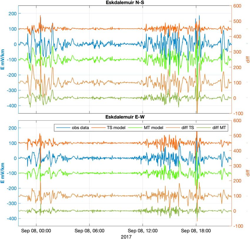
C.D. Beggan et al.: J. Space Weather Space Clim. 2021, 11, 37

in Figure 1c. A similar data collection system to the other obser-
vatories exists. The geoelectric field system in Hartland was
installed in early 2013.
    Data from all three observatories are posted to the BGS
website every 10 min and plots showing the past 6 h, the day
to date and the past 30 days are available for browsing.
Figure 1d shows a stackplot of the north–south component from
Hartland for June 2013. There is a clear lunar tidal signal visible
(approximately 20 mV/km peak to peak) with a period of
12.42 h. Note that some minor space weather activity is visible
at the beginning of Days 1 and 29.
    The geoelectric field systems were installed to test whether
good quality data could be collected at the existing geomagnetic
observatories. Due to the generally challenging environments in
the remote locations and the normal decay of the probes, main-
taining continuous high-quality measurements has not been
possible. Various redesigns of the systems over the years as well
as damage from lightning or component failure have caused
gaps or poor quality data for analysing longer periods. This is
in addition to drifts caused by the degradation of the probes
and occasional steps in the data. However, a considerable effort
has been made to clean up the dataset where feasible and new
instrumentation is planned.
    In addition to the range of geomagnetic latitudes, the three
observatories lie in very different settings in terms of proximity
to the coast, altitude and underlying geology. This gives rise to
strong variations in the electric and magnetic environment
experienced during space weather events. Due to the relatively
quiescent nature of space weather in the approximately eight
years of operation to date, the geoelectric field measurements
encompass relatively few intense events e.g. the 17 March
2015 and the 7–8 September 2017 storms are two of the larger
storms of solar cycle 24.
    Figures 2 and 3 show the minute-mean values of the
magnetic and geoelectric fields recorded at the three observato-
ries for these dates. The upper panels (a–c) shows    the horizontal
                                                  pffiffiffiffiffiffiffiffiffiffiffiffiffiffiffiffi
                                                                  ffi
strength of the magnetic field variation (H ¼ X 2 þ Y 2 ) rela-
tive to its quiet time background (in nT) with the variation of the
two geoelectric horizontal field components (in mV/km). Note
the curves have been offset from each other to show the detail.
It can be observed at each site that it is the high frequency vari-
ations of the magnetic field that induce the geoelectric field with
the long period variations being largely damped. Only Hartland
has long-period variations due to the tidally-induced field from        Fig. 2. Measurements of the geoelectric field components (North–
high range and rapid flow of seawater in the Bristol Channel.           South & East–West), the variation of the horizontal component (H)
    The bottom panel (d) in both figures shows the measured             of the magnetic field and GIC (in amps) for 17–18 March 2015 at: (a)
GIC from a Hall probe installed at Torness 400 kV substation           Lerwick; (b) Eskdalemuir; (c) Hartland; (d) GIC at Torness
in central Scotland, around 90 km northeast of Eskdalemuir             substation, East Scotland. Note the magnetic and geoelectric curves
(McKay, 2003). The GIC response of the high voltage power              are offset from zero.
grid can be considered to be a band-pass filtered version of
the geoelectric field. Again, it is clear that the short-period vari-   various technical issues. Note the variation of the magnetic and
ations of the geoelectric field have the strongest influence on          geoelectric fields are smaller than the 2015 and 2017 storms as
measured GIC.                                                          were the resultant GICs.
    Finally, a storm on the 26 August 2018 is shown in Figure 4.
Though a relatively minor storm (G3 on the NOAA geomag-
netic storm scale), it coincided with the deployment of the
differential magnetometer method (DMM) systems of Hübert               3 Magnetotelluric impedance functions
et al. (2020) which allowed a comparison of both line and
substation GIC to be made. Unfortunately, only a single channel            Using the geoelectric (E) and simultaneous magnetic field
of electric field data at each observatory was in operation due to      (B) measurements at the three observatories we computed the

                                                               Page 4 of 18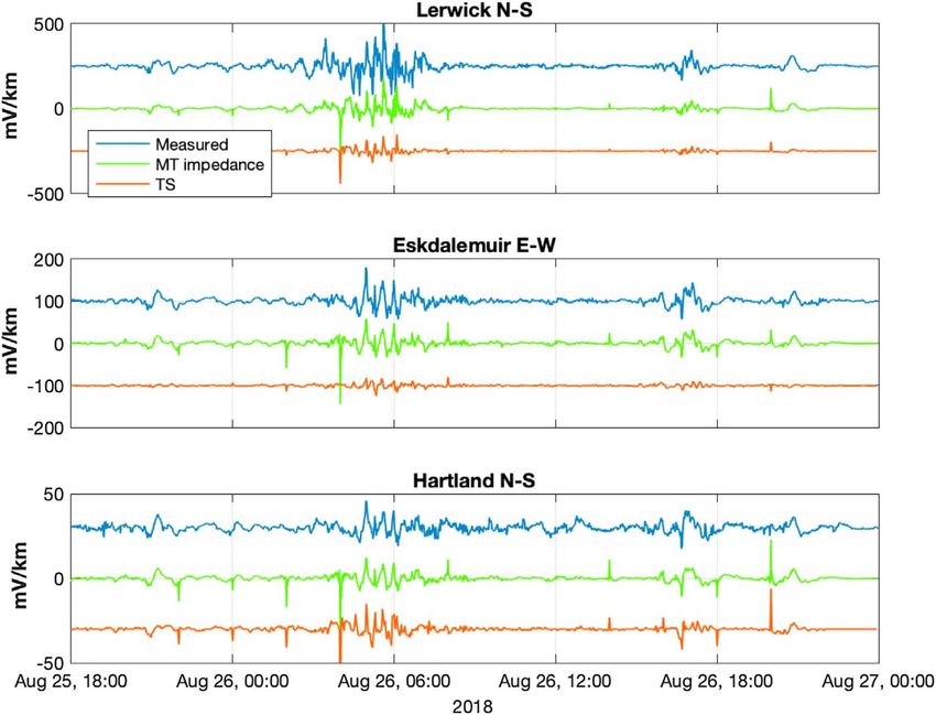
C.D. Beggan et al.: J. Space Weather Space Clim. 2021, 11, 37

Fig. 3. Measurements of the geoelectric field components (North–       Fig. 4. Measurements of the geoelectric field component (North–
South & East–West), the variation of the horizontal component (H)     South or East–West), the variation of the horizontal component (H)
of the magnetic field and GIC (in amps) for 7–8 September 2017. (a)    of the magnetic field and GIC (in amps) for 25–26 August 2018.
Lerwick; (b) Eskdalemuir; (c) Hartland; (d) GIC at Torness            Only one electric channel at each site was available. (a) Lerwick; (b)
substation, East Scotland. Note the magnetic and geoelectric curves   Eskdalemuir; (c) Hartland; (d) GIC from Torness substation, East
are offset from zero.                                                 Scotland. Note the magnetic and geoelectric curves are offset from
                                                                      zero.

magnetotelluric impedance tensor Z at each site (e.g. Wait,
1982). It is defined in the frequency domain as:
                             1                                        the robust statistical algorithm of Smirnov (2008). Z is
                    EðxÞ ¼      ZðxÞ  BðxÞ                    ð1Þ    assumed to be temporarily stationary – it represents the under-
                             l0
                                                                      lying electrical conductivity distribution which can be
with l0 the magnetic permeability and the angular frequency           assumed to be constant in the case of the UK. We tested this
x. We chose six months during 2015 of uninterrupted and rel-          and derived Z from different time periods of recordings at the
atively noise-free time-series from each observatory to derive        three observatories with almost identical outcomes (within the
the impedance in the frequency range of 20–30,000 s using             uncertainties).

                                                              Page 5 of 18
C.D. Beggan et al.: J. Space Weather Space Clim. 2021, 11, 37

Fig. 5. Components of the two-dimensional MT impedance tensor Z at all three UK observatories. Differences in curves reflect the varying
underlying electrical resistivity structure across Britain.

    Figure 5 shows the components of the impedance for                   In the case of dense MT surveys, like in the USA (Schultz
periods of 20–30,000 s for each of the three observatories.          et al., 2006–2018), the interpolation of impedances over the
The transfer functions show the largest response at short periods    whole modelling domain becomes feasible and the estimation
(20–1000 s) with an approximately exponential decrease (i.e. a       of the geoelectric field over larger areas is possible (Bonner &
linear change in logarithmic scale) with longer periods beyond       Schultz, 2017). This is desirable for the accurate modelling of
1000 s. This is consistent with the observations of the geomag-      GICs which requires the integration of electric fields along the
netic to geoelectric response in Figures 2–4. In general, Hartland   affected ground infrastructure like power lines or pipelines
has the weakest magnitude response to magnetic field varia-           which can extend over long distances crossing several regions
tions, while Lerwick and Eskdalemuir have a stronger response.       of lateral conductivity variation. We will use the MT transfer
The differences in the structure of the curves for each compo-       functions to estimate geoelectric fields from historic large storm
nent relate primarily to the geology beneath each site, though       events (see Sect. 5).
at longer periods the associated errors become larger too (not
shown).
    From our observations, during storm times, the geoelectric       4 Thin-sheet modeling of the geoelectric field
field estimates from the MT transfer functions tend to under-
estimate the magnitude of the measured geoelectric field. This            To model the regional geoelectric field, we wish to combine
can be attributed to a number of causes, as discussed for exam-      the response of the ground conductivity in a region with the
ple in Campanya et al. (2019). Some signal loss can be               spatial and temporal measurements of the rate of change of
explained by the limited frequency content (the magnetic field        the horizontal components of the magnetic field. We use a
data is sampled at 1 min and the impedance tensor is only            thin-sheet model to do this which has the advantage that
derived for 10–30,000 s). Additionally, the plane wave approx-       spatially variable magnetic fields can be used as an input. The
imation, fundamental for the MT tensor relationship, may not be      modelling code is based upon the work of Vasseur & Weidelt
able to explain all of the signal during geomagnetic storm times     (1977) which has been employed in previous studies noted in
(Viljanen et al., 1999; Romano et al., 2014; Simpson & Bahr,         the Introduction. The code computes the surface electric field
2020). For example, Simpson & Bahr (2021) demonstrate they           arising at a particular period (for example, 120 s or 2 min) from
require frequency-based correction factors to force their MT         a 2-D conductivity model of the surface and a layered subsur-
transfer functions computed from quiet-time data to match            face. Using a series of Green’s functions convolved with a
storm-time geoelectric field measurements.                            two-dimensional thin-sheet representation of the conductance,

                                                             Page 6 of 18
C.D. Beggan et al.: J. Space Weather Space Clim. 2021, 11, 37
Fig. 6. Left panel: Thin-sheet conductance model of the UK and surrounding seas with a cell size of 10 km (units of log 10 (Siemens)). Right
panel: Block model underlying the thin-sheet conductance model with electrical resistivities assigned according to geologic domains after
Beamish & White (2012).
the effect that conductivity variations have on redistributing three dimensional electrical conductivity distribution in the crust
regional or “normal” currents induced elsewhere (for example, and upper mantle. In the absence of countrywide MT data, it is
in the sea) can be computed. The surface layer can be regarded nevertheless a good first approximation using available data and
as an infinite thin-sheet of finite laterally-variable conductance, geological information.
across which certain boundary conditions apply. The code requires the average rate-of-change of the horizon-
For the top layer, we use conductance values in a 10 km tal magnetic field for a fixed period as an input. Different strate-
grid-cell model of the UK developed by Beamish & White gies can be chosen to incorporate the magnetic field variation
(2012) and Beamish (2013). The lithology-based classification over the area of interest. In previous papers (e.g. Kelly et al.,
of bedrock is used to provide an association with the petrophys- 2017), we have used the DB value of the external field recorded
ical rock parameters controlling bulk conductivity, assumed to every minute at several observatories by assuming the ampli-
represent the conductance to a depth of 3 km. The 10 km tude of the horizontal field changes sinusoidally with a period
map is based on a reduced version of a 1:625 k scale (approx- of length T (in minutes), as an electrojet current system moves
imately 1 km) map, and is comprised of 86 lithological classifi- back and forwards in latitude, the input field strength (H0) at any
cations. Offshore, seawater is assumed to have a conductivity of time (t) can be represented by BH = H0 sin(2pt/T). However,
3 S/m and the model accounts for changes in bathymetry. The this does not impose any bandpass filtering on the input
model extends 1200 1680 km (121 169 cells) and, in order magnetic field and implies a fixed frequency on the output geo-
to reduce edge effects, an additional 5 cells of padding are electric field.
added to each edge to make the final grid of 131 179 cells. Instead, for this study, we adopted an alternative method
The padding cells have values close to of the average suggested in Bailey et al. (2017, 2018) which uses the rate of
conductance of the entire model. Figure 6 (left panel) shows change of the horizontal components of the field (dBX/dt and
the 2D thin-sheet conductance map of the UK. dBY/dt). Their Austrian-based study used the difference in the
Below 3 km, a series of 1D models, each with 20 layers, are magnetic values every 5 min (D t = 300 s) and, in combination
used to represent the underlying structure of the British Isles to a with a model of the country’s high voltage power network,
depth of approximately 1000 km. The shallow to mid-crustal successfully matched the GIC measurements at several sites in
tectonic setup of the the UK can be described by six major geo- the country. We replicate this approach but using a difference
logic terranes. We use the conductivities from the terrane model of 2 min (D t = 120 s) which matches the available magnetic
of Beamish et al. (2002), categorised as the more resistive time-series of minute-mean values. We also refer to Ivannikova
Northern and Central Highlands and the less resistive Midland et al. (2018) who showed that their thin-sheet geoelectric field
Valley and Southern Uplands of Scotland. South of the Iapetus matched that computed with a full 3D model to within 8%
Suture Zone covering much of England lies the Concealed for periods longer than 50 s.
Caledonides terrane with a conductive mid-crustal anomaly To implement this approach, maps of the magnetic field
(Banks et al., 1983). The southern part of the UK is considered across the region are created for each minute of the day using
as part of the Variscan Zone. Ádám et al. (2012) provide values spherical elementary current systems (SECS) to interpolate
for the 1D conductivity models of these terranes. Figure 6 (right between measurement sites (Amm, 1997). The SECS method
panel) shows the resistivity of the models at a depth of 6.5 km. produces good estimates of the magnetic field across the
The influence of these underlying 1D models on the magnitude modelling domain when there are typically greater than five
of the induced geoelectric field at the surface was examined in observatories available in a closely spaced (C.D. Beggan et al.: J. Space Weather Space Clim. 2021, 11, 37
The difference of the magnetic field every 2 min is com-
puted (giving 720 snapshots per day) and each snapshot of
the magnetic field is passed into the thin-sheet code. The output
consists of geoelectric maps for every 2nd min of the day. Note,
we also tested Dt of 5 and 10 min (300 and 600 s) and found
similar patterns of variation, though with smaller amplitude
ranges. In practice, we run the thin-sheet model for each of
the 1D terrane models and combine the results by extracting
the corresponding part of each terrane on land into the final
model. This is, in effect, a blocky pseudo-3D approximation,
similar to Myllys et al. (2014) or Viljanen & Pirjola (2017).
We can then test how well the thin-sheet geoelectric field
values compare to the recorded measurements at the three
observatories. However, there are a number of limitations,
which include the extent of the thin-sheet model and the effect
of regional or local geological features. In the first case, the thin-
sheet model does not extend to the Lerwick Observatory,
though it is quite close to the edge (around 20 km). To extract
the geoelectric field at this site, we must extrapolate the thin-
sheet model slightly, which introduces some additional uncer-
tainty. At Eskdalemuir, it is well known that there is a shallow
local crustal anomaly though this mostly affects the vertical Fig. 7. Location of the INTERMAGNET-standard observatories
magnetic component (Banks et al., 1996). Finally, Hartland is (red), calibrated variometers (green) and variometers (blue) used for
strongly influenced by a tidal geoelectric signal which is not SECS magnetic field interpolation.
captured by the thin-sheet model due to the band-pass filter
applied to produce the dB/dt values; however, we are interested
primarily in the space weather effects which are demonstratively measured and modelled geoelectric field. For the thin-sheet code
shorter-period (see Figs. 2–4). this is related to a convolution and integration of the magnetic
field with the conductivity model over the entire grid.
5.1 March 2015 storm
5 Comparison between electric field models
and measurements The first so-called “super” storm of solar cycle 24 was the
St. Patrick’s Day storm, starting on the 17 March 2015 with
We examine the geoelectric field modelled for three of the the |Dst| index exceeding 200 nT (Wu et al., 2016). The storm
larger storms experienced in the UK between 2013 and 2018: followed a partial-halo Coronal Mass Ejection (CME), associ-
17–18 March 2015, 7–8 September 2017 and 26 August ated with an X-ray solar flare of moderate intensity (C9.1), that
2018. We compare the MT-derived and the thin-sheet model occurred on the surface of the Sun on 15 March 2015. The most
geoelectric field values against the measured data at the three rapid geomagnetic variations were associated with periods of
UK observatories. strongly negative IMF Bz of 20 nT. In the UK, the storm
We isolate the external field part of the magnetic field by exhibited two main bursts of activity on the evening of the 17
removing the average quiet-time mean value of magnetic com- March separated by around 6 h (see Fig. 2).
ponent computed from measurements made a few hours prior to For the March 2015 storm, magnetic data from eight obser-
the storm’s initiation. For example, local night-time values vatories were available, allowing interpolation of the magnetic
between 02:00 and 03:00 LT a day or so prior to a storm are field variation across the UK. The northernmost variometers
often the quietest. The external field will comprise ionospheric are Dombås (DOB) and Karmøy (KAR) in Norway, with
and magnetospheric sources as well as the magnetic effect of Dourbes (DOU) in Belgium being the southernmost observa-
telluric currents which may be a relatively large contribution tory. Wingst (WNG) is the east-most observatory and Valentia
(Juusola et al., 2020). (VAL) is west-most. While not ideal for SECS interpolation, as
To compute the external magnetic field variation over the there is no control in the northwestern region, the spatial distri-
North Sea we used SECS with data from the three BGS obser- bution covers the majority of the thin-sheet modelling area.
vatories complemented with other observatory or variometer The thin-sheet model was run using the north (X) compo-
data from Ireland, the Faroe Islands, France, Germany, nent and east (Y) components of the external magnetic field vari-
Belgium, Denmark and Norway in order to expand the region ation for a response period of 120 s. In order to compare to the
over which the external magnetic field can be computed. modelled field, the measured geoelectric field data were band-
Figure 7 shows the spatial extent of the magnetic measurements passed between 120 and 3600 s using a Butterworth 3-pole
available. Note not all stations are available for each storm (see filter. As the geoelectric field data are recorded at 10 Hz, this
Table 1). In general, we find using a larger number of magnetic removes much of the very short-period and some of the long
observatories creates a better model of the magnetic field over period energy though as we noted in the previous section longer
the region, which in turn produces a better match between the period variations do not have much influence on GIC.
Page 8 of 18C.D. Beggan et al.: J. Space Weather Space Clim. 2021, 11, 37
Table 1. Stations with magnetic data available for SECS interpolation.
Storm Stations
Mar 2015 DOB, DOU, ESK, HAD, KAR, LER, VAL, WNG
Sep 2017 ARM, BIR, BGS3, BGS7, BGS9, BGS10, CRK, DOB, DOU, ESK
HAD, HOV, KAR, LAN, LER, SID, SOL, SUM, VAL, WNG
Aug 2018 BGS10, CRK, DOU, ESK, HAD, HOV, LER, SOL, VAL, WNG
Mar 1989 CRK, ESK, HAD, LER, VAL, WNG
Oct 2003 CRK, DOB, DOU, ESK, HAD, FAR, KAR, LER, VAL, WNG
Figure 8 shows the comparison of the geoelectric field mea- the northwestern area of the model. In total, magnetic data from
surements made at each observatory for the March 2015 storm. twenty sites were collected, giving an excellent representation of
The measured data in blue, the MT-derived values are in green the magnetic field variation across Britain and Ireland. As
and the thin-sheet modelled values are in red. In Lerwick the before, data were processed to remove the quiet time mean
geoelectric field variation reached over 1 V/km peak-to-peak value of the horizontal components at each site, using the value
around 18:00 UT in the east component, while it was around for 02:00–03:00 local time from 7 September. Where the
50% smaller at Eskdalemuir with a peak-to-peak change of orientation of the sensor is unknown (as with the Raspberry
500 mV/km. At the most southerly observatory, Hartland, the Pi magnetometers) we rotated the quiet time horizontal compo-
geoelectric field in this frequency band reaches around nents to match the estimated values of X and Y from a global
50 mv/km peak-to-peak. magnetic field model, the 12th generation of the International
For the east component of the thin-sheet electric field at Geomagnetic Reference Field (Thébault et al., 2015). The
Lerwick the magnitude is not well captured, though the match thin-sheet model was run for the storm using two days’ worth
is better in the north component. The MT values are of magnetic values for both the X and the Y magnetic field
closer, though do not match the peak values at all times. At components.
Eskdalemuir, the thin-sheet comparison in phase and amplitude Figure 9 shows the resulting band-pass filtered thin-sheet
is much better in the north component compared to the east model output compared to the band-passed measurements of
component, while in Hartland the magnitude is similar though the geoelectric field from each observatory. The intensity of the
the correlation is poorer (see Sect. 5.4 for further detail). As September storm is comparable to, if not larger than, the March
the east–west geoelectric field component of the thin-sheet 2015 storm in terms of the peak-to-peak variations at each obser-
model is poorest at the two northerly sites, it suggests a problem vatory. The plots show the two large substorms around midnight
with modelling the variation of the magnetic field in these areas of the 7th September and 12:00–18:00 on the 8th. The electric
due to the limited spatial extent of ground stations used. field variation is over 1 V/km in Lerwick, 500 mV/km in
Eskdalemuir and 80 mV/km in Hartland. Note that the large
5.2 September 2017 storm values in Hartland around 21:00 on the 8th are an artefact.
For this storm, the thin-sheet model has performed better in
On 7 September 2017 one of the largest storms of the capturing the magnitude and phase of the geoelectric field at all
24th solar cycle hit the Earth (Dimmock et al., 2019). A three sites. The MT values provide a good estimate of the geo-
CME left the Sun at midday on 6 September and reached electric field too, matching best at Eskdalemuir and Hartland.
Earth’s magnetosphere around 36 h later. Starting about We provide a more comprehensive quantitative evaluation of
23:30 UT on 7 September, the first and deepest part of the storm the data fit see Section 5.4.
lasted for around 3 h, reaching a Dst of 124 nT. At 13:00 UT
on 8 September a second substorm was triggered, though not as 5.3 August 2018 storm
large as the first part of the storm (Fig. 3).
To get a regional picture of the storm, data were collected Although the August 2018 storm was a relatively small
from a network of Raspberry Pi magnetometers (denoted event in the solar cycle, it was the largest storm of the year with
BGS3/7/9/10) (Beggan & Marple, 2018), as well as a number a peak Kp of 7+. The total interplanetary magnetic field reached
of other variometers and observatories around the UK, Ireland, a strength of 21 nT with a prolonged period of southward Bz and
Belgium, Germany and Norway including the observatories the Dst index had a peak of 174 nT. The storm was likely
(from INTERMAGNET), the Lancaster University Aurora- caused by a CME though no classic shock signature was
Watch network of variometers (Case et al., 2017), a network observed. The storm coincided with the deployment of differen-
in Ireland run by Trinity College Dublin (MagIE) (Blake tial magnetometer method (DMM) system which allowed a
et al., 2016) and data from the Tromsø Geophysical Observa- detailed analysis of GICs in the 400 kV high voltage power grid
tory (TGO) network. The SOL and KAR sites host calibrated in East Scotland (Hübert et al., 2020).
variometers which provide the variation of the field in addition For the magnetic field interpolation, fewer variometers
the absolute values of the geomagnetic field vector, though the were available for this storm (only 10 stations, e.g. due to main-
data are not as well controlled as at full observatories (where tenance issues), so the SECS model of the field is not as accurate
weekly baseline measurements are conducted). We also as for the September 2017 storm. Magnetic data are available
received data from the DTU-operated Faroe Islands Hov from Hov in the Faroe Islands in the north to Dourbes in
variometer, which helped to constrain the field variations in Belgium to the south and we include some of the AuroraWatch
Page 9 of 18C.D. Beggan et al.: J. Space Weather Space Clim. 2021, 11, 37
(a)
(b)
(c)
(d)
(e)
(f)
Fig. 8. Comparison of the thin-sheet (TS), magnetotelluric (MT impedance) and measured geoelectric field at (a, b) Lerwick, (c, d)
Eskdalemuir and (e, f) Hartland observatories for 17 March 2015.
and BGS school magnetometer data. In addition, as noted in examined. Lerwick has a peak-to-peak variation of around
Section 2, the geoelectric field probes at LER, ESK and HAD 250 mV/km in the north component, while Eskdalemuir reaches
only have data from one channel available at each site, due to around 100 mV/km in the east component. The geoelectric field
a mixture of equipment failure and probe degradation. in Hartland is very small, barely exceeding 20 mV/km peak-to-
Figure 10 shows the measured, MT-derived and thin-sheet peak. Similar to March 2015, the north component of Lerwick
modelled geoelectric field values. The overall magnitude of is poorly captured by the thin-sheet model in the main phase.
the field is much smaller than during the other two storms The E–W geoelectric field component at Eskdalemuir is better
Page 10 of 18C.D. Beggan et al.: J. Space Weather Space Clim. 2021, 11, 37
(a)
(b)
(c)
(d)
(e)
(f)
Fig. 9. Comparison of the thin-sheet (TS), magnetotelluric (MT impedance) and measured geoelectric field at (a, b) Lerwick, (c, d)
Eskdalemuir and (e, f) Hartland observatories for 7–8 September 2017.
modelled, though not as well as the September 2017 storm, cannot be captured by the regional model. This means that
while Hartland has very small geoelectric field values and so direct correlations between the time-series can be low despite
the comparison is difficult to judge. appearing close.
To account for this we use a selection of metrics to assess
5.4 Metrics to assess data fit between measured quantitatively how well the models match the measurements.
and modelled electric field data As well as the standard correlation between the time-series,
following Torta et al. (2014), we compute the P-metric for each
When comparing relatively “noisy” data sets such as the storm using,
geoelectric field values, it is difficult to provide an over-arching
metric that best describes the match between the model and RMSDom
P ¼1 ð2Þ
measurements as minor fluctuations in the local geoelectric field ro
Page 11 of 18C.D. Beggan et al.: J. Space Weather Space Clim. 2021, 11, 37
(a)
(b)
(c)
Fig. 10. Comparison of the thin-sheet (TS), magnetotelluric (MT impedance) and measured geoelectric field at (a) Lerwick, (b) Eskdalemuir
and (c) Hartland observatories for 26 August 2018. Note only one channel was available at each site.
Table 2. Metric comparisons for three storms with thin-sheet-derived geoelectric field values.
Storm Metric LER (N–S) LER (E–W) ESK (N–S) ESK (E–W) HAD (N–S) HAD (E–W)
Mar-15 RMSDom 114.4 41.8 19.3 39.5 6.4 6.5
P 0.09 0.01 0.17 0.06 0.29 0.24
Correlation 0.68 0.24 0.58 0.33 0.01 0.07
Sep-17 RMSDom 45.6 96.0 18.9 19.8 5.0 6.0
P 0.18 0.01 0.25 0.24 0.13 0.02
Correlation 0.58 0.32 0.59 0.66 0.44 0.46
Aug-18 RMSDom 18.0 – – 6.4 2.2 –
P 0.15 – – 0.08 0.05 –
Correlation 0.54 – – 0.47 0.25 –
where ro is the standard deviation of the set of observations transmission grid and found that rarely did P exceed 0.4, even
and RMSDom is the root mean square deviation of the resid- with visually close match between their time-series.
uals (i.e. differences between model predictions and Table 2 gives a series of metrics for the correlation of
observations), the measured data and thin-sheet time-series shown in
vffiffiffiffiffiffiffiffiffiffiffiffiffiffiffiffiffiffiffiffiffiffiffiffiffiffiffi Figures 8–10. For the March 2015 storm, the correlation is
uN
uP surprisingly high for the north–south component of Lerwick
u ðoi mi Þ2
t and Eskdalemuir at 0.68 and 0.58, but is around zero for
RMSDom ¼ i¼1 : ð3Þ Hartland. The P values for Lerwick and Eskdalemuir are very
N
small though (0.09 and 0.17).
The September 2017 storm shows again that the
The values oi and mi are the ith point (of N samples) of the correlation can be high though the P metric is negative. For
observation and model. The maximum value of P cannot Eskdalemuir in the N–S component, there is a good
exceed 1 where the model exactly fits the observations. How- match between the time-series but it has a P value of 0.25
ever, if P is zero or less there is little direct predictive power, with a correlation of 0.59. Finally, the thin-sheet electric
though a negative value of P does not necessarily imply an field estimates for the August 2018 storm are moderately corre-
anti-correlation. Torta et al. (2014) examined time-series of lated for Lerwick (0.54) and Eskdalemuir (0.47) but low for
GIC measurements versus GIC models in the Spanish power Hartland (0.25).
Page 12 of 18C.D. Beggan et al.: J. Space Weather Space Clim. 2021, 11, 37
Table 3. Metric comparisons for three storms with the impedance-derived geoelectric field values.
Storm Metric LER (N–S) LER (E–W) ESK (N–S) ESK (E–W) HAD (N–S) HAD (E–W)
Mar-15 RMSDom 27.58 50.67 11.21 8.2 1.75 2.0
P 0.24 0.36 0.56 0.42 0.50 0.39
Correlation 0.79 0.89 0.95 0.90 0.94 0.92
Sep-17 RMSDom 25.5 33.6 8.3 4.7 2.3 1.89
P 0.15 0.6 0.48 0.53 0.16 0.38
Correlation 0.91 0.92 0.97 0.95 0.88 0.94
Aug-18 RMSDom 16.1 – – 5.5 2.4 –
P 0.03 – – 0.24 0.28 –
Correlation 0.76 – – 0.76 0.52 –
Fig. 11. The measured geoelectric field (blue, offset from zero) and differences between it and the thin-sheet (red) and magnetotelluric (green)
models at ESK for the 7–8 September 2017.
For the MT-derived geoelectric field time-series, the correla- tables illustrate this point – that the correlation between the
tions with the measured values are given in Table 3. Again, the models can be good but the P metric is often not high and
correlations with each observatory are very high (generally occasionally close to zero. a direct comparison of the models
0.75–0.95), as expected, as the impedance functions are derived and measurements is shown in Figure 11. The differences
from the measurements at each site. However, the P values are between the measured values of the geoelectric field and those
quite mixed from 0.24 at Lerwick for the March 2015 storm modelled by thin-sheet and MT method for the 7/8th September
to 0.56 for Eskdalemuir during the same storm. Hence, even if 2017 at Eskdalemuir are plotted. The north–south direction of
the correlation is high, the time-series can also have a low the thin-sheet model has a negative P value (0.25) even
P value when there is a large difference in the magnitude. though the correlation is quite high (0.59) (see Fig. 9). In
The differences between the measurements and models can contrast, the east–west component has P value of 0.24 with a
be large and occasionally similar in magnitude. The metric correlation of 0.66. This is an example where the phase of the
Page 13 of 18C.D. Beggan et al.: J. Space Weather Space Clim. 2021, 11, 37
Fig. 12. Upper (a, b): Predicted geoelectric fields for the March 1989 storm. Lower (c, d): Predicted geoelectric fields for the October 2003
storm.
geoelectric field variation is well captured by both models, but east–west component. The geoelectric field at Hartland
the magnitude is not. does not exceed 0.16 V/km. The thin-sheet model shows
similar magnitude peaks though generally around 30% lower
(e.g. 0.7 V/km compared to 1 V/km in Lerwick north
6 Historic storms component).
For the October 2003 storm, the estimated geoelectric
Using the MT impedance functions for each site, the one- fields overall are slightly smaller. Eskdalemuir experienced
minute-mean magnetic field measurements from the 13–14 larger values in the north–south component compared to
March 1989 to 29–31 October 2003 were used to estimate the Lerwick late on the 30th October with one large period of
geoelectric field (Campanya et al., 2019; Hübert et al., 2020). almost 3 V/km. The larger magnetic (and hence geoelectric)
The main limitation of this approach is the plane-wave assump- fields experienced at Eskdalemuir in the north–south component
tion of the magnetic field for the MT response functions, which may be related to rapid expansion of the auroral oval during
is generally applicable only for geomagnetically quiet times at storm times (Freeman et al., 2019). The geoelectric field values
mid to low latitudes. for Hartland are generally small for both storms and indeed not
Figure 12 shows the geoelectric field values for both storms much larger than those measured during the September 2017
computed from the MT impedance and the thin-sheet modelling storm for example.
code. For the thin-sheet model, fewer observatory data were
available compared to the analyses in Section 4 (see Table 1)
so the magnetic field is not as well captured across the region. 7 Discussion
For the MT-derived values, the March 1989 storm has electric
field amplitudes of up to 1 V/km at Lerwick in the north–south Measurements of the magnetic and geoelectric field at the
component, around midnight on 13 March, and 2.3 V/km in the three UK observatories illustrate that the Earth acts as a high-
east–west component. The north–south component at pass filter during geomagnetic storms, removing much of the
Eskdalemuir shows a maximum value of 1.7 V/km around this long magnetic field period variation beyond 1 h. Between
time as well, though the fields are smaller (0.75 V/km) in the 2012 and 2020, the maximum absolute value of the
Page 14 of 18C.D. Beggan et al.: J. Space Weather Space Clim. 2021, 11, 37
geoelectric field recorded was around 1 V/km at the Lerwick the modelling of geoelectric fields across the UK for space
observatory, while at Eskdalemuir 0.5 V/km was measured. weather purposes in a similar manner to Marshall et al.
Only at Hartland is the geoelectric field visibly dominated by (2019) and Lucas et al. (2020).
a long-period tidal signal generated by seawater flow in the
Bristol Channel.
By combining the geoelectric and magnetic field measure- 8 Conclusions
ments at the observatories, MT impedance tensors can be
computed which provide estimates of geoelectric fields during The geoelectric field is a key driver of geomagnetically
the large geomagnetic storms, for example, those of March induced currents in grounded infrastructure. Successfully
1989 and October 2003. The MT-derived geoelectric values modelling this field is essential for providing real-time estimates
have a maximum of around 3 V/km at Eskdalemuir for the of hazard to the high voltage power network. Due to the diverse
October 2003 storm. However, GIC measurements at the time geological and topographical structure of the UK, the geoelec-
suggest the geoelectric field was likely to have been even larger. tric field varies in a complex manner, both spatially and
Thomson et al. (2005) show GIC data measured at Torness sub- temporally.
station which imply the geoelectric field was between 3 and 4 We describe the three main strands of research to understand
V/km at the peak of the 2003 storm as currents of 20 A were and model the geoelectric field in the UK during severe space
recorded (at a one-second cadence). Recent work on validation weather events. Firstly, continuous measurements of the geo-
of the high voltage network model at Torness in Hübert et al. electric field at a cadence of 10 Hz have been on-going at the
(2020) corroborates well with this analysis. Given the limited three UK observatories since 2012. Although several major
number of large storms in the period of 2012–2020 when geo- storms have been observed between 2012 and 2020, none have
electric field data are available to create the impedance func- been large enough to cause known issues with technical infras-
tions, the estimates shown here should be considered as a tructure. The largest absolute magnitude of the geoelectric field
lower bound of the geoelectric field generated during extreme measured was around 1 V/km at Lerwick in March 2015.
space weather events. We also note that only minute-mean data Magnetotelluric impedance functions are computed from the
of historic magnetic field data are available, which reduces the geoelectric field and magnetic measurements at the three obser-
peak magnitude modelled during these storms because the vatories allowing an estimate to be made of the geoelectric field
energy content of the higher frequencies is not included. during past storms such as the March 1989 and October 2003
The comparison of the modelled geoelectric fields from the storms. However, we find that MT transfer functions computed
thin-sheet model with the measured data shows an imperfect from quiet time tend to underestimate the magnitude of the geo-
match. This is not unexpected, given the limitations of the mod- electric field during storm times.
elling technique and the input assumptions regarding the under- Modelling using the thin-sheet methodology allows us to
lying geology as a contribution to the electrical conductivity compute near-real-time estimates of the field though at the cost
model and variation of the magnetic data across the region. of reduced accuracy. From comparison with geoelectric mea-
The advantages of using the thin-sheet model, however, include surements at three observatories, we conclude the thin-sheet
the ability to use snapshot maps of the magnetic field variation model provides some predictive power, though this is typically
both spatially and temporally and the reasonably quick compu- an underestimate of the true value of the geoelectric field.
tation time. Providing the spatial variation of the geoelectric Future work will involve updating the geoelectric probes at
field is necessary for modelling GICs in the grounded infrastruc- each observatory as the original hardware reaches the end-of-
ture. The quick computation time also allows the thin-sheet life, installing new variometers in the UK and to continue to
model to be used as a real-time now-cast system and as a fore- collect magnetotelluric data from sites around Britain to aid
casting tool, assuming suitable estimates of the magnetic field the modelling of geoelectric fields for real-time and forecasting
are available. Increasing the number of variometers in the region applications.
supplying real-time data would also be very useful in improving
the geoelectric field estimate. Acknowledgements. We wish to acknowledge the Geomag-
Finally, the metrics in Section 5.4 illustrate the problems of netism engineering team (Chris Turbitt, Simon Flower, Tom
the various approximations within the thin-sheet model. In Martyn, Tony Swan, Tom Shanahan and Tim Taylor) for
general, the larger the magnitude of the geoelectric field, the bet- installing and maintaining the geoelectric field probes at the
ter the model matches. It is also worth noting that September three BGS observatories. Geoelectric field data were pro-
2017 is best modelled because of the denser spatial coverage cessed as part of an MSc. by Research at the University of
of observatory and variometer data to create a good representa- Edinburgh by O. Baillie. The results presented in this paper
tion of the magnetic field. It is also of note that the MT-derived rely on data collected at magnetic observatories. We thank
field values have a generally high correlation but a wide range the national institutes that support them and INTERMAGNET
of P values which indicates that P is sensitive to small levels of for promoting high standards of magnetic observatory practice
noise or magnitude differences between time-series. (https://www.intermagnet.org). We also thank the providers of
On-going and future work within the UK NERC-funded variometer data in Ireland, Faroe Islands, Norway and the UK.
SWIGS and SWIMMR projects will provide an island-wide Real-time geoelectric field data are available at http://www.
MT survey, at a resolution of around 70 km, similar to the geomag.bgs.ac.uk/data_service/space_weather/geoelectric.html.
EarthScope project in the USA. We also plan to install new This work is funded under UK Natural Environment Research
variometers at three further sites in the UK to improve spatial Council Grant NE/P017231/1 “Space Weather Impact on
coverage. From these new datasets, we will be able improve Ground-based Systems (SWIGS)”. This work has also received
Page 15 of 18You can also read