Functional and Effective Connectivity: A Review - Translational ...
←
→
Page content transcription
If your browser does not render page correctly, please read the page content below
BRAIN CONNECTIVITY
Volume 1, Number 1, 2011
ª Mary Ann Liebert, Inc.
DOI: 10.1089/brain.2011.0008
Functional and Effective Connectivity: A Review
Karl J. Friston
Abstract
Over the past 20 years, neuroimaging has become a predominant technique in systems neuroscience. One might
envisage that over the next 20 years the neuroimaging of distributed processing and connectivity will play a major
role in disclosing the brain’s functional architecture and operational principles. The inception of this journal has
been foreshadowed by an ever-increasing number of publications on functional connectivity, causal modeling,
Downloaded by Eth Bibliothek from www.liebertpub.com at 08/15/20. For personal use only.
connectomics, and multivariate analyses of distributed patterns of brain responses. I accepted the invitation to
write this review with great pleasure and hope to celebrate and critique the achievements to date, while address-
ing the challenges ahead.
Key words: causal modeling; brain connectivity; effective connectivity; functional connectivity
Introduction application of these advances in the setting of hierarchical
brain architectures.
T his review of functional and effective connectivity in
imaging neuroscience tries to reflect the increasing inter-
est and pace of development in this field. When discussing
The Fundaments of Connectivity
Here, we will establish the key dichotomies, or axes, that
the nature of this piece with Brain Connectivity’s editors, I
frame the analysis of brain connectivity in both a practical
got the impression that Dr. Biswal anticipated a scholarly re-
and a conceptual sense. The first distinction we consider is be-
view of the fundamental issues of connectivity in brain imag-
tween functional segregation and integration. This distinction
ing. On the other hand, Dr. Pawela wanted something
has a deep history, which has guided much of brain mapping
slightly more controversial and engaging, in the sense that
over the past two decades. A great deal of brain mapping is
it would incite discussion among its readers. I reassured
concerned with functional segregation and the localization
Chris that if I wrote candidly about the background and cur-
of function. However, last year the annual increase in publi-
rent issues in connectivity research, there would be more than
cations on connectivity surpassed the yearly increase in pub-
sufficient controversy to keep him happy. I have therefore ap-
lications on activations per se (see Fig. 1). This may reflect a
plied myself earnestly to writing a polemic and self-referen-
shift in emphasis from functional segregation to integration:
tial commentary on the development and practice of
the analysis of distributed and connected processing appeals
connectivity analyses in neuroimaging.
to the notion of functional integration among segregated
This review comprises three sections. The first represents
brain areas and rests on the key distinction between func-
a brief history of functional integration in the brain, with a
tional and effective connectivity. We will see that this distinc-
special focus on the distinction between functional and ef-
tion not only has procedural and statistical implications for
fective connectivity. The second section addresses more
data analysis but also is partly responsible for a segregation
pragmatic issues. It pursues the difference between func-
of the imaging neuroscience community interested in these is-
tional and effective connectivity, and tries to clarify the re-
sues. The material in this section borrows from its original for-
lationships among various analytic approaches in light of
mulation in Friston et al. (1993) and an early synthesis in
their characterization. In the third section, we look at recent
Friston (1995).
advances in the modeling of both experimental and endog-
enous network activity. To illustrate the power of these ap-
Functional segregation and integration
proaches thematically, this section focuses on processing
hierarchies and the necessary distinction between forward From a historical perspective, the distinction between func-
and backward connections. This section concludes by con- tional segregation and functional integration relates to the
sidering recent advances in network discovery and the dialectic between localizationism and connectionism that
The Wellcome Trust Centre for Neuroimaging, University College London, London, United Kingdom.
13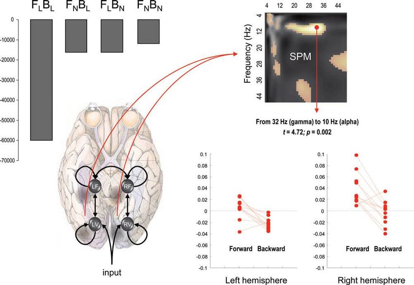
14                                                                                                                           FRISTON

                                                                                           FIG. 1. Publication rates pertaining to functional segregation and integration. Publications per year searching for ‘‘Activa-
                                                                                           tion’’ or ‘‘Connectivity’’ and functional imaging. This reflects the proportion of studies looking at functional segregation (ac-
                                                                                           tivation) and those looking at integration (connectivity). Source: PubMed.gov. U.S. National Library of Medicine. The image
Downloaded by Eth Bibliothek from www.liebertpub.com at 08/15/20. For personal use only.

                                                                                           on the left is from the front cover of The American Phrenological Journal: Vol. 10, No. 3 (March) 1846.

                                                                                           dominated ideas about brain function in the 19th century.            dromes and the refutation of localizationism as a complete
                                                                                           Since the formulation of phrenology by Gall, the identifica-         or sufficient account of cortical organization. Functional local-
                                                                                           tion of a particular brain region with a specific function has       ization implies that a function can be localized in a cortical
                                                                                           become a central theme in neuroscience. Somewhat ironically,         area, whereas segregation suggests that a cortical area is spe-
                                                                                           the notion that distinct brain functions could be localized was      cialized for some aspects of perceptual or motor processing,
                                                                                           strengthened by early attempts to refute phrenology. In 1808,        and that this specialization is anatomically segregated within
                                                                                           a scientific committee of the Athénée at Paris, chaired by Cuv-    the cortex. The cortical infrastructure supporting a single
                                                                                           ier, declared that phrenology was unscientific and invalid           function may then involve many specialized areas whose
                                                                                           (Staum, 1995). This conclusion may have been influenced              union is mediated by the functional integration among
                                                                                           by Napoleon Bonaparte (after an unflattering examination             them. In this view, functional segregation is only meaningful
                                                                                           of his skull by Gall). During the following decades, lesion          in the context of functional integration and vice versa.
                                                                                           and electrical stimulation paradigms were developed to test
                                                                                           whether functions could indeed be localized in animals. The
                                                                                                                                                                Functional and effective connectivity
                                                                                           initial findings of experiments by Flourens on pigeons were
                                                                                           incompatible with phrenologist predictions, but later experi-           Imaging neuroscience has firmly established functional
                                                                                           ments, including stimulation experiments in dogs and mon-            segregation as a principle of brain organization in humans.
                                                                                           keys by Fritsch, Hitzig, and Ferrier, supported the idea that        The integration of segregated areas has proven more difficult
                                                                                           there was a relation between distinct brain regions and spe-         to assess. One approach to characterize integration is in terms
                                                                                           cific functions. Further, clinicians like Broca and Wernicke         of functional connectivity, which is usually inferred on the
                                                                                           showed that patients with focal brain lesions showed specific        basis of correlations among measurements of neuronal activ-
                                                                                           impairments. However, it was realized early on that it was           ity. Functional connectivity is defined as statistical dependen-
                                                                                           difficult to attribute a specific function to a cortical area,       cies among remote neurophysiological events. However,
                                                                                           given the dependence of cerebral activity on the anatomical          correlations can arise in a variety of ways. For example, in mul-
                                                                                           connections between distant brain regions. For example, a            tiunit electrode recordings, correlations can result from stimu-
                                                                                           meeting that took place on August 4, 1881, addressed the dif-        lus-locked transients evoked by a common input or reflect
                                                                                           ficulties of attributing function to a cortical area given the de-   stimulus-induced oscillations mediated by synaptic connec-
                                                                                           pendence of cerebral activity on underlying connections              tions (Gerstein and Perkel, 1969). Integration within a distrib-
                                                                                           (Phillips et al., 1984). This meeting was entitled Localization      uted system is usually better understood in terms of effective
                                                                                           of Function in the Cortex Cerebri. Goltz (1881), although            connectivity: effective connectivity refers explicitly to the influ-
                                                                                           accepting the results of electrical stimulation in dog and mon-      ence that one neural system exerts over another, either at a syn-
                                                                                           key cortex, considered the excitation method inconclusive, in        aptic or population level. Aertsen and Preißl (1991) proposed
                                                                                           that the movements elicited might have originated in related         that ‘‘effective connectivity should be understood as the exper-
                                                                                           pathways or current could have spread to distant centers. In         iment and time-dependent, simplest possible circuit diagram
                                                                                           short, the excitation method could not be used to infer func-        that would replicate the observed timing relationships be-
                                                                                           tional localization because localizationism discounted inter-        tween the recorded neurons.’’ This speaks to two important
                                                                                           actions or functional integration among different brain              points: effective connectivity is dynamic (activity-dependent),
                                                                                           areas. It was proposed that lesion studies could supplement          and depends on a model of interactions or coupling.
                                                                                           excitation experiments. Ironically, it was observations on pa-          The operational distinction between functional and effec-
                                                                                           tients with brain lesions several years later (see Absher and        tive connectivity is important because it determines the na-
                                                                                           Benson, 1993) that led to the concept of disconnection syn-          ture of the inferences made about functional integration and
FUNCTIONAL AND EFFECTIVE CONNECTIVITY 15
the sorts of questions that can be addressed. Although this spaces to find a model or network (graph) that has the great-
distinction has played an important role in imaging neurosci- est evidence. Because model evidence is a function of both the
ence, its origins lie in single-unit electrophysiology (Gerstein model and data, analysis of effective connectivity is both
and Perkel, 1969). It emerged as an attempt to disambiguate model (hypothesis) and data led. The key aspect of effective
the effects of a (shared) stimulus-evoked response from those connectivity analysis is that it ultimately rests on model com-
induced by neuronal connections between two units. In neuro- parison or optimization. This contrasts with analysis of func-
imaging, the confounding effects of stimulus-evoked responses tional connectivity, which is essentially descriptive in nature.
are replaced by the more general problem of common inputs Functional connectivity analyses usually entail finding the
from other brain areas that are manifest as functional connectiv- predominant pattern of correlations (e.g., with principal or in-
ity. In contrast, effective connectivity mediates the influence dependent component analysis [ICA]) or establishing that a
that one neuronal system exerts on another and, therefore, dis- particular correlation between two areas is significant. This
counts other influences. We will return to this below. is usually where such analyses end. However, there is an im-
portant application of functional connectivity that is becom-
Coupling and connectivity ing increasingly evident in the literature. This is the use of
functional connectivity as an endophenotype to predict or
Put succinctly, functional connectivity is an observable
classify the group from which a particular subject was sam-
phenomenon that can be quantified with measures of statisti-
pled (e.g., Craddock et al., 2009).
cal dependencies, such as correlations, coherence, or transfer
Indeed, when talking to people about their enthusiasm for
entropy. Conversely, effective connectivity corresponds to
resting-state (design-free) analyses of functional connectivity,
the parameter of a model that tries to explain observed de-
Downloaded by Eth Bibliothek from www.liebertpub.com at 08/15/20. For personal use only.
this predictive application is one that excites them. The ap-
pendencies (functional connectivity). In this sense, effective
peal of resting-state paradigms is obvious in this context:
connectivity corresponds to the intuitive notion of coupling
there are no performance confounds when studying patients
or directed causal influence. It rests explicitly on a model
who may have functional deficits. In this sense, functional
of that influence. This is crucial because it means that the anal-
connectivity has a distinct role from effective connectivity.
ysis of effective connectivity can be reduced to model
Functional connectivity is being used as a (second-order)
comparison—for example, the comparison of a model with
data feature to classify subjects or predict some experimental
and without a particular connection to infer its presence. In
factor. It is important to realize, however, that the resulting
this sense, the analysis of effective connectivity recapitulates
classification does not test any hypothesis about differences
the scientific process because each model corresponds to an
in brain coupling. The reason for this is subtle but simple:
alternative hypothesis about how observed data were caused.
in classification problems, one is trying to establish a map-
In our context, these hypotheses pertain to causal models of
ping from imaging data (physiological consequences) to a di-
distributed brain responses. We will see below that the role
agnostic class (categorical cause). This means that the model
of model comparison becomes central when considering differ-
comparison pertains to a mapping from consequences to
ent modeling strategies. The philosophy of causal modeling and
causes and not a generative model mapping from causes to
effective connectivity should be contrasted with the procedures
consequences (through hidden neurophysiological states).
used to characterize functional connectivity. By definition, func-
Only analyses of effective connectivity compare (generative)
tional connectivity does not rest on any model of statistical de-
models of coupling among hidden brain states.
pendencies among observed responses. This is because
In short, one can associate the generative models of effec-
functional connectivity is essentially an information theoretic
tive connectivity with hypotheses about how the brain
measure that is a function of, and only of, probability distribu-
works, while analyses of functional connectivity address the
tions over observed multivariate responses. This means that
more pragmatic issue of how to classify or distinguish sub-
there is no inference about the coupling between two brain re-
jects given some measurement of distributed brain activity.
gions in functional connectivity analyses: the only model com-
In the latter setting, functional connectivity simply serves as
parison is between statistical dependency and the null model
a useful summary of distributed activity, usually reduced to
(hypothesis) of no dependency. This is usually assessed with
covariances or correlations among different brain regions.
correlation coefficients (or coherence in the frequency domain).
In a later section, we will return to this issue and consider
This may sound odd to those who have been looking for differ-
how differences in functional connectivity can arise and
ences in functional connectivity between different experimental
how they relate to differences in effective connectivity.
conditions or cohorts. However, as we will see later, this may
It is interesting to reflect on the possibility that these two
not be the best way of looking for differences in coupling.
distinct agendas (generative modeling and classification)
are manifest in the connectivity community. Those people in-
Generative or predictive modeling?
terested in functional brain architectures and effective con-
It is worth noting that functional and effective connectivity nectivity have been meeting at the Brain Connectivity
can be used in very different ways: Effective connectivity is Workshop series every year (www.hirnforschung.net/bcw/).
generally used to test hypotheses concerning coupling archi- This community pursues techniques like dynamic causal
tectures that have been probed experimentally. Different modeling (DCM) and Granger causality, and focuses on
models of effective connectivity are compared in terms of basic neuroscience. Conversely, recent advances in functional
their (statistical) evidence, given empirical data. This is connectivity studies appear to be more focused on clinical
just evidence-based scientific hypothesis testing. We will and translational applications (e.g., ‘‘with a specific focus
see later that this does not necessarily imply a purely on psychiatric and neurological diseases’’; www.canlab
hypothesis-led approach to effective connectivity; network .de/restingstate/). It will be interesting to see how these
discovery can be cast in terms of searches over large model two communities engage with each other in the future,
16 FRISTON
especially as the agendas of both become broader and less that are mediated by changes in cognitive set or unfold over
distinct. This may be particularly important for a mechanis- time due to synaptic plasticity. These sorts of effects have mo-
tic understanding of disconnection syndromes and other tivated the development of nonlinear models of effective con-
disturbances of distributed processing. Further, there is a nectivity that consider explicitly interactions among synaptic
growing appreciation that classification models (mapping inputs (e.g., Friston et al., 1995; Stephan et al., 2008). In short,
from consequences to causes) may be usefully constrained connectivity is as transient, adaptive, and context-sensitive as
by generative models (mapping from causes to conse- brain activity per se. Therefore, it is unlikely that characteriza-
quences). For example, generative models can be used to tions of connectivity that ignore this will furnish deep insights
construct an interpretable and sparse feature-space for sub- into distributed processing. So what is the role of structural
sequent classification. This ‘‘generative embedding’’ was in- connectivity?
troduced by Brodersen and associates (2011a), who used Structural constraints on the generative models used for ef-
dynamic causal models of local field potential recordings fective connectivity analysis are paramount when specifying
for single-trial decoding of cognitive states. This approach plausible models. Further (in principle) they enable more pre-
may be particularly attractive for clinical applications, cise parameter estimates and more efficient model compari-
such as classification of disease mechanisms in individual son. Having said this, there is remarkably little evidence
patients (Brodersen et al., 2011b). Before turning to the tech- that quantitative structural information about connections
nical and pragmatic implications of functional and effective helps with inferences about effective connectivity. There
connectivity, we consider structural or anatomical connec- may be several reasons for this. First, effective connectivity
tivity that has been referred to, appealingly, as the connec- does not have to be mediated by monosynaptic connections.
Downloaded by Eth Bibliothek from www.liebertpub.com at 08/15/20. For personal use only.
tome (Sporns et al., 2005). Second, quantitative information about structural connec-
tions may not predict their efficacy. For example, the influ-
ence or effective connectivity of the (sparse and slender)
Connectivity and the connectome
ascending neuromodulatory projections from areas like the
In the many reviews and summaries of the definitions used ventral tegmental area may far exceed the influence predicted
in brain connectivity research (e.g., Guye et al., 2008; Sporns, by their anatomical prevalence. The only formal work so far
2007), researchers have often supplemented functional and that demonstrates the utility of tractography estimates is
effective connectivity with structural connectivity. In recent reported in Stephan et al. (2009). This work compared dy-
years, the fundamental importance of large-scale anatomical namic causal models of effective connectivity (in a visual in-
infrastructures that support effective connections for cou- terhemispheric integration task) that were and were not
pling has reemerged in the context of the connectome and at- informed by structural priors based on tractography. The au-
tendant graph theoretical treatments (Bassett and Bullmore, thors found that models with tractography priors had more
2009; Bullmore and Sporns, 2009; Sporns et al., 2005). This evidence than those without them (see Fig. 2 for details).
may, in part, reflect the availability of probabilistic tractogra- This provides definitive evidence that structural constraints
phy measures of extrinsic (between area) connections from on effective connectivity furnish better models. Crucially,
diffusion tensor imaging (Behrens and Johansen-Berg, the tractography priors were not on the strength of the con-
2005). The status of structural connectivity and its relation- nections, but on the precision or uncertainty about their
ship to functional effective connectivity is interesting. I see strength. In other words, structural connectivity was shown
structural connectivity as furnishing constraints or prior be- to play a permissive role as a prior belief about effective con-
liefs about effective connectivity. In other words, effective nectivity. This is important because it means that the exis-
connectivity depends on structural connectivity, but struc- tence of a structural connection means (operationally) that
tural connectivity per se is neither a sufficient nor a complete the underlying coupling may or may not be expressed.
description of connectivity. A potentially exciting development in diffusion tensor im-
I have heard it said that if we had complete access to the con- aging is the ability to invert generative models of axonal
nectome, we would understand how the brain works. I suspect structure to recover much more detailed information about
that most people would not concur with this; it presupposes the nature of the underlying connections (Alexander, 2008).
that brain connectivity possesses some invariant property A nice example here is that if we were able to estimate the di-
that can be captured anatomically. However, this is not the ameter of extrinsic axonal connections between two areas
case. Synaptic connections in the brain are in a state of constant (Zhang and Alexander, 2010), this might provide useful pri-
flux showing exquisite context-sensitivity and time- or activity- ors on their conduction velocity (or delays). Conduction de-
dependent effects (e.g., Saneyoshi et al., 2010). These are man- lays are a free parameter of generative models for
ifest over a vast range of timescales, from synaptic depression electrophysiological responses (see below). This raises the
over a few milliseconds (Abbott et al., 1997) to the maintenance possibility of establishing structure–function relationships in
of long-term potentiation over weeks. In particular, there are connectivity research, at the microscopic level, using nonin-
many biophysical mechanisms that underlie fast, nonlinear vasive techniques. This is an exciting prospect that several
‘‘gating’’ of synaptic inputs, such as voltage-dependent ion of my colleagues are currently pursuing.
channels and phosphorylation of glutamatergic receptors by
dopamine (Wolf et al., 2003). Even structural connectivity
Summary
changes over time, at microscopic (e.g., the cycling of postsyn-
aptic receptors between the cytosol and postsynaptic mem- This section has introduced the distinction between func-
brane) and macroscopic (e.g., neurodevelopmental) scales. tional segregation and integration in the brain and how the
Indeed, most analyses of effective connectivity focus specifi- differences between functional and effective connectivity
cally on context- or condition-specific changes in connectivity shape the way we characterize connections and the sorts of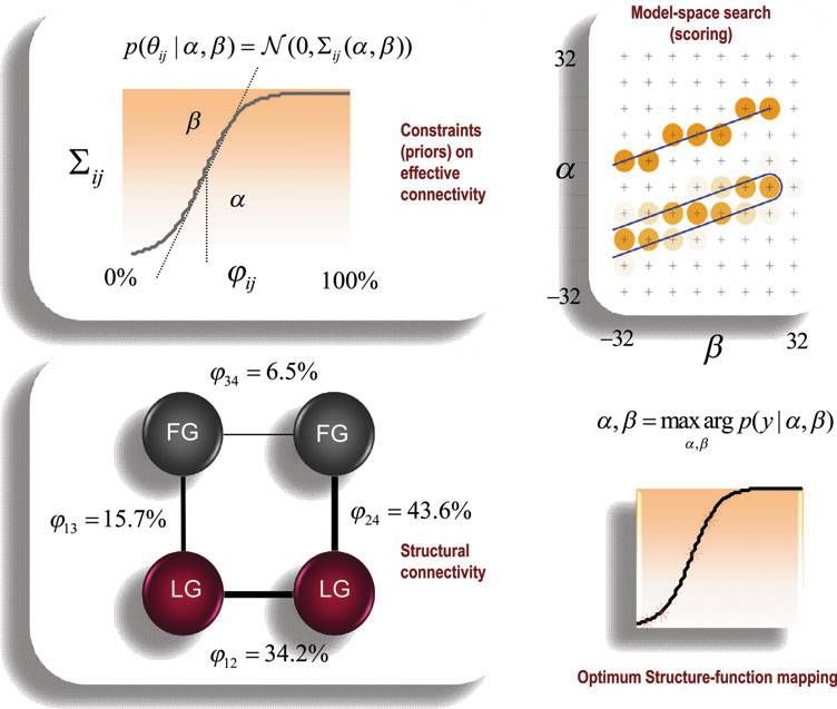
FUNCTIONAL AND EFFECTIVE CONNECTIVITY 17
FIG. 2. Structural con-
straints on functional connec-
tions. This schematic
illustrates the procedure
reported in Stephan et al.
(2009), providing evidence
that anatomical tractography
measures provide informa-
tive constraints on models
and effective connectivity.
Consider the problem of esti-
mating the effective connec-
tivity among some regions,
given quantitative (if proba-
bilistic) estimates of their an-
atomical connection strengths
(demoted by uij). This is il-
lustrated in the lower left
panel using bilateral areas in
the lingual and fusiform gyri.
The first step would be to
Downloaded by Eth Bibliothek from www.liebertpub.com at 08/15/20. For personal use only.
specify some mapping be-
tween the anatomical infor-
mation and prior beliefs
about the effective connec-
tions. This mapping is illus-
trated in the upper left panel,
by expressing the prior vari-
ance on effective connectivity
(model parameters h) as a
sigmoid function of anatomi-
cal connectivity, with un-
known hyperparameters a b m, where m denotes a model. We can now optimize the model in terms of its hyperparameters
and select the model with the highest evidence p(yjm), as illustrated by model scoring on the upper right. When this was done
using empirical data, tractography priors were found to have a sensible and quantitatively important role. The inset on the
lower right shows the optimum relationship between tractography estimates and prior variance constraints on effective
connectivity. The four asterisks correspond to the four tractography measures shown on the lower left [see Stephan et al. (2009)
for further detail].
questions that are addressed. We have touched upon the role discussion of how to compare connectivity between conditions
of structural connectivity in providing constraints on the ex- or groups. The material here is a bit technical but uses a tutorial
pression of effective connectivity or coupling among neuro- style that tries to suppress unnecessary mathematical details
nal systems. In the next section, we look at the relationship (with a slight loss of rigor and generality).
between functional and effective connectivity and how the
former depends upon the latter. A generative model of coupled neuronal systems
We start with a generic description of distributed neuronal
Analyzing Connectivity and other physiological dynamics, in terms of differential
equations. These equations describe the motion or flow,
This section looks more formally at functional and effective
f(x, u, h), of hidden neuronal and physiological states, x(t),
connectivity, starting with a generic (state-space) model of the
such as synaptic activity and blood volume. These states
neuronal systems that we are trying to characterize. This nec-
are hidden because they are not observed directly. This
essarily entails a generative model and, implicitly, frames the
means we also have to specify mapping, g(x, u, h), from
problem in terms of effective connectivity. We will look at
hidden states to observed responses, y(t):
ways of identifying the parameters of these models and com-
paring different models statistically. In particular, we will con- x_ ¼ f (x, u, h) þ x
sider successive approximations that lead to simpler models (1)
y ¼ g(x, u, h) þ v
and procedures commonly employed to analyze connectivity.
In doing this, we will hopefully see the relationships among the Here, u(t) corresponds to exogenous inputs that might en-
different analyses and the assumptions on which they rest. To code changes in experimental conditions or the context under
make this section as clear as possible, it will use a toy example which the responses were observed. Random fluctuations
to quantify the implications of various assumptions. This ex- x(t) and v(t) on the motion of hidden states and observa-
ample uses a plausible connectivity architecture and shows tions render Equation (1) a random or stochastic differential
how changes in coupling, under different experimental condi- equation. One might wonder why we need both exogenous
tions or cohorts, would be manifest as changes in effective or (deterministic) and endogenous (random) inputs; whereas
functional connectivity. This section concludes with a heuristic the exogenous inputs are generally known and under experi-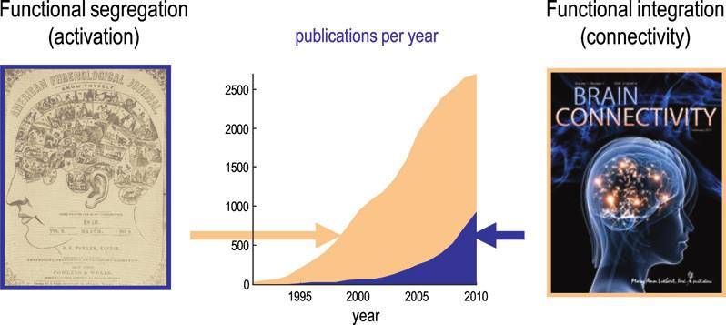
18 FRISTON
mental control, endogenous inputs represent unknown influ- Here, superscripts indicate whether the parameters refer to
ences (e.g., from areas not in the model or spontaneous fluctu- the strength of connections, hx, their context-dependent (bilin-
ations). These can only be modeled probabilistically (usually ear) modulation, hxu, or the effects of perturbations or exoge-
under Gaussian, and possibly Markovian, assumptions). nous inputs, hu. To keep things very simple, we will further
Clearly, the equations of motion (first equality) and observer pretend that we have direct access to hidden neuronal states
function (second equality) are, in reality, immensely compli- and that they are measured directly (as in invasive electro-
cated equations of very large numbers of hidden states. In physiology). This means we can ignore hemodynamics and
practice, there are various theorems such as the center mani- the observer function (for now). Equation (3) parameterizes
fold theorem* and slaving principle, which means one can re- connectivity in terms of partial derivatives of the state-
duce the effective number of hidden states substantially but equation. For example, the network in Figure 3 can be de-
still retain the underlying dynamical structure of the system scribed with the following effective connectivity parameters:
(Ginzburg and Landau, 1950; Carr, 1981; Haken, 1983; Kopell 2 3 2 3 2 3
:5 0:2 0 0 0:2 0 0
and Ermentrout, 1986). The parameters of these equations, h, 6 7 6 7 6 7
include effective connectivity and control how hidden states hx ¼ 4 0:3 :3 0 5 hxu ¼ 4 0 0 0 5 hu ¼ 4 0 5 (4)
in one part of the brain affect the motion of hidden states else- 0:6 0 :4 0 0 0 0
where. Equation (1) can be regarded as a generative model of
observed data that is specified completely, given assumptions Here, the input u 2 f0, 1g encodes a condition or cohort-spe-
about the random fluctuations and prior beliefs about the cific effect that selectively increases the (backward) coupling
states and parameters. Inverting or fitting this generative from the second to the first node or region (from now on
we will use effective connectivity and coupling synonymous-
Downloaded by Eth Bibliothek from www.liebertpub.com at 08/15/20. For personal use only.
model corresponds to estimating its unknown states and pa-
rameters (effective connectivity), given some observed data. ly). These values have been chosen as fairly typical for fMRI.
This is called dynamic causal modeling (DCM) and usually Note that the exogenous inputs do not exert a direct (activat-
employs Bayesian techniques. ing) effect on hidden states, but act to increase a particular
However, the real power of DCM lies in the ability to com- connection and endow it with context-sensitivity. Note fur-
pare different models of the same data. This comparison rests ther that we have assumed that hidden neuronal dynamics
on the model evidence, which is simply the probability of the can be captured with a single state for each area. We will
observed data, under the model in question (and known ex- now consider the different ways in which one can try to esti-
ogenous inputs). The evidence is also called the marginal like- mate these parameters.
lihood because one marginalizes or removes dependencies on
the unknown quantities (states and parameters). Dynamic causal modeling
Z As noted above, DCM would first select the best model
p(yjm, u) ¼ p(y, x, hjm, u)dxdh (2) using Bayesian model comparison. Usually, different models
are specified in terms of priors on the coupling parameters.
Model comparison rests on the relative evidence for one These are used to switch off parameters by assuming a priori
model compared to another [see Penny et al. (2004) for a that they are zero (to create a new model). For example, if we
discussion in the context of functional magnetic resonance wanted to test for the presence of a backward connection
imaging (fMRI). Likelihood-ratio tests of this sort are com-
monplace. Indeed, one can cast the t-statistic as a likelihood
ratio. Model comparison based on the likelihood of different
models will be a central theme in this review and provides the
quantitative basis for all evidence-based hypothesis testing.
In this section, we will see that all analyses of effective con-
nectivity can be reduced to model comparison. This means
the crucial differences among these analyses rest with the
models on which they are based.
Clearly, to search over all possible models (to find the one
with the most evidence) is generally impossible. One, there-
fore, appeals to simplified but plausible models. To illustrate
this simplification and to create an illustrative toy example,
we will use a local (bilinear) approximation to Equation (1)
of the sort used in DCM of fMRI time series (Friston et al.,
2003) and with a single exogenous input, u 2 f0, 1g:
x_ ¼ hx x þ uhxu x þ hu u þ x
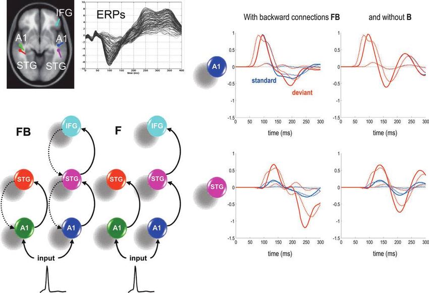
FIG. 3. Toy connectivity architecture. This schematic shows
x vf xu v2 f vf (3) the connections among three brain areas or nodes that will be
h ¼ h ¼ hu ¼
vx vxvu vu x ¼ 0, u ¼ 0 used to demonstrate the relationship between effective con-
nectivity and functional connectivity in the main text. To
highlight the role of changes in connectivity, the right graph
shows the connection that changes (over experimental condi-
tion or diagnostic cohort) as the thick black line. This is an ex-
*Strictly speaking, the center manifold theorem is used to reduce ample of a directed cyclic graph. It is cyclic by virtue of the
the degrees of freedom only in the neighborhood of a bifurcation. reciprocal connections between A1 and A2.
FUNCTIONAL AND EFFECTIVE CONNECTIVITY 19
from the second to the first area, hx12 , we would compare two The second equality expresses this vector autoregression
models with the following priors: model as a simple general linear model with explanatory var-
x, that correspond to a time-lagged (time · region) ma-
iables, ~
p(hx12 jm0 ) ¼ N (0, 0)
(5) trix of states and unknown parameters in the autoregression
p(hx12 jm1 ) ¼ N (0, 8) matrix, A = exp(Dhx). Note that the random fluctuations or in-
novations, e(t), are now a mixture of past fluctuations in x(t)
These Gaussian (shrinkage) priors force the effective con-
that are remembered by the system.
nectivity to be zero under the null model m0 and allow it to
We now have a new model whose parameters are autore-
take large values under m1. Given sufficient data, the Bayes-
gression coefficients that can be tested using classical likeli-
ian model comparison would confirm that the evidence for
hood ratio tests. In other words, we can compare the
the alternative model was greater than the null model,
likelihood of models with and without a particular regression
using the logarithm of the evidence ratio:
coefficient, Aij, using classical model comparison based on the
p(yjm1 ) extra sum of squares principle (e.g., the F-statistic). For n
ln ¼ ln p(yjm1 ) ln p(yjm0 )
p(yjm0 ) (6) states and e*N (0, r2 I), these tests are based on the sum of
F(y, l1 ) F(y, l0 ) squares and products of the residuals, Ri : i = 0,1, under the
maximum likelihood solutions of the alternative and null
Notice that we have expressed the logarithm of the mar- models, respectively:
ginal likelihood ratio as a difference in log-evidences. This
is a preferred form because model comparison is not limited p(yjm1 )
to two models, but can cover a large number of models whose ln ln p(yjl1 , m1 ) ln p(yjl0 , m0 )
Downloaded by Eth Bibliothek from www.liebertpub.com at 08/15/20. For personal use only.
p(yjm0 ) (8)
quality can be usefully quantified in terms of their log-evi- n n
dences. (We will see an example of this in the last section.) ¼ 2 ln jR1 j 2 ln jR0 j
2r 2r
A relative log-evidence of three corresponds to a marginal
likelihood ratio (Bayes factor) of about 20 to 1, which is usu- This is Granger causality (Granger, 1969) and has been
ally considered strong evidence in favor of one model over used in the context of autoregressive models of fMRI data
another (Kass and Raftery, 1995). An important aspect of (Roebroeck et al., 2005, 2009). Note that Equation (8) uses
model evidence is that it includes a complexity cost (which likelihoods as opposed to marginal likelihoods to approxi-
is not only sensitive to the number of parameters but mate the evidence. This (ubiquitous) form of model compar-
also to their interdependence). This means that a model ison assumes that the posterior density over unknown
with redundant parameters would have less evidence, even quantities can be approximated by a point mass over the
though it provided a better fit to the data (see Penny et al., conditional mean. In the absence of priors, this is their
2004). maximum likelihood value. In other words, we ignore
In most current implementations of DCM, the log-evidence uncertainty about the parameters when estimating the evi-
is approximated with a (variational) free-energy bound that dence for different models. This is a reasonable heuristic
(by construction) is always less than the log-evidence. This but fails to account for differences in model complexity
bound is a function of the data and (under Gaussian assump- (which means the approximation in Equation (8) is never
tions about the posterior density) some proposed values for less than zero).
the states and parameters. When the free-energy is maxi- The likelihood model used in tests of Granger causality as-
mized (using gradient ascent) with respect to the proposed sumes that the random terms in the vector autoregression
values, they become the maximum posterior or conditional model are (serially) independent. This is slightly problematic
estimates, l, and the free-energy, F(y, l)p ln p(yjm), ap- given that these terms acquire temporal correlations when
proaches the log-evidence. We will return to the Bayesian converting the continuous time formulation into the discrete
model comparison and inversion of dynamic causal models time formulation [see Equation (7)]. The independence (Mar-
in the next section. At the moment, we will consider some kovian) assumption means that the network has forgotten
alternative models. The first is a discrete-time linear approx- past fluctuations by the time it is next sampled (i.e., it is not
imation to Equation 1, which is the basis of Granger causality. sampled very quickly). However, there is a more fundamen-
tal problem with Granger causality that rests on the fact that
the autoregression parameters of Equation (7) are not the cou-
Vector autoregression models and Granger causality pling parameters of Equation (3). In our toy example, with a
One can convert any dynamic causal model into a linear repetition time of D = 2.4 seconds, the true autoregression co-
state-space or vector autoregression model (Goebel et al., efficients are
2003; Harrison et al., 2003; see Rogers et al., 2010 for review) 2 3
by solving (integrating) the Taylor approximation to Equa- :5 0:2 0
6 7
tion (3) over the intervals between data samples, D, using hx ¼ 4 0:3 :3 0 50 A ¼ exp (2:4 hx )
the matrix exponential. For a single experimental context 0:6 0 :4
(the first input level, u = 0), this gives: 2 3 (9)
:365 :196 0
xt ¼ Axt D þ et 0x ¼ ~xAT þ e 6 7
¼ 4 :295 :561 0 5
A ¼ exp (Dhx ) :521 :137 :383
ZD (7)
et ¼ exp (shx )x(t s)ds This means, with sufficient data, area A2 Granger causes
0 A3 (with a regression coefficient of 0.137) and that any likeli-20 FRISTON
hood ratio test for models with and without this connection Marinazzo et al., 2010) brings it one step closer to DCM (at
will indicate its existence. The reason for this is that we least from my point of view). As noted above, autoregression
have implicitly reparameterized the model in terms of regres- models assume the innovations are temporally uncorrelated.
sion coefficients and have destroyed the original parameteri- In other words, random fluctuations are fast, in relation to
zation in terms of effective connectivity. Put simply, this neuronal dynamics. We will now make the opposite assump-
means the model comparison is making inferences about sta- tion, which leads to the models that underlie structural equa-
tistical dependencies over time as modeled with an autore- tion modeling.
gressive process, not about the causal coupling per se. In
this sense, Granger causality could be regarded as a measure Structural equation modeling
of lagged functional connectivity, as opposed to effective con-
If we now use an adiabatic approximation{ and assume
nectivity. Interestingly, the divergence between Granger cau-
that neuronal dynamics are very fast in relation to random
sality and true coupling increases with the sampling interval.
fluctuations, we can simplify the model above by removing
This is a particularly acute issue for fMRI given its long rep-
the dynamics. In other words, we can assume that neuronal
etition times (TR).
activity has reached steady-state by the time we observe it.
There are many other interesting debates about the use of
The key advantage of this is that we can reduce the generative
Granger causality in fMRI time series analysis [see Valdés-
model so that it predicts, not the time series, but the observed
Sosa et al. (2011) for a full discussion of these issues]. Many
covariances among regional responses over time, Sy.
relate to the effects of hemodynamic convolution, which is ig-
For simplicity, we will assume that g(x, y, h) = x and u = 0. If
nored in most applications of Granger causality (see Chang
the rate of change of hidden states is zero, Eqs. (1) and (3)
Downloaded by Eth Bibliothek from www.liebertpub.com at 08/15/20. For personal use only.
et al., 2008; David et al., 2008). A list of the assumptions
mean that
entailed by the use of a linear autoregression model for
fMRI includes hx x ¼ x0y ¼ v (hx ) 1 x
The hemodynamic response function is identical in all re- 0
T (10)
gions studied. Sy ¼ Sv þ (hx ) 1 Sx (hx ) 1
The hemodynamic response is measured with no noise.
Sy ¼ ÆyyT æ Sv ¼ ÆvvT æ Sx ¼ ÆxxT æ
Neuronal dynamics are linear with no changes in cou-
pling. Expressing the covariances in terms of the coupling param-
Neuronal innovations (fluctuations) are stationary. eters enables one to compare structural equation models
Neuronal innovations (fluctuations) are Markovian. using likelihoods based on the observed sample covariances.
The sampling interval (TR) is smaller than the time con-
stants of neuronal dynamics. p(yjm1 )
ln ln p(Sy jl1 , m1 ) ln p(Sy jl0 , m0 ) (11)
The sampling interval (TR) is greater than the time con- p(yjm0 )
stants of the innovations. The requisite maximum likelihood estimates of the cou-
pling and covariance parameters, l, can now be estimated
It is clear that these assumptions are violated in fMRI and in a relatively straightforward manner, using standard co-
that Granger causality calls for some scrutiny. Indeed, a re- variance component estimation techniques. Note that we do
cent study (Smith et al., 2010) used simulated fMRI time series not have to estimate hidden states because the generative
to compare Granger causality against a series of procedures model explains observed covariances in terms of random
based on functional connectivity (partial correlations, mutual fluctuations and unknown coupling parameters [see Equa-
information, coherence, generalized synchrony, and Bayesian tion (10)]. The form of Equation (10) has been derived from
networks; e.g., Baccalá and Sameshima, 2001; Marrelec et al., the generic generative model. In this form, it can be regarded
2006; Patel et al., 2006). They found that Granger causality as a Gaussian process model, where the coupling parameters
(and its frequency domain variants, such as directed partial become, effectively, parameters of the covariance among ob-
coherence and directed transfer functions; e.g., Geweke, served signals due to hidden states. Although we have de-
1984) performed poorly and noted that rived this model from differential equations, structural
equation modeling is usually described as a regression anal-
The spurious causality estimation that is still seen in the ysis. We can recover the implicit regression model in Equa-
absence of hemodynamic response function variability most tion (10) by separating the intrinsic or self-connections
likely relates to the various problems described in the Granger (which we will assume to be modeled by the identity matrix)
literature (Nalatore et al., 2007; Nolte et al., 2008; Tiao and Wei, and the off-diagonal terms. This gives an instantaneous re-
1976; Wei, 1978; Weiss, 1984); it is known that measurement gression model, hx = h I 0 x = hx + x, whose maximum
noise can reverse the estimation of causality direction, and likelihood parameters can be estimated in the usual way
the temporal smoothing means that correlated time series (under appropriate constraints).
are estimated to [Granger] ‘‘cause’’ each other. So, is this a useful way to characterize effective connectiv-
ity in an imaging time series? The answer to this question de-
It should be noted that the deeper mathematical theory of pends on the adiabatic assumption that converts the dynamic
Granger causality (due to Wiener, Akaike, Granger, and model into a static model. Effectively, one assumes that ran-
Schweder) transcends its application to a particular model
(e.g., the linear autoregression model above). Having said
this, each clever refinement and generalization of Granger {
In other words, we assume that neural dynamics are an adiabatic
causality (e.g., Deshpande et al., 2010; Havlicek et al., 2010; process that adapts quickly to slowly fluctuating perturbations.FUNCTIONAL AND EFFECTIVE CONNECTIVITY 21
dom fluctuations change very slowly in relation to underly- in Equation (12). The Fourier transforms of these kernels
ing physiology, such that it has time to reach steady state. (transfer functions) can be used to compute the coherence
Clearly, this is not appropriate for electrophysiological and among regions at any particular frequency. In our toy exam-
fMRI time series, where the characteristic time constants of ple, the functional connections for the two experimental con-
neuronal dynamics (tens of milliseconds) and hemodynamics texts are (for equal covariance among random fluctuations
(seconds) are generally much larger than the fluctuating or and observation noise, Sx = Sv = 1):
exogenous inputs that drive them. This is especially true 2 3 2 3
1 :407 :414 1 :777 :784
when eliciting neuronal responses using event-related de-
Cu ¼ 0 ¼ 4 :407 1 :410 5 Cu ¼ 1 ¼ 4 :777 1 :769 5
signs. Having said this, structural equation modeling may
:414 :410 1 :784 :769 1
have a useful role in characterizing nontime-series data,
such as the gray matter segments analyzed in voxel-based (13)
morphometry or images of cerebral metabolism acquired There are two key observations here. First, although there
with positron emission tomography. Indeed, it was in this is no coupling between the second and third area, they show
setting that structural equation modeling was introduced to a profound functional connectivity as evidenced by the corre-
neuroimaging: The first application of structural equation lations between them in both contexts (0.41 and 0.769, respec-
modeling used 2-deoxyglucose images of the rat auditory tively). This is an important point that illustrates the problem
system (McIntosh and Gonzalez-Lima, 1991), followed by a of common input (from the first area) that the original distinc-
series of applications to positron emission tomography data tion between functional and effective connectivity tried to ad-
(McIntosh et al., 1994; see also Protzner and McIntosh, 2006). dress (Gerstein and Perkel, 1969). Second, despite the fact that
Downloaded by Eth Bibliothek from www.liebertpub.com at 08/15/20. For personal use only.
There is a further problem with using structural equation the only difference between the two networks lies in one
modeling in the analysis of effective connectivity: it is difficult (backward) connection (from the second to the first area),
to estimate reciprocal and cyclic connections efficiently. Intui- this single change has produced large and distributed
tively, this is because fitting the sample covariance means that changes in functional connectivity throughout the network.
we have thrown away a lot of information in the original time We will return to this issue below when commenting on the
series. Heuristically, the ensuing loss of degrees of freedom comparison of connection strengths. First, we consider briefly
means that conditional dependencies among the estimates the different ways in which distributed correlations can be
of effective connectivity are less easy to resolve. This means characterized.
that, typically, one restricts analyse to simple networks that
are nearly acyclic (or, in the special case of path analysis, Correlations, components, and modes
fully acyclic), with a limited number of loops that can be iden-
tified with a high degree of statistical precision. In machine From the perspective of generative modeling, correlations
learning, structural equation modeling can be regarded as a are data features that summarize statistical dependencies
generalization of inference on linear Gaussian Bayesian net- among brain regions. As such, one would not consider
works that relaxes the acyclic constraint. As such, it is a gen- model comparison because the correlations are attributes of
eralization of structural causal modeling, which deals with the data, not the model. In this sense, functional connectivity
directed acyclic graphics. This generalization is important in can be regarded as descriptive. In general, the simplest way to
the neurosciences because of the ubiquitous reciprocal con- summarize a pattern of correlations is to report their eigen-
nections in the brain that render its connectivity cyclic or re- vectors or principal components. Indeed, this is how voxel-
cursive. We will return to this point when we consider wise functional connectivity was introduced (Friston et al.,
structural causal modeling in the next section. 1993). Eigenvectors correspond to spatial patterns or modes
that capture, in a step down fashion, the largest amount of ob-
Functional connectivity and correlations served covariance. Principal component analysis is also
known as the Karhunen-Loève transform, proper orthogonal
So far, we have considered procedures for identifying ef- decomposition, or the Hotelling transform. The principal
fective connectivity. So, what is the relationship between components of our simple example (for the first context) are
functional connectivity and effective connectivity? Almost the following columns:
universally in fMRI, functional connectivity is assessed with 2 3
the correlation coefficient. These correlations are related :577 :518 :631
mathematically to effective connectivity in the following eig(Cu ¼ 0 ) ¼ 4 :575 :807 :136 5 (14)
way (for simplicity, we will again assume that g(x, y, h) = x :579 :284 :764
and u = 0): When applying the same analysis to resting-state correla-
1 1
C ¼ diag(Sy ) 2 Sy diag(Sy ) 2 tions, these columns would correspond to the weights that
Z1 define intrinsic brain networks (Van Dijk et al., 2010). In
(12) general, the weights of a mode can be positive and nega-
Sy ¼ Sv þ exp (shx )Sx exp (shx )T ds
tive, indicating those regions that go up and down together
0
over time. In Karhunen-Loève transforms of electrophysio-
These equations show that correlation is based on the co- logical time series, this presents no problem because posi-
variances over regions, where these covariances are induced tive and negative changes in voltage are treated on an
by observation noise and random fluctuations. Crucially, be- equal footing. However, in fMRI research, there appears
cause the system has memory, we have to consider the his- to have emerged a rather quirky separation of the positive
tory of the fluctuations causing observed correlations. The and negative parts of a spatial mode (e.g., Fox et al., 2009)
effect of past fluctuations is mediated by the kernels, exp(shx), that are anticorrelated (i.e., have a negative correlation).22 FRISTON
This may reflect the fact that the physiological interpreta- that there has been some change in the distributed activity ob-
tion of activation and deactivation is not completely sym- served in one context and another and that this change is man-
metrical in fMRI. Another explanation may be related to ifest in the correlation [see Equation (13)]. Clearly, this is not a
the fact that spatial modes are often identified using spatial problem if one is only interested in using correlations to predict
independent component analysis (ICA). the cohort or condition from which data were sampled. How-
ever, it is important not to interpret a difference in correlation
Independent component analysis. ICA has very similar as a change in coupling. The correlation coefficient reports
objectives to principal component analysis (PCA), but as- the evidence for a statistical dependency between two areas,
sumes the modes are driven by non-Gaussian random fluctu- but changes in this dependency can arise without changes in
ations (Calhoun and Adali, 2006; Kiviniemi et al., 2003; coupling. This is particularly important for Granger causality,
McKeown et al., 1998). If we reprieve the assumptions of where it might be tempting to compare Granger causality, ei-
structural equation modeling [Equation (10)], we can regard ther between two experimental situations or between directed
principal component analysis as based up the following gen- connections between two nodes. In short, a difference in evi-
erative model: dence (correlation, coherence, or Granger causality) should
not be taken as evidence for a difference in coupling. One can
x ¼ Wx
illustrate this important point with three examples of how a
W ¼ (hx ) 1 (15) change in correlation could be observed in the absence of a
x ~ N(0, Sx ) change in effective connectivity.
By simply replacing Gaussian assumptions about random
Downloaded by Eth Bibliothek from www.liebertpub.com at 08/15/20. For personal use only.
Changes in another connection. Because functional con-
fluctuations with non-Gaussian (supra-Gaussian) assump- nectivity can be expressed at a distance from changes in effec-
tions, we can obtain the generative model on which ICA is tive connectivity, any observed change in the correlation
based. The aim of ICA is to identify the maximum likelihood between two areas can be easily caused by a coupling change
estimates of the mixing matrix, W = (hx)1, given observed co- elsewhere. Using our example above, we can see immediately
variances. These correspond to the modes above. However, that the correlation between A1 and A2 changes when we in-
when performing ICA over voxels in fMRI, there is one final crease the backward connection strength from A2 to A1.
twist. For computational reasons, it is easier to analyze sample Quantitatively, this is evident from Equation (13), where:
correlations over voxels than to analyze the enormous (voxel · 2 3
voxel) matrix of correlations over time. Analyzing the smaller 0 :369 :370
(time · time) matrix is known as spatial ICA (McKeown et al., 4
DC ¼ Cu ¼ 1 Cu ¼ 0 ¼ :369 0 :359 5 (16)
1998). [See Friston (1998) for an early discussion of the relative :370 :359 0
merits of spatial and temporal ICA.] In the present context, this
means that the modes are independent (and orthogonal) over This is perfectly sensible and reflects the fact that statistical
space and that the temporal expression of these independent dependencies among the nodes of a network are exquisitely
components may be correlated. Put plainly, this means that in- sensitive to changes in coupling anywhere. So, does this
dependent components obtained by spatial ICA may or may mean a change in a correlation can be used to infer a change
not be functionally connected in time. I make this point be- in coupling somewhere in the system? No, because the corre-
cause those from outside the fMRI community may be con- lation can change without any change in coupling.
fused by the assertion that two spatial modes (intrinsic brain
networks) are anticorrelated. This is because they might as- Changes in the level of observation noise. An important
sume temporal ICA (or PCA) was used to identify the fallacy of comparing correlation coefficients rests on the fact
modes, which are (by definition) uncorrelated. that correlations depend on the level of observation noise.
This means that one can see a change in correlation by simply
changing the signal-to-noise ratio of the data. This can be par-
Changes in connectivity ticularly important when comparing correlations between
So far, we have focused on comparing different models or different groups of subjects. For example, obsessive compul-
network architectures that best explain observed data. We sive patients may have a heart rate variability that differs
now look more closely at inferring quantitative changes in cou- from normal subjects. This may change the noise in observed
pling due to experimental manipulations. As noted above, there hemodynamic responses, even in the absence of neuronal dif-
is a profound difference between comparing effective connec- ferences or changes in effective connectivity. We can simulate
tion strengths and functional connectivity. In effective connec- this effect, using Equation (12) above, where, using noise lev-
tivity modeling, one usually makes inferences about coupling els of Sv = 1 and Sv = 1.252, we obtain the following difference
changes by comparing models with and without an effect of ex- in correlations:
perimental context or cohort. These effects correspond to the bi- 2 3
0 :061 :060
linear parameters hxu in Equation (3). If model comparison
DC ¼ 4 :061 0 :048 5 (17)
supported the evidence for the model with a context or cohort :060 :048 0
effect, one would then conclude the associated connection (or
connections) had changed. However, when comparing func- These changes are just due to increasing the standard devi-
tional connectivity, one cannot make any comment about ation of observation noise by 25%. This reduces the correla-
changes in coupling. Basically, showing that there is a differ- tion because it changes with the noise level [see Equation
ence in the correlation between two areas does not mean that (12)]. The ensuing difficulties associated with comparing cor-
the coupling between these areas has changed; it only means relations are well known in statistics and are related to theYou can also read