Grid-stretching capability for the GEOS-Chem 13.0.0 atmospheric chemistry model - GMD
←
→
Page content transcription
If your browser does not render page correctly, please read the page content below
Geosci. Model Dev., 14, 5977–5997, 2021
https://doi.org/10.5194/gmd-14-5977-2021
© Author(s) 2021. This work is distributed under
the Creative Commons Attribution 4.0 License.

Grid-stretching capability for the GEOS-Chem 13.0.0
atmospheric chemistry model
Liam Bindle1,2 , Randall V. Martin1,2,3 , Matthew J. Cooper2,1 , Elizabeth W. Lundgren4 , Sebastian D. Eastham5 ,
Benjamin M. Auer6 , Thomas L. Clune6 , Hongjian Weng7 , Jintai Lin7 , Lee T. Murray8 , Jun Meng2,1,9 , Christoph
A. Keller6,10 , William M. Putman6 , Steven Pawson6 , and Daniel J. Jacob4
1 Department  of Energy, Environmental and Chemical Engineering, Washington University, St. Louis, MO, USA
2 Department  of Physics and Atmospheric Science, Dalhousie University, Halifax, NS, Canada
3 Harvard-Smithsonian Center for Astrophysics, Cambridge, MA, USA
4 John A. Paulson School of Engineering and Applied Sciences, Harvard University, Cambridge, MA, USA
5 Laboratory for Aviation and the Environment, Massachusetts Institute of Technology, Cambridge, MA, USA
6 Global Modeling and Assimilation Office, NASA Goddard Space Flight Center, Greenbelt, MD, USA
7 Laboratory for Climate and Ocean–Atmosphere Studies, Department of Atmospheric and Oceanic Sciences,

School of Physics, Peking University, Beijing, China
8 Department of Earth and Environmental Sciences, University of Rochester, Rochester, NY, USA
9 Atmospheric and Oceanic Sciences, University of California, Los Angeles, Los Angeles, CA, USA
10 Universities Space Research Association, Columbia, MD, USA

Correspondence: Liam Bindle (liam.bindle@wustl.edu)

Received: 25 November 2020 – Discussion started: 16 December 2020
Revised: 28 June 2021 – Accepted: 26 August 2021 – Published: 6 October 2021

Abstract. Modeling atmospheric chemistry at fine resolu-        simulation with a highly localized refinement with ∼10 km
tion globally is computationally expensive; the capability      resolution for California. We find that the refinement im-
to focus on specific geographic regions using a multiscale      proves spatial agreement with TROPOMI columns compared
grid is desirable. Here, we develop, validate, and demon-       to a C90 cubed-sphere simulation of comparable compu-
strate stretched grids in the GEOS-Chem atmospheric chem-       tational demands. Overall, we find that stretched grids in
istry model in its high-performance implementation (GCHP).      GEOS-Chem are a practical tool for fine-resolution regional-
These multiscale grids are specified at runtime by four pa-     or continental-scale simulations of atmospheric chemistry.
rameters that offer users nimble control of the region that     Stretched grids are available in GEOS-Chem version 13.0.0.
is refined and the resolution of the refinement. We vali-
date the stretched-grid simulation versus global cubed-sphere
simulations. We demonstrate the operation and flexibility of
stretched-grid simulations with two case studies that com-      1   Introduction
pare simulated tropospheric NO2 column densities from
stretched-grid and cubed-sphere simulations to retrieved col-   Global simulations of atmospheric chemistry are compu-
umn densities from the TROPOspheric Monitoring Instru-          tationally demanding. Chemical mechanisms in the tropo-
ment (TROPOMI). The first case study uses a stretched grid      sphere typically involve more than 100 chemical species,
with a broad refinement covering the contiguous US to pro-      emitted by anthropogenic and natural sources, with produc-
duce simulated columns that perform similarly to a C180         tion and loss by chemical reactions, and mixing through 3-D
(∼ 50 km) cubed-sphere simulation at less than one-ninth        transport on all scales. Typical global model resolutions are
the computational expense. The second case study experi-        on the order of hundreds of kilometers and generally limited
ments with a large stretch factor for a global stretched-grid   by the degree of model parallelism. Massively parallel mod-
                                                                els such as GEOS-Chem in its high-performance implemen-

Published by Copernicus Publications on behalf of the European Geosciences Union.
5978                                                                        L. Bindle et al.: Stretched grids for GEOS-Chem

tation (GCHP; Eastham et al., 2018) can run on more than           1997; Fox-Rabinovitz et al., 2006, 2008; McGregor and Dix,
1000 cores (Zhuang et al., 2020) with a demonstrated capa-         2008; Tomita, 2008; Harris et al., 2016; Uchida et al., 2016).
bility of 50 km resolution. The coarse resolution of global        This stretching creates a global grid with a single refinement
models can lead to systematic errors in applications when          and smooth gradual changes in resolution. A key advantage
scales of variability finer than the model resolution are rele-    of grid-stretching is simplicity. Stretching does not change
vant, such as vertical transport and scavenging by convective      the logical structure (topology) of the grid, so fundamental
updrafts (Mari et al., 2000; Li et al., 2018, 2019), nonlinear     changes to the model structure are not required and two-
chemistry such as NOx titration (Valin et al., 2011), localized    way coupling is inherent. An additional benefit is that lateral
emission sources (Davis et al., 2001; Freitas et al., 2007),       boundary conditions are not required. A drawback of grid-
a priori profiles for satellite retrievals (Heckel et al., 2011;   stretching, however, is that a stretched-grid simulation has a
Goldberg et al., 2017; Kim et al., 2018), and simulated con-       single refinement. The first use of stretched grids for atmo-
centrations for population exposure estimates (Punger and          spheric chemistry simulations was in Allen et al. (2000) and
West, 2013; Li et al., 2016). Grid refinement is commonly          Park et al. (2004); more recently, Goto et al. (2015) used a
used for simulations that need to capture fine-scale modes of      stretched grid for a fine-resolution simulation of aerosols in
variability. Here we implement grid refinement in GCHP us-         Japan, and Trieu et al. (2017) used a stretched grid for a fine-
ing a technique that stretches the model grid to enhance its       resolution simulation of surface-level O3 in Japan.
resolution in a user-defined region, enabling massively par-          Several recent works set the stage for the development of
allel global multiscale simulations of atmospheric chemistry.      grid-stretching in GEOS-Chem. Long et al. (2015) devel-
We validate the implementation, discuss key considerations         oped the grid-independent capability of GEOS-Chem. Harris
for stretched-grid simulations, and demonstrate the capabil-       et al. (2016) developed the stretched grid capability for the
ity.                                                               GFDL Finite-Volume Cubed-Sphere Dynamical Core (FV3),
   The general approaches to grid refinement are nesting,          which is used to calculate advection in GCHP. Eastham et al.
adaptive grids, and grid-stretching. Nesting broadly de-           (2018) developed the capability for GEOS-Chem to operate
scribes the use of a coarse global grid in combination with        on cubed-sphere grids in a distributed memory framework
finer regional grids. In one-way nesting, a coarse global sim-     for massive parallelization and to use the Model Analysis and
ulation generates boundary conditions for one or more re-          Prediction Layer (MAPL; Suarez et al., 2007) of the NASA
gional simulations (Miyakoda and Rosati, 1977; Wang et al.,        Global Modeling and Assimilation Office (GMAO) together
2004; Lin et al., 2020). One-way nesting is simple yet effec-      with the Earth System Modeling Framework (ESMF; Hill
tive when regional feedbacks on the global simulation are not      et al., 2004) to couple model components. GEOS-Chem ver-
required. In two-way nesting, the coarse global simulation is      sion 12.5.0 added grid-independent emissions that produce
dynamically coupled to the regional simulations to allow for       consistent emissions regardless of the model grid (Weng
feedbacks (Zhang et al., 1986; Krol et al., 2005; Yan et al.,      et al., 2020; The International GEOS-Chem User Commu-
2014; Zängl et al., 2015; Feng et al., 2020). Two-way nesting      nity, 2019). Most recently, MAPL version 2 (Thompson
is more complex technically than one-way nesting, but the          et al., 2020) of the NASA GMAO added stretched grid sup-
regional feedbacks from finely resolved chemical and phys-         port.
ical processes can improve global simulations of trace gases          The remainder of the paper is organized as follows.
such as CO and O3 (Yan et al., 2014, 2016). One-way and            Sect. 2.1 describes GCHP and the gnomonic cubed-sphere
two-way nesting are supported by the single-node version of        model grid. Sect. 2.2 describes the stretching transform,
GEOS-Chem “Classic” (Wang et al., 2004; Yan et al., 2014),         which is based on the Schmidt (1977) transform and fol-
and by GEOS-Chem using Weather Research and Forecast-              lows the methodology of Harris et al. (2016). Sect. 2.3 dis-
ing (WRF) meteorology (WRF-GC; Lin et al., 2020; Feng              cusses considerations for stretched-grid simulations and a
et al., 2020). An adaptive grid is a grid that supports dynamic    simple procedure for choosing an appropriate stretch factor.
refinement. Adaptive grids allow the refinement to continu-        Section 2.4 describes the shared model configuration that is
ously target regions where simulation accuracy is the most         used for all of the simulations in this paper. Section 2.5 val-
sensitive to model resolution (Tomlin et al., 1997; Slingo         idates the stretched-grid implementation by a comparison of
et al., 2009; Garcia-Menendez and Odman, 2011). Compared           simulated oxidants and PM2.5 concentrations from stretched-
to static refinements, adaptive grids can better capture strong    grid and cubed-sphere simulations. Finally, case studies in
chemical gradients, which can improve the representation           Sect. 3.1 and 3.2 demonstrate and explore grid-stretching in
of nonlinear chemistry and reduce numerical diffusion (Sri-        GCHP by considering the application of comparing simu-
vastava et al., 2000; Garcia-Menendez et al., 2010). Adap-         lated NO2 columns with regional observations from TRO-
tive grids are promising, but they are inherently complex          POspheric Monitoring Instrument (TROPOMI).
and have not yet been used for global atmospheric chem-
istry simulations. Stretched grids are global grids that are
“stretched” by an analytic transform to enhance the grid res-
olution in a region (Courtier and Geleyn, 1988; Krinner et al.,

Geosci. Model Dev., 14, 5977–5997, 2021                                            https://doi.org/10.5194/gmd-14-5977-2021
L. Bindle et al.: Stretched grids for GEOS-Chem                                                                                       5979

2     Development of stretched grids in GEOS-Chem

2.1    GEOS-Chem in its high-performance
       implementation (GCHP)

We use GEOS-Chem version 13.0.0 in its high-
performance implementation (GCHP; Eastham et al.,
2018). GEOS-Chem, originally described in Bey et al.
(2001), simulates tropospheric–stratospheric chemistry by
solving 3-D chemical continuity equations. GCHP uses
MAPL (Suarez et al., 2007) and ESMF (Hill et al., 2004) to
facilitate the coupling of model components and use of the
high-performance computing (HPC) infrastructure. The 3-D
advection component is the GFDL Finite-Volume Cubed-
Sphere Dynamical Core (Putman and Lin, 2007). Columnar
operators (Long et al., 2015) are used for columnar or
local calculations such as convection and chemical kinetics.
Emissions are aggregated, parameterized, and computed
with the Harmonized Emissions Component (HEMCO)
described in Keller et al. (2014). Stratospheric chemistry is
simulated using the Unified Chemistry Extension (UCX)               Figure 1. Illustration of a C16 grid. A cubed-sphere grid always
described in Eastham et al. (2014). Offline meteorological          has six faces. One of the six faces is highlighted for illustrative pur-
data are from the Goddard Earth Observing System (GEOS)             poses. The highlighted face is a 16 × 16 grid that is regularly spaced
data assimilation system (Rienecker et al., 2008; Todling           in a gnomonic projection centered on the face.
and El Akkraoui, 2018). Emissions and meteorological input
data are regridded online by ESMF using the first-order
conservative scheme originally described in Ramshaw                 ysis product with a 0.25◦ × 0.3125◦ grid. MERRA-2 is a
(1985). GCHP discretizes the atmosphere with a gnomonic             reanalysis product with a 0.5◦ × 0.625◦ grid. The effect of
cubed-sphere grid with levels extending from the surface            topography and surface type on transport is implicit in the
to 1 Pa. The cubed-sphere grid has several advantages               meteorological data that drives transport. Both data products
over a regular latitude–longitude grid, stemming from its           have a 72-level terrain-following hybrid-sigma pressure grid
more uniform grid boxes that benefit the parallelization            that extends from the surface to 1 Pa. GCHP uses a vertical
and numerical stability of transport (Eastham et al., 2018).        grid that is identical to the meteorological data, and thus ver-
The horizontal resolution of a GCHP simulation is a key             tical regridding is not required.
determinant of its computational demands.
                                                                    2.2   Grid-stretching procedure
   An example of the horizontal grid is illustrated in Fig. 1.
A gnomonic cubed-sphere grid is a mosaic of six grids here-         The grid-stretching procedure in GCHP uses a simplified
after referred to as “faces”. Each face is a logically square       form of the Schmidt (1977) transform for gnomonic cubed-
grid that is regularly spaced in a gnomonic projection cen-         sphere grids, following the methodology of Harris et al.
tered on the face. One of the six faces is highlighted in Fig. 1.   (2016). The Schmidt transform can be applied to any grid
The position of the faces are fixed, and the center of the first    and effectively stretches the grid to increase its density in a
face is 0◦ N, 10◦ W. Hereafter, we refer to a gnomonic cubed-       region. The procedure has two steps, starting with a standard
sphere grid as simply a “cubed sphere” or a “cubed-sphere           cubed-sphere grid. First, the grid is refined at the South Pole
grid”. The horizontal resolution of a cubed sphere is dictated      by remapping the grid coordinate latitudes with a modified
by its size, which is an even integer denoted with the nota-        Schmidt transform
tion CN (e.g., C180); each face in the six-face mosaic is an
N × N grid. The computational demand of a GCHP simu-                                    D + sin φ                      1 − S2
lation is proportional to the total number of grid boxes. Ta-       φ 0 (φ) = arcsin                  where D =               ,         (1)
                                                                                       1 + D sin φ                     1 + S2
ble 1 provides a comparison of cubed-sphere grids and con-
ventional latitude–longitude grids. We note for context that        where φ is an input latitude, φ 0 is the output latitude, and
GEOS-Chem Classic can use a 2◦ × 2.5◦ or 4◦ × 5◦ global             S is a parameter called the “stretch factor”. The stretch fac-
grid.                                                               tor controls the strength of the operation, which effectively
   Offline meteorological data for GCHP are provided by             attracts the grid coordinates towards the South Pole along
the GMAO. GCHP uses a local archive of the GEOS-FP or               meridians. The second step is rotating the entire grid so that
MERRA-2 data product. GEOS-FP is a near real-time anal-             the refinement is repositioned to the desired region. The user

https://doi.org/10.5194/gmd-14-5977-2021                                                 Geosci. Model Dev., 14, 5977–5997, 2021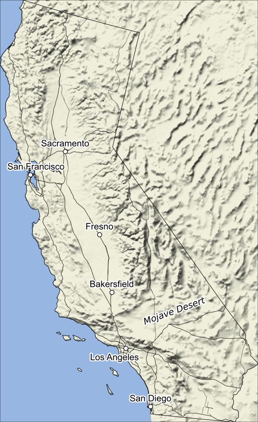
5980                                                                                             L. Bindle et al.: Stretched grids for GEOS-Chem

Table 1. Characteristics of various cubed-sphere grids and global latitude–longitude grids.

                                                                     no. of grid boxes                    Resolutionb
                                                                            per levela            Average                Range
                                 Cubed-sphere grids
                                 C24                                             3456              384 km        310–461 km
                                 C48                                            13 824             192 km        153–231 km
                                 C60                                            21 600             154 km        123–185 km
                                 C90                                            48 600             102 km         82–123 km
                                 C180                                          194 400              51 km          41–62 km
                                 C360                                          777 600              26 km          20–31 km
                                 Regular lat–long grids
                                 4◦ × 5◦                                         3600              376 km          88–472 km
                                 2◦ × 2.5◦                                      12 960             198 km          33–249 km
                                 1◦ × 1◦                                        64 800              89 km          10–111 km
                                 0.5◦ × 0.625◦                                 207 360              50 km            4–62 km
                                 0.25◦ × 0.3125◦                               829 440              25 km            2–31 km
                               a Number (no.) of grid boxes is listed for one vertical level. The GEOS-FP and MERRA-2
                               meteorological fields currently have 72 vertical levels. b Here we define the resolution of a grid
                               box as the square root of its area.

specifies a “target latitude”, Tφ , and “target longitude”, Tθ .                     The grid is refined up to the distance where L = 1 and coars-
The refinement is re-centered to these coordinates by rotat-                         ened at greater distances.
ing the grid.                                                                           Four scalar parameters fully describe a stretched grid: the
   Figure 2 illustrates the effect of S on stretching a cubed-                       size of the cubed sphere, the stretch factor (S), the target lat-
sphere grid. A stretch factor greater than 1 causes stretching.                      itude (Tφ ), and the target longitude (Tθ ). These concise pa-
Larger stretch factors cause more stretching and result in a                         rameters are conceptually simple, precise, and give the user
finer and more localized refinement. The resolution at the                           nimble control of the grid. The combination of cubed-sphere
center of the refinement is approximately S times finer than                         size and stretch factor controls the grid resolution. The target
it was before stretching, and the antipode resolution similarly                      latitude and longitude specify the center of the refined do-
is approximately S times coarser. These relative changes are                         main. Moderate stretch factors (e.g., 1.4–3.0) are suitable for
approximate since the Schmidt transform is continuous and                            broad refinements for continental-scale studies. Large stretch
the grid boxes have nonzero length edges. The grids in Fig. 2                        factors (e.g., > 5.0) are suitable for localized refinements for
illustrate three noteworthy features of stretched grids: (1) the                     regional-scale studies.
changes in resolution are smooth, (2) the refined domain di-
minishes as S increases, and (3) grid boxes outside the re-                          2.3     Choosing an appropriate stretch factor
fined domain expand. The cubed-sphere face at the center of
the refined domain is called the “target face”.                                      Although the stretch factor is a well-defined parameter, ap-
   The relative change to a grid box size from stretching can                        propriate values for atmospheric chemistry simulations will
be quantified by “local scaling”. This quantity represents the                       be application-specific and moderately variable. For compu-
effect of grid-stretching at a given point. For a stretch factor                     tational efficiency, it is desirable to use the largest viable
of S, the local scaling at a given point depends exclusively on                      stretch factor to achieve the finest refinement for a given
how far that point is from the target coordinate. Local scaling,                     cubed-sphere size. However, larger stretch factors also result
L, can be derived from Eq. (1), and expressed as                                     in a smaller refinement and in coarser resolutions outside the
                                                                                     refined domain. To determine the maximum suitable stretch
             1 + cos 2 + S 2 (1 − cos 2)                                             factor for a given application, one should consider the size of
L(2; S) =                                ,                   (2)
                         2S                                                          the domain that should be refined and the sensitivity of the
where 2 is the angular distance to the target point. Ap-                             study species to coarse resolutions outside the refinement. A
pendix B contains the derivation of Eq. (2). Figure 3 shows                          simple procedure for choosing a stretch factor, S, is choosing
local scaling as a function of distance, for stretch factors be-                     the maximum stretch factor subject to two constraints:
tween 1 and 10. Overlaid are dashed lines that show the lat-                            1. Constraining S by the size of the refined domain. Lo-
eral position of the face edges after stretching. In the target                            cal scaling is approximately constant and equal to 1/S
face, local scaling is approximately 1/S and nearly constant.                              throughout the target face. Therefore, defining the re-

Geosci. Model Dev., 14, 5977–5997, 2021                                                                     https://doi.org/10.5194/gmd-14-5977-2021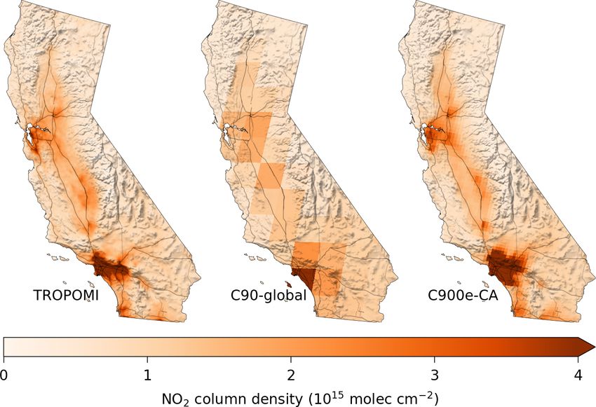
L. Bindle et al.: Stretched grids for GEOS-Chem                                                                                               5981

Figure 2. Three stretched grids that illustrate the effect of the stretch factor (S) on stretching a C16 cubed sphere. Local scaling is the relative
change to a grid box’s edge length induced by stretching.

                                                                                  where rE is Earth’s radius. Here, we define target-face
                                                                                  width, wtf , as the edge-to-edge distance across the cen-
                                                                                  ter of the face. For example, for a refined domain with
                                                                                  a diameter of at least 3000 km, the target face should be
                                                                                  at least 3000 km wide, and thus the stretch factor should
                                                                                  be less than or equal to 3.5. Alternatively, one could in-
                                                                                  spect Fig. 3 to find the distance from the target point to
                                                                                  the edge of the target face for a given value of S.

                                                                               2. Constraining S by a maximum and minimum resolution.
                                                                                  The target resolution is S 2 times finer than its antipode’s
                                                                                  resolution; therefore, a constraint for S based on the de-
                                                                                  sired maximum resolution, Rmax , and minimum resolu-
                                                                                  tion, Rmin , is
                                                                                       p
                                                                                  S ≤ Rmax /Rmin .                                         (4)

                                                                                  The minimum resolution, Rmin , is an important consid-
                                                                                  eration. Rmin imposes a limit on the coarsest resolution
                                                                                  outside of the refined domain. Therefore, the choice of
                                                                                  an appropriately fine Rmin can reduce potential bias in
Figure 3. Local scaling as a function of distance from the target                 species in the coarse grid outside of the refined domain
point, for stretch factors in the range 1–10. The dashed lines show               from affecting the study species in the refined domain.
the distance from the target point to the cubed-sphere face edges                 For example, for a maximum and minimum resolution
after stretching. The lower dashed line is the distance to the center             comparable to C360 and C24 cubed spheres, S ≤ 3.9, or
of the target face’s edges, and the upper dashed line is the distance
                                                                                  for a maximum and minimum resolution comparable to
to the center of the opposite face edges.
                                                                                  C360 and C48 cubed spheres, S ≤ 2.7.

                                                                            Once the constraints for S are determined, one can choose
     fined domain as the region where resolution is enhanced                S and the grid size for their simulation. For example, for a
     by a factor of ∼ S, the target face is a reasonable approx-            stretched grid with a refined domain with a diameter greater
     imation of the refined domain. For a target face with                  than 3000 km, a maximum resolution of C360, and a min-
     width greater than wtf , S must satisfy                                imum resolution of C24, the constraints would be S ≤ 3.5
                                                                            and S ≤ 3.9. To determine the grid size and stretch factor
                                                                            for a simulation from these constraints, first, assume S = 3.5
     S ≤ 0.414 cot (wtf /4 rE ) ,                                  (3)      as an initial value. For a maximum resolution comparable

https://doi.org/10.5194/gmd-14-5977-2021                                                         Geosci. Model Dev., 14, 5977–5997, 2021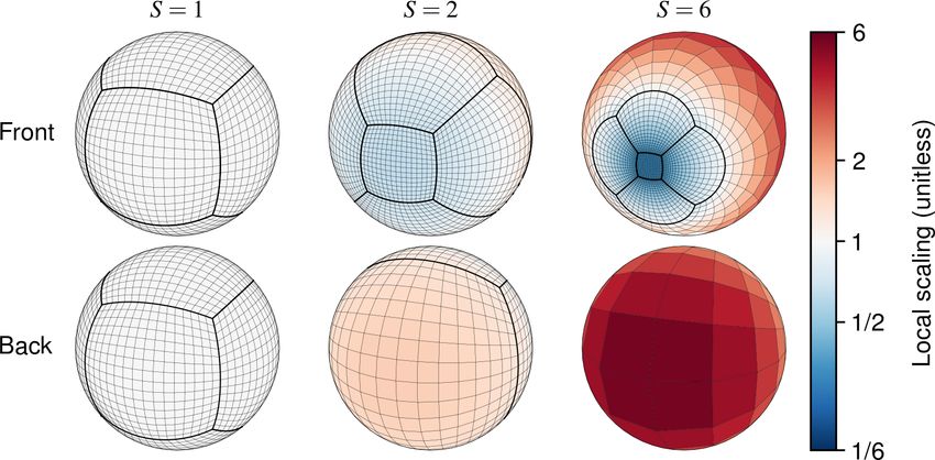
5982                                                                       L. Bindle et al.: Stretched grids for GEOS-Chem

to a C360 grid with S = 3.5, the grid size would be C102.9         being comparable to the resolution of a C180 cubed-sphere
(360/3.5 = 102.9). Since the grid size must be an even in-         grid.
teger, one should round up to C104 and choose S = 3.46
(360/104 = 3.46).                                                  2.5   Validating the stretched-grid capability
   The single refinement and the expansion of grid boxes
outside the refined domain are important limitations of grid-      Next, we test the implementation of stretched grid by
stretching. The coarse grid outside the refined domain is sus-     comparing the concentrations of oxidants and PM2.5 from
ceptible to resolution-dependent biases in O3 and CO (Wild         stretched-grid and cubed-sphere simulations. Prior tests were
and Prather, 2006; Yan et al., 2014, 2016), which could influ-     also conducted to identify and fix several technical errors
ence the representation of chemical processes in the refined       in some component capabilities. We choose the contigu-
domain. Therefore, the choice of an appropriately fine min-        ous US as the domain for this comparison and a standard
imum resolution is important (Rmin in constraint 2). Gener-        C96 cubed-sphere simulation to serve as the control simula-
ally, stretched-grid simulations are well suited for applica-      tion (C96-global). The stretched-grid simulation, C96e-NA,
tions that are principally sensitive to emissions and physical     has a grid size of C48 and stretching parameters S = 2.4,
processes in the refined domain. For example, stretched-grid       Tφ = 35◦ N, and Tθ = 96◦ W. The target point was chosen
simulations are well suited for regional studies of boundary       so that the target face approximately encompassed the popu-
layer concentrations of short-lived species. Applications such     lous regions of North America. The stretch factor was chosen
as evaluations of the global tropospheric O3 budget are better     so that the average resolution of C96e-NA was equal to the
suited for standard cubed-sphere simulations.                      average resolution of C96-global in the contiguous US; we
                                                                   note that the stretch factor is 2.4, rather than 2.0, because
2.4    Model configuration                                         the US is a region where the standard cubed-sphere grid has
                                                                   a finer resolution than its global average, as shown in Ap-
The simulations in this paper use a shared model configura-        pendix A. Figure 4 compares the resolution of C96e-NA and
tion of GCHP version 13.0.0-alpha.3. We use default emis-          C96-global grids.
sions for all species. Table 2 summarizes the emission in-            A consequence of the similar resolution of the C96-global
ventories that represent sources of NOx in the simulations.        and C94-global grids is that their grid boxes have little over-
Briefly, we use monthly anthropogenic emissions based on           lap; this makes their comparison sensitive to the precision
the National Emission Inventory (NEI) for 2011 with updated        of upscaling emissions (aliasing effects, i.e., differences in
annual scaling factors to account for changes in annual to-        upscaled emissions like NO point sources from differences
tals since 2011. In 2019, the scaling factor for NO was 0.61.      in how the grids cover a region). To calibrate an expec-
Biomass burning emissions are from the Global Fire Emis-           tation for these differences, we compare C96-global to a
sions Database version 4 (GFED4; van der Werf et al., 2017).       second standard cubed-sphere simulation, C94-global. We
Aircraft emissions are from the Aviation Emissions Inven-          choose C94-global because the similar resolution minimizes
tory Code (AEIC; Stettler et al., 2011). We use inventories        the frequency that its grid boxes overlap with the C96-global
for NOx emissions from soil microbial activity and lightning       grid boxes. Therefore, the comparison of C94-global and
calculated offline at the native resolution of the meteorol-       C96-global isolates differences from aliasing effects. The
ogy (Weng et al., 2020; The International GEOS-Chem User           frequency of grid box overlap between C96-global and
Community, 2019). Offline soil NOx emissions are based             C94-global is analogous to a beat frequency of 2; the regions
on the scheme described in Hudman et al. (2012), and of-           where overlap occurs is near the edges and across the center
fline lightning NOx emissions are based on the scheme de-          lines of the faces.
scribed in Murray et al. (2012). For meteorological data, we          Figure 5 compares C96e-NA with C96-global and
use GEOS-FP data because it offers superior horizontal res-        C94-global with C96-global. These comparisons are for the
olution data for advection input variables (0.25◦ × 0.3125◦ ).     fourth simulation month, to accommodate relaxation time for
All simulations use a 10 min time step for chemistry and a         CO and O3 (the simulations started 1 June 2018 and ran
5 min time step for transport.                                     through 1 October 2018). All three simulations used an iden-
   Simulations are named according to their grid. Standard         tical model configuration, apart from the grid, which is de-
cubed-sphere simulations are named by their resolution with        scribed in Sect. 2.4. The scatter near the surface is caused by
the suffix “-global”, referring to their resolution being quasi-   differences in the spatial allocation of emissions on different
uniform globally. For example, a standard C180 cubed-              grids (the precision of upscaling). Figure 5 shows that simu-
sphere simulation is named “C180-global”. Stretched-grid           lated averages from C96e-NA are consistent with C96-global
simulations are named according to their refinement effec-         and that their differences are comparable to the differences
tive resolution, with a suffix denoting the region that is re-     between two similar cubed-sphere simulations. We note a
fined. For example, a stretched-grid simulation with an ef-        small low bias in ozone above 400 hPa associated with non-
fective resolution of C180 in the contiguous US is named           linear chemical sensitivity to coarse grid boxes outside of the
“C180e-US”. “C180e” refers to the stretched-grid refinement        refined region. The C96e-NA grid resolution is coarser than

Geosci. Model Dev., 14, 5977–5997, 2021                                            https://doi.org/10.5194/gmd-14-5977-2021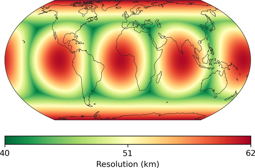
L. Bindle et al.: Stretched grids for GEOS-Chem                                                                                                   5983

Table 2. Emissions inventories in GEOS-Chem 13.0.0 that represent NOx sources in the simulations conducted in this paper.

                        Source type               Inventory               Resolution        Reference/notes
                        Anthropogenic
                           US                     NEI-2011               0.1◦ × 0.1◦        Annual totals are updated for 2018/19a
                           Asia                   MIX                 0.25◦ × 0.25◦         Li et al. (2017)
                           Global                 CEDSb                  0.5◦ × 0.5◦        McDuffie et al. (2020)
                        Lightning                 –                0.25 × 0.3125◦
                                                                        ◦                   Murray et al. (2012)
                        Soil                      –                0.25◦ × 0.3125◦          Weng et al. (2020)
                        Biomass burning           GFED4               0.25◦ × 0.25◦         van der Werf et al. (2017)
                        Aircraft                  AEIC                   1.0◦ × 1.0◦        Stettler et al. (2011)
                        Shipping                  CEDS                   0.5◦ × 0.5◦        McDuffie et al. (2020)
                      a Monthly fluxes, including diurnal and weekday–weekend variations and vertical allocations, based on criteria pollutants
                      National Tier 1 from https://www.epa.gov/air-emissions-inventories/air-pollutant-emissions-trends-data (last access: 8
                      May 2020). b Community Emissions Data System (CEDS)

                                                                                      tropospheric NO2 columns with observations. NO2 is cho-
                                                                                      sen because it is a well-measured species, and the sensitivity
                                                                                      of its simulated concentrations to model resolution and lo-
                                                                                      cal chemical and physical processes make it a prime exam-
                                                                                      ple of an application that is well suited for a stretched-grid
                                                                                      simulation. Here we explore two of the primary reasons one
                                                                                      might use the stretched-grid capability: (1) for a computa-
                                                                                      tionally efficient regional simulation and (2) to realize a finer
                                                                                      resolution than is otherwise possible. Section 3.1 considers
                                                                                      a comparison of columns in the contiguous US; columns
                                                                                      are simulated at ∼ 50 km resolution, with stretched-grid and
                                                                                      standard cubed-sphere simulations, to examine the ability of
                                                                                      a stretched-grid simulation to produce similar results to a
                                                                                      cubed-sphere simulation at a lesser computational expense.
                                                                                      Section 3.2 experiments with the use of a very large stretch
                                                                                      factor for a simulation targeting California with ∼ 10 km res-
                                                                                      olution and modest computational requirements.
                                                                                         We compare simulated tropospheric NO2 column densities
                                                                                      to retrieved column densities from TROPOMI. TROPOMI
                                                                                      is an instrument onboard the Sentinel-5P satellite launched
                                                                                      in 2018 into a sun-synchronous orbit with a local over-
Figure 4. Comparison of C96-global and C96e-NA grids. The top                         pass time of 13:30 LST (local solar time). TROPOMI in-
panels show the variability of resolution for both grids. The bottom                  cludes ultraviolet and visible band spectrometers. The re-
panel shows the grid face edges for C96-global and C96e-NA, with                      trieved NO2 column densities have 3.5 × 5.5 km2 resolution
the 125, 250, and 500 km resolution contours for C96e-NA.
                                                                                      and are calculated using a modified version of the Dutch
                                                                                      OMI NO2 (DOMINO) retrieval algorithm (Boersma et al.,
250 km in most of Asia, while the C96-global grid is finer                            2011, 2018). We include observations with retrieved cloud
than 125 km (Fig. 4). A finer grid size or a smaller stretch                          fractions less than 10 %. Retrieved NO2 column densities
factor could be used to increase resolution outside the refine-                       are sensitive to the a priori profiles used to calculate the air
ment if this type of bias is of concern for a stretched-grid                          mass factors (Boersma et al., 2018; Lorente et al., 2017).
application.                                                                          To avoid spurious differences from the retrieval a priori pro-
                                                                                      files when comparing simulated and retrieved NO2 column
                                                                                      densities, we recalculate the air mass factors with the mean
3   Stretched-grid case studies                                                       simulated relative vertical profiles (shape factors) from the
                                                                                      stretched-grid simulations following the approach described
Next, we demonstrate stretched-grid simulations with GCHP                             in Cooper et al. (2020) and Palmer et al. (2001). Evaluations
by conducting case studies in Sect. 3.1 and 3.2. The appli-                           of TROPOMI NO2 columns show good correlation with
cations we consider are regional comparisons of simulated                             ground-based measurements with a small low bias (Griffin

https://doi.org/10.5194/gmd-14-5977-2021                                                                       Geosci. Model Dev., 14, 5977–5997, 2021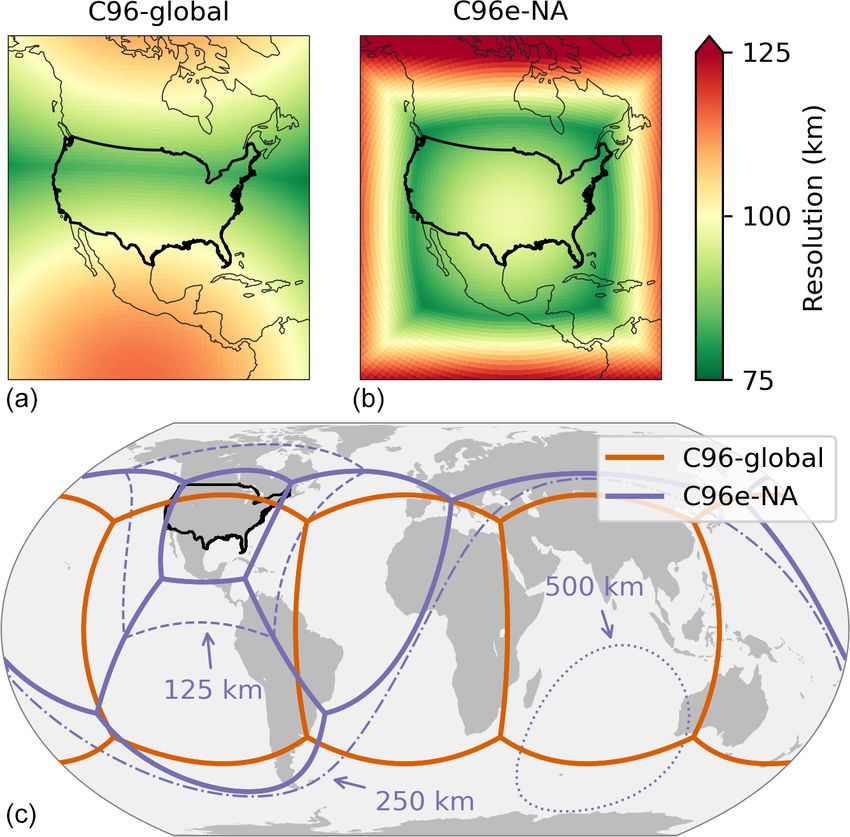
5984                                                                             L. Bindle et al.: Stretched grids for GEOS-Chem

                                                                        Figure 6. Comparison of C180-global and C180e-US grids. The top
                                                                        panels show the variability of resolution for both grids. The bottom
                                                                        panel shows the grid face edges for C180-global and C180e-US,
                                                                        with the 100, 250, and 500 km resolution contours for C180e-US.

                                                                        et al., 2019; Ialongo et al., 2020; Zhao et al., 2020; Tack et al.,
                                                                        2021).

                                                                        3.1   A stretched-grid simulation with a moderate
                                                                              stretch factor

                                                                        Here we consider a comparison of simulated and observed
                                                                        NO2 columns in the contiguous US. We compare simulated
                                                                        columns with ∼ 50 km resolution from stretched-grid and
                                                                        standard cubed-sphere simulations with observations from
                                                                        TROPOMI. Our focus is on the technical ability to use a
                                                                        stretched grid for an efficient fine-resolution simulation of
                                                                        the columns compared to using a standard cubed sphere for
                                                                        this purpose. The contiguous US is a large refinement do-
                                                                        main, and thus a moderate stretch factor is appropriate. This
                                                                        case is intended to be representative of a typical case where
                                                                        grid refinement is used in global models.
                                                                           For the cubed-sphere simulation, we use a C180 grid and
                                                                        refer to it as C180-global. For the stretched-grid simulation,
                                                                        we use a stretch factor of S = 3.0, a grid size of C60, and a
Figure 5. Comparison of simulated concentrations from C96e-NA           target point at 36◦ N, 99◦ W. We refer to the stretched-grid
with C96-global, and C94-global with C96-global. Points are 1-          simulation as C180e-US. The stretching parameters are cho-
month time averages for each grid box in the contiguous US for          sen so that the target face approximately encompasses the
the fourth simulation month (September 2018). The right column
                                                                        contiguous US. Figure 6 shows the resolution of the two
gauges expected differences due to the precision of upscaling emis-
                                                                        simulation grids. In the contiguous US, the average resolu-
sions to different grids. Concentrations in the lowermost model level
are shown in purple.                                                    tion of C180-global is 47.9 km, and the average resolution
                                                                        of C180e-US is 56.6 km. The total number of grid boxes in
                                                                        C180e-US is 9 times fewer than the number of grid boxes
                                                                        in C180-global (cf. C60 and C180 grids in Table 1). Both

Geosci. Model Dev., 14, 5977–5997, 2021                                                   https://doi.org/10.5194/gmd-14-5977-2021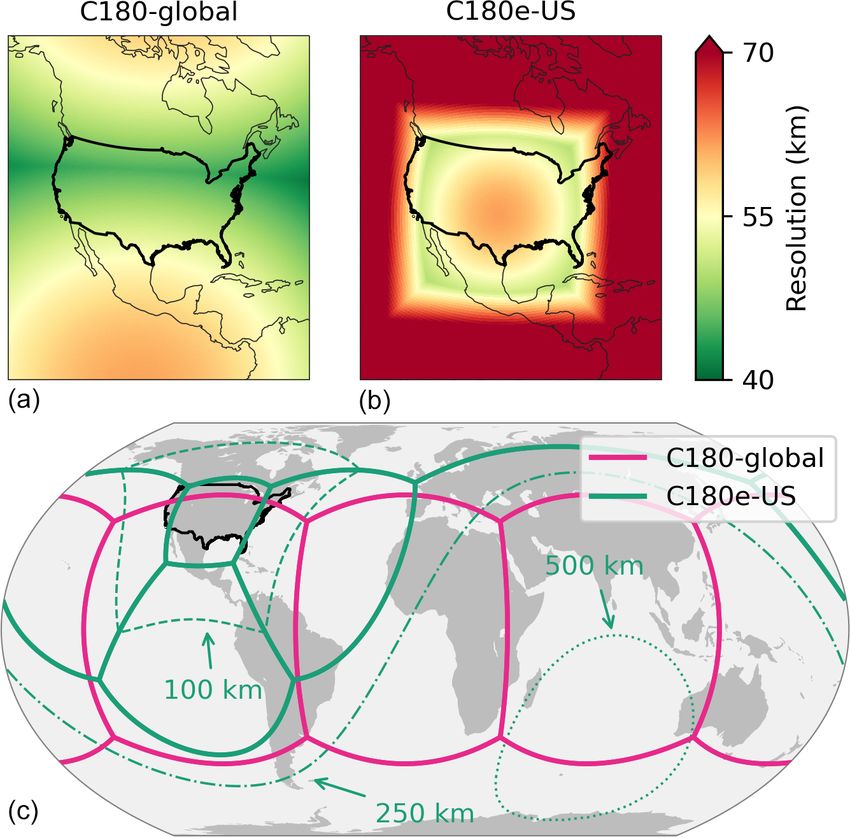
L. Bindle et al.: Stretched grids for GEOS-Chem                                                                                   5985

Figure 7. Mean tropospheric NO2 column densities from C180-global, C180e-US, C60-global, and TROPOMI observations for July 2019.
Simulated means only include points where TROPOMI observations were available. TROPOMI columns shown here use shape factors from
C180e-US. TROPOMI columns with shape factors from C180-global were nearly identical. An annotated map of the contiguous US is
provided in Fig. C1.

simulations use an identical model configuration, apart from
the grid. The model configuration is described in Sect. 2.4.
To examine C180e-US without grid-stretching, we conduct a
third simulation, C60-global.
   Figure 7 shows tropospheric NO2 column densities from
TROPOMI, C180-global, C180e-US, and C60-global for the
US in July 2019. All three simulations included a 1-month
spinup. An annotated map of the contiguous US is provided
in Fig. C1. The TROPOMI columns have high NO2 con-
centrations over major cities and low NO2 concentrations in
rural and remote regions. Simulated NO2 column densities
from C180-global and C180e-US are consistent throughout
the domain and generally capture the plumes over cities and
the low concentrations in rural and remote areas. Small dif-
ferences, like those seen near Four Corners and Denver, can
be attributed to differences from upscaling the emissions to
the simulation grids (i.e., aliasing). In the case of the differ-
ences near Four Corners, emissions from natural gas produc-
tion and power plants in the region have a spatial scale that is
finer than the simulation grids. C60-global failed to resolve
the local enhancements over major cities; a comparison with
C180e-US highlights the effectiveness of grid-stretching.           Figure 8. Comparison of C90-global and C900e-CA grids. The top
   The computational demands of C180e-US were signifi-              panels show the variability of resolution for both grids. The bottom
cantly less than C180-global and comparable to C60-global.          panel shows the grid face edges for C90-global and C900e-CA, with
                                                                    the 100, 500, and 1000 km resolution contours for C900e-CA.
Table 3 gives timing test results for C180-global, C180e-US,
and C60-global. In terms of total computational workload,
the total CPU time for C180e-US was ∼ 19 times less than

https://doi.org/10.5194/gmd-14-5977-2021                                               Geosci. Model Dev., 14, 5977–5997, 2021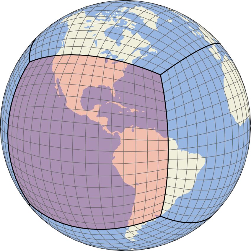
5986 L. Bindle et al.: Stretched grids for GEOS-Chem
Table 3. The 2-week timing test results comparing the computational expense of C180-global, C180e-US, and C60-global.
C180-global C180e-US C60-global
Number of cores used (CPUs) 384 48 48
Wall time
Chemistry (hours) 21.8 7.0 7.2
Dynamics (hours) 3.1 1.7 1.7
Data input (hours) 0.5 1.8 0.3
Other (hours) 0.3 0.2 0.2
Total wall time (hours) 25.7 10.7 9.4
Total CPU time (days) 411 21.3 18.7
Model throughput (days/day)∗ 13.1 31.4 35.7
∗ Simulation days per 24 wall hours.
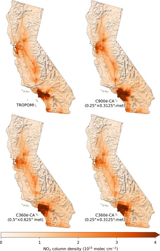
Figure 9. Mean tropospheric NO2 column densities from C90-global, C900e-CA, and TROPOMI observations for July 2019. Simulated
means only include points where TROPOMI observations were available. TROPOMI columns shown here use shape factors from C900e-CA.
An annotated map of California is provided in Fig. C2.
C180-global. The improvement is better than one would ap- 3.2 A stretched-grid simulation with a large stretch
proximate by simply considering the reduction in the total factor
number of grid boxes because the parallelization overhead is
reduced as well. In terms of model throughput, C180e-US A large stretch factor creates a grid with a strong but lo-
was 2.4 times faster than C180-global, despite using 8 times calized refinement. Here, we experiment with using a large
fewer cores. The total CPU time for C180e-US was 15 % stretch factor to simulate NO2 columns in California at
greater than C60-global. The slight increase of data input cost ∼ 10 km resolution. Simulated NO2 columns in California
in C180e-US is suspected to be caused by a load imbalance are known to be sensitive to model resolution because of sig-
in online input regridding in ESMF. Work to mitigate this nificant variability in emissions and topography (Valin et al.,
load imbalance is underway. 2011). This case study is intended to probe the computational
ability for very fine simulations and the feasibility of using a
highly stretched grid for an application that is well-suited for
stretching.
Geosci. Model Dev., 14, 5977–5997, 2021 https://doi.org/10.5194/gmd-14-5977-2021L. Bindle et al.: Stretched grids for GEOS-Chem 5987
For the stretched-grid simulation, we choose a grid size of small high-concentration features over Sacramento, Fresno,
C90 with stretching parameters S = 10, Tφ = 37.2◦ N, and and Bakersfield. The coarse resolution of C90-global fails
Tθ = 119.5◦ W. We refer to this simulation as C900e-CA. to resolve most spatial features seen in the TROPOMI and
The stretching parameters were chosen so that the target face C900e-CA columns and significantly underestimates high
approximately encompassed California. For comparison, we concentrations, except in Los Angeles (LA). The underes-
also conduct a cubed-sphere simulation with a C90 grid, timation of high concentrations in C90-global, such as in
which we refer to as C90-global. C90-global is effectively the San Francisco Bay Area, is associated with the aver-
C900e-CA without grid-stretching. Both simulations use an aging of fine-scale urban emissions over the coarse grid
identical model configuration, apart from the grid. Figure 8 boxes. A subtle feature in the TROPOMI columns is the
compares the resolution of the two simulation grids. The av- strong gradient along the LA Basin perimeter. Neither simu-
erage resolution of C900e-CA in California is 11.2 km. To lation captures this gradient well, and LA’s plume spuriously
understand the variability of the C900e-CA grid resolution it spreads into the Mojave Desert. The shallow inversion that
is useful to consider the local scaling at various locations. For prevents the plume from rising over the mountains might
example, New York is approximately 4000 km from C900e- be better represented in finer-resolution meteorological in-
CA’s target point. Figure 3 shows that for S = 10, the lo- puts that could better resolve coastal dynamics. Nonetheless,
cal scaling at 4000 km is close to 1. Equivalently, substitut- C900e-CA demonstrates a pronounced improvement over
ing S = 10 and 2 = 4000 km/rE in Eq. (2) gives L = 1.04. C90-global at resolving the challenging heterogeneity of Cal-
Therefore, the resolution of C900e-CA in New York is sim- ifornia with similar computational expense (within 17 %).
ilar to a standard C90 cubed sphere. This can be confirmed
in Fig. 8. The combination of a large stretch factor (S = 10)
and moderate grid size (C90) causes some grid boxes to be- 4 Conclusions
come very coarse. Grid boxes in the Indian Ocean and south-
Fine-resolution simulations of atmospheric chemistry are
eastern Africa are coarser than 1000 km. These coarse grid
necessary to capture fine-scale modes of variability such
boxes will result in an errors in O3 production and an over-
as localized sources, nonlinear chemistry, and boundary
estimation of stratosphere–troposphere exchange (Wild and
layer processes, but fine-resolution simulations have been
Prather, 2006). Therefore, the C900e-CA grid would not be
impeded by computational expense. This work developed
suitable for applications sensitive to O3 or CO in the mid-
stretched grids for the high-performance implementation of
troposphere and upper troposphere. This underscores that se-
GEOS-Chem (GCHP). The capability was validated against
lection of an appropriate stretched grid is application spe-
global cubed-sphere simulations. Applications were probed
cific.
with case studies that compared simulated concentrations
C900e-CA leverages the fine spatial resolution of an-
with observations from the TROPOMI satellite instrument.
thropogenic NO emissions data available for the US;
Stretched grids enable multiscale grids in GCHP while
the NEI-2011 inventory has a 0.1◦ × 0.1◦ grid (∼ 9 km).
complementing the other multiscale grid methods that are
C900e-CA uses meteorological data from the GEOS-FP
available in GEOS-Chem implementations. A primary bene-
data product with a spatial resolution of 0.25◦ × 0.3125◦
fit of grid-stretching is ease of use. The refinement is flexible
(∼ 25 km). We expect some of the detailed orographic and
and controlled by four simple runtime parameters. Stretched
coastal effects in California to be missed. C900e-CA identi-
grids operate naturally in GCHP, so switching between a
fies a need for even finer resolution of meteorological data,
stretched grid and cubed-sphere grid is seamless. Stretched-
for which there is ongoing work in the GCHP–GMAO com-
grid simulations are stand-alone simulations that do not re-
munity. In the regions where C900e-CA’s grid is finer than
quire any pregenerated or dynamically coupled boundary
the GEOS-FP data, the data are conservatively downscaled
conditions. Compared to nested grids, the main disadvan-
(online by ESMF). We evaluate the effect of using down-
tages of grid-stretching are that there is a single refinement
scaled meteorological data on the simulated NO2 columns in
and that one cannot control the refined domain, refinement
Appendix D and find no significant ill effects for our appli-
resolution, and global resolution independently.
cation.
Stretched-grid simulations can be used for regional- or
Figure 9 shows tropospheric NO2 column densities from
continental-scale simulation purposes. Generally, stretch fac-
TROPOMI, C900e-CA, and C90-global for California in
tors in the range 1.4–4.0 are applicable for large refined do-
July 2019. Both simulations used a 1-month spinup. An
mains. Higher stretch factors can be used for simulations at
annotated map of California is provided in Fig. C2. The
very fine resolution for regional-scale applications. To aid
TROPOMI columns have significant fine-scale variability
in choosing an appropriate stretch factor, we propose a sim-
throughout California; high concentrations over Los Ange-
ple procedure based on choosing the maximum stretch factor
les and in the San Francisco Bay Area; and smaller high-
subject to two constraints: the size of the refined domain and
concentration features over Sacramento, Fresno, and Bak-
the maximum and minimum resolution.
ersfield. C900e-CA resolves many of the fine-scale spa-
tial features seen in the TROPOMI columns, including the
https://doi.org/10.5194/gmd-14-5977-2021 Geosci. Model Dev., 14, 5977–5997, 20215988 L. Bindle et al.: Stretched grids for GEOS-Chem Computationally, stretched-grid simulations are capable of unprecedented spatial resolutions for GEOS-Chem. Fine- scale emissions, with accurate spatial and temporal variabil- ity, and meteorological inputs with fine horizontal, tempo- ral, and vertical resolution are needed to fully exploit these newly achievable resolutions. Stretched grids are publicly available and ready for scientific application in GEOS-Chem version 13.0.0. Appendix A: Variability of cubed-sphere grid resolution Figure A1 shows the variability of a C180 cubed-sphere grid’s resolution. The coarsest resolutions are at the center of faces, and the finest resolutions are at the corners of the faces. The average√resolution of a cubed-sphere grid can be approximated by AE / (6 × N × N ), where AE is the sur- face area of Earth (∼ 510 × 106 km2 ) and N is the size of the cubed sphere (e.g., N = 180 for a C180 grid). The average resolution of a C180 grid is 51 km. The resolution at the cen- ter of the face is 62 km, and the resolution at the corner of the face is 41 km. Figure A1. Variability of a C180 cubed sphere’s resolution. Geosci. Model Dev., 14, 5977–5997, 2021 https://doi.org/10.5194/gmd-14-5977-2021
L. Bindle et al.: Stretched grids for GEOS-Chem 5989
Appendix B: Derivation of local scaling
Local scaling, L, is the relative change to a grid box’s length
from grid stretching. Consider a line segment that follows
a meridian. The line segment starts at y and has length 1y.
After remapping the line segment with the Schmidt transform
(Eq. 1), the line segment starts at y 0 and has length 1y 0 . The
limit of the segment’s local scaling as 1y → 0 is equal to the
derivative of the Schmidt transform:
1y 0 φ 0 (y + 1y) − φ 0 (y)
L(y 0 ; S) = lim = lim
1y→0 1y 1y→0 1y
d 0
= φ (y). (B1)
dy
The derivative of the Schmidt transform is
d 0 2S
φ (y) = 2 , (B2)
dy S (1 − sin y) + sin y + 1
and thus the local scaling at y 0 is
2S
L(y 0 ; S) = . (B3)
S 2 (1 − sin y) + sin y + 1
We can obtain the local scaling at y, rather than y 0 , by sub-
stituting the inverse of the Schmidt transform into Eq. (B3).
This gives
S 2 (1 + sin y) − sin y + 1
L(y; S) = . (B4)
2S
Finally, we can generalize Eq. (B4) so it is a function of ar-
clength from the target. The center of the refinement after ap-
plying Eq. (1) is at the South Pole. The arclength from y to
the South Pole is 2 = y −(−π/2). Substituting y = 2−π/2
into Eq. (B4) gives
S 2 (1 − cos 2) + cos 2 + 1
L(2; S) = . (B5)
2S
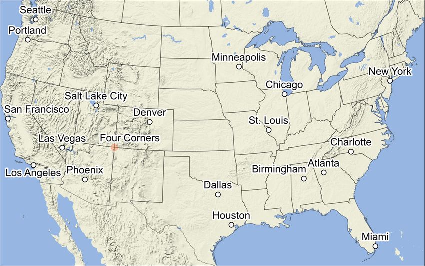
https://doi.org/10.5194/gmd-14-5977-2021 Geosci. Model Dev., 14, 5977–5997, 20215990 L. Bindle et al.: Stretched grids for GEOS-Chem Appendix C: Maps of locations discussed in the text Figure C1 shows a map of the contiguous US. Locations that are discussed in the text and locations with notable features in Fig. 7 are marked. Figure C2 shows a map of California. Locations that are discussed in the text and locations with notable features in Fig. 9 are marked. Figure C1. Map of the contiguous US. Locations discussed in the text and locations with notable features in Fig. 7 are marked. Geosci. Model Dev., 14, 5977–5997, 2021 https://doi.org/10.5194/gmd-14-5977-2021
L. Bindle et al.: Stretched grids for GEOS-Chem                                                                               5991

Figure C2. Map of the California. Locations discussed in the text and locations with notable features in Fig. 9 are marked.

https://doi.org/10.5194/gmd-14-5977-2021                                                    Geosci. Model Dev., 14, 5977–5997, 2021
5992                                                            L. Bindle et al.: Stretched grids for GEOS-Chem

Appendix D: Evaluation of interpolating meteorological
inputs in California NO2 simulation

Section 3.2 demonstrates the use of a stretched-grid simu-
lation for simulating tropospheric NO2 column densities in
California. The simulation, C900e-CA, has an average reso-
lution of 11.2 km in California, which is approximately twice
as fine as the input meteorological data (0.25◦ × 0.3125◦
grid, or ∼ 25 km resolution). To check that interpolating
meteorological data in C900e-CA does not have signifi-
cant unexpected consequences, we downscaled the data to
a 0.5◦ × 0.625◦ grid (∼ 50 km) and conducted a pair of
stretched-grid simulations with ∼ 25 km resolution; one used
the 0.25◦ × 0.3125◦ data, and the other used the downscaled
0.5◦ × 0.625◦ data. The NO2 columns from these simulations
are shown in Fig. D1 (second row), along with the columns
from TROPOMI and C900e-CA (first row). The grid for
these simulations was a C60 cubed sphere with a stretch
factor of S = 6 (∼ 25 km) and a target point of 37.2◦ N,
119.5◦ W (same as C900e-CA). Both used a 1-month spinup.
Comparison of the lower panels in Fig. D1 shows that in-
terpolating the 0.5◦ × 0.625◦ meteorological inputs to the
∼ 25 km grid has little effect on the simulated NO2 columns.
This suggests the consequences of interpolating meteorolog-
ical data in C900e-CA are minor for our application and that
the variability is driven by the resolution of emissions data
(∼ 9 km resolution).

Geosci. Model Dev., 14, 5977–5997, 2021                               https://doi.org/10.5194/gmd-14-5977-2021
L. Bindle et al.: Stretched grids for GEOS-Chem                                                                        5993

Figure D1. Mean tropospheric NO2 column densities from TROPOMI, C900e-CA, C360e-CA with 0.25◦ × 0.3125◦ meteorological data,
and C360e-CA with meteorological data downscaled to 0.5◦ × 0.625◦ .

https://doi.org/10.5194/gmd-14-5977-2021                                         Geosci. Model Dev., 14, 5977–5997, 2021
5994                                                                           L. Bindle et al.: Stretched grids for GEOS-Chem

Code availability. GEOS-Chem is an open source project dis-           References
tributed under the MIT License at https://github.com/geoschem/
GCHP (last access: 28 June 2021). The exact version of GCHP           Allen, D., Pickering, K., Stenchikov, G., Thompson, A., and Kondo,
used in this paper was 13.0.0-alpha.3 and is archived on Zenodo         Y.: A three-dimensional total odd nitrogen (NOy) simulation dur-
(https://doi.org/10.5281/zenodo.4317978, The International GEOS-        ing SONEX using a stretched-grid chemical transport model, J.
Chem User Community, 2020).                                             Geophys. Res.-Atmos., 105, 3851–3876, 2000.
                                                                      Bey, I., Jacob, D. J., Yantosca, R. M., Logan, J. A., Field,
                                                                        B. D., Fiore, A. M., Li, Q., Liu, H. Y., Mickley, L. J.,
Data availability. The simulations in this paper use default GEOS-      and Schultz, M. G.: Global modeling of tropospheric chem-
Chem 13.0 emissions and meteorological data that can be obtained        istry with assimilated meteorology: Model description and
from the GEOS-Chem input data repository: http://geoschemdata.          evaluation, J. Geophys. Res.-Atmos., 106, 23073–23095,
wustl.edu/ExtData/ (last access: 4 October 2021). The instructions      https://doi.org/10.1029/2001JD000807, 2001.
for downloading the input data for GEOS-Chem 13.0 from the data       Boersma, K., Braak, R., and van der A, R. J.: Dutch OMI
repository are given in the GEOS-Chem 13.0 User Guide (https:           NO2 (DOMINO) data product v2. 0, Tropospheric Emis-
//gchp.readthedocs.io, last access: 8 October 2021).                    sions Monitoring Internet Service on-line documentation, avail-
                                                                        able at: http://www.temis.nl/docs/OMI_NO2_HE5_2.0_2011.
                                                                        pdf (last access: 5 July 2020), 2011.
                                                                      Boersma, K. F., Eskes, H. J., Richter, A., De Smedt, I., Lorente,
Author contributions. LB implemented and validated the stretched-
                                                                        A., Beirle, S., van Geffen, J. H. G. M., Zara, M., Peters, E.,
grid capability in GCHP. RVM, DJJ, and SP provided project over-
                                                                        Van Roozendael, M., Wagner, T., Maasakkers, J. D., van der
sight and top-level design. MJC reprocessed TROPOMI columns
                                                                        A, R. J., Nightingale, J., De Rudder, A., Irie, H., Pinardi,
with shape factors from simulations. EWL, LB, and SDE performed
                                                                        G., Lambert, J.-C., and Compernolle, S. C.: Improving algo-
MAPL 2 upgrade in GCHP. BMA and TLC developed stretched-
                                                                        rithms and uncertainty estimates for satellite NO2 retrievals: re-
grid capability in MAPL 2. WMP developed FV3. HW, JL, LTM,
                                                                        sults from the quality assurance for the essential climate vari-
and JM developed grid-independent emissions for GEOS-Chem,
                                                                        ables (QA4ECV) project, Atmos. Meas. Tech., 11, 6651–6678,
and CAK developed HEMCO. LB wrote the manuscript. All au-
                                                                        https://doi.org/10.5194/amt-11-6651-2018, 2018.
thors contributed to manuscript editing and revisions.
                                                                      Cooper, M. J., Martin, R. V., McLinden, C. A., and Brook, J. R.:
                                                                        Inferring ground-level nitrogen dioxide concentrations at fine
                                                                        spatial resolution applied to the TROPOMI satellite instrument,
Competing interests. The authors declare that they have no conflict     Environ. Res. Lett., 15, 104013, https://doi.org/10.1088/1748-
of interest.                                                            9326/aba3a5, 2020.
                                                                      Courtier, P. and Geleyn, J.-F.: A global numerical weather predic-
                                                                        tion model with variable resolution: Application to the shallow-
Disclaimer. Publisher’s note: Copernicus Publications remains           water equations, Q. J. Roy. Meteor. Soc., 114, 1321–1346, 1988.
neutral with regard to jurisdictional claims in published maps and    Davis, D. D., Grodzinsky, G., Kasibhatla, P., Crawford, J., Chen,
institutional affiliations.                                             G., Liu, S., Bandy, A., Thornton, D., Guan, H., and Sandholm,
                                                                        S.: Impact of ship emissions on marine boundary layer NO x and
                                                                        SO 2 Distributions over the Pacific Basin, Geophys. Res. Lett.,
Acknowledgements. We are grateful to the Research Infrastructure        28, 235–238, https://doi.org/10.1029/2000GL012013, 2001.
Service (RIS) at Washington University in St. Louis for providing     Eastham, S. D., Weisenstein, D. K., and Barrett, S. R.:
computing resources. The meteorological data (GEOS-FP) used in          Development and evaluation of the unified tropospheric–
this study have been provided by the Global Modeling and Assim-         stratospheric chemistry extension (UCX) for the global
ilation Office (GMAO) at NASA Goddard Space Flight Center. We           chemistry-transport model GEOS-Chem, Atmos. Environ., 89,
thank the two anonymous reviewers for their constructive comments       52–63, https://doi.org/10.1016/j.atmosenv.2014.02.001, 2014.
and suggestions.                                                      Eastham, S. D., Long, M. S., Keller, C. A., Lundgren, E., Yan-
                                                                        tosca, R. M., Zhuang, J., Li, C., Lee, C. J., Yannetti, M., Auer,
                                                                        B. M., Clune, T. L., Kouatchou, J., Putman, W. M., Thompson,
Financial support. This research has been supported by the Earth        M. A., Trayanov, A. L., Molod, A. M., Martin, R. V., and Ja-
Sciences Division (grant no. AIST-18-0011) and the Natural              cob, D. J.: GEOS-Chem High Performance (GCHP v11-02c):
Sciences and Engineering Research Council of Canada (grant              a next-generation implementation of the GEOS-Chem chemi-
no. RGPIN-2019-04670).                                                  cal transport model for massively parallel applications, Geosci.
                                                                        Model Dev., 11, 2941–2953, https://doi.org/10.5194/gmd-11-
                                                                        2941-2018, 2018.
Review statement. This paper was edited by Fiona O’Connor and         Feng, X., Lin, H., and Fu, T.-M.: WRF-GC: online two-way
reviewed by two anonymous referees.                                     coupling of WRF and GEOS-Chem for regional atmospheric
                                                                        chemistry modeling, EGU General Assembly 2020, Online, 4–8
                                                                        May 2020, EGU2020-5165, https://doi.org/10.5194/egusphere-
                                                                        egu2020-5165, 2020
                                                                      Fox-Rabinovitz, M., Côté, J., Dugas, B., Déqué, M., and McGregor,
                                                                        J. L.: Variable resolution general circulation models: Stretched-

Geosci. Model Dev., 14, 5977–5997, 2021                                                 https://doi.org/10.5194/gmd-14-5977-2021
L. Bindle et al.: Stretched grids for GEOS-Chem 5995
grid model intercomparison project (SGMIP), J. Geophys. Res., ground-based measurements in Helsinki, Atmos. Meas. Tech.,
111, D16104, https://doi.org/10.1029/2005JD006520, 2006. 13, 205–218, https://doi.org/10.5194/amt-13-205-2020, 2020.
Fox-Rabinovitz, M., Cote, J., Dugas, B., Deque, M., McGre- Keller, C. A., Long, M. S., Yantosca, R. M., Da Silva, A.
gor, J. L., and Belochitski, A.: Stretched-grid Model Intercom- M., Pawson, S., and Jacob, D. J.: HEMCO v1.0: a ver-
parison Project: decadal regional climate simulations with en- satile, ESMF-compliant component for calculating emissions
hanced variable and uniform-resolution GCMs, Meteorol. At- in atmospheric models, Geosci. Model Dev., 7, 1409–1417,
mos. Phys., 100, 159–178, https://doi.org/10.1007/s00703-008- https://doi.org/10.5194/gmd-7-1409-2014, 2014.
0301-z, 2008. Kim, S.-W., Natraj, V., Lee, S., Kwon, H.-A., Park, R., de Gouw, J.,
Freitas, S. R., Longo, K. M., Chatfield, R., Latham, D., Silva Dias, Frost, G., Kim, J., Stutz, J., Trainer, M., Tsai, C., and Warneke,
M. A. F., Andreae, M. O., Prins, E., Santos, J. C., Gielow, R., C.: Impact of high-resolution a priori profiles on satellite-based
and Carvalho Jr., J. A.: Including the sub-grid scale plume rise of formaldehyde retrievals, Atmos. Chem. Phys., 18, 7639–7655,
vegetation fires in low resolution atmospheric transport models, https://doi.org/10.5194/acp-18-7639-2018, 2018.
Atmos. Chem. Phys., 7, 3385–3398, https://doi.org/10.5194/acp- Krinner, G., Genthon, C., Li, Z.-X., and Le Van, P.: Studies of the
7-3385-2007, 2007. Antarctic climate with a stretched-grid general circulation model,
Garcia-Menendez, F. and Odman, M. T.: Adaptive grid use in air J. Geophys. Res.-Atmos., 102, 13731–13745, 1997.
quality modeling, Atmosphere, 2, 484–509, 2011. Krol, M., Houweling, S., Bregman, B., van den Broek, M., Segers,
Garcia-Menendez, F., Yano, A., Hu, Y., and Odman, M. T.: An A., van Velthoven, P., Peters, W., Dentener, F., and Bergamaschi,
adaptive grid version of CMAQ for improving the resolution of P.: The two-way nested global chemistry-transport zoom model
plumes, Atmos. Pollut. Res., 1, 239–249, 2010. TM5: algorithm and applications, Atmos. Chem. Phys., 5, 417–
Goldberg, D. L., Lamsal, L. N., Loughner, C. P., Swartz, W. H., 432, https://doi.org/10.5194/acp-5-417-2005, 2005.
Lu, Z., and Streets, D. G.: A high-resolution and observation- Li, J., Wang, Y., and Qu, H.: Dependence of Summertime Surface
ally constrained OMI NO2 satellite retrieval, Atmos. Chem. Ozone on NOx and VOC Emissions Over the United States:
Phys., 17, 11403–11421, https://doi.org/10.5194/acp-17-11403- Peak Time and Value, Geophys. Res. Lett., 46, 3540–3550,
2017, 2017. https://doi.org/10.1029/2018GL081823, 2019.
Goto, D., Dai, T., Satoh, M., Tomita, H., Uchida, J., Misawa, S., Li, M., Zhang, Q., Kurokawa, J.-I., Woo, J.-H., He, K., Lu, Z.,
Inoue, T., Tsuruta, H., Ueda, K., Ng, C. F. S., Takami, A., Sugi- Ohara, T., Song, Y., Streets, D. G., Carmichael, G. R., Cheng,
moto, N., Shimizu, A., Ohara, T., and Nakajima, T.: Application Y., Hong, C., Huo, H., Jiang, X., Kang, S., Liu, F., Su, H.,
of a global nonhydrostatic model with a stretched-grid system to and Zheng, B.: MIX: a mosaic Asian anthropogenic emission
regional aerosol simulations around Japan, Geosci. Model Dev., inventory under the international collaboration framework of
8, 235–259, https://doi.org/10.5194/gmd-8-235-2015, 2015. the MICS-Asia and HTAP, Atmos. Chem. Phys., 17, 935–963,
Griffin, D., Zhao, X., McLinden, C. A., Boersma, F., Bourassa, https://doi.org/10.5194/acp-17-935-2017, 2017.
A., Dammers, E., Degenstein, D., Eskes, H., Fehr, L., Fiole- Li, Y., Henze, D. K., Jack, D., and Kinney, P. L.: The influence of
tov, V., Hayden, K., Kharol, S. K., Li, S., Makar, P., Mar- air quality model resolution on health impact assessment for fine
tin, R. V., Mihele, C., Mittermeier, R. L., Krotkov, N., Sneep, particulate matter and its components, Air Qual. Atmos. Hlth., 9,
M., Lamsal, L. N., Linden, M. t., Geffen, J. v., Veefkind, P., 51–68, https://doi.org/10.1007/s11869-015-0321-z, 2016.
and Wolde, M.: High-Resolution Mapping of Nitrogen Diox- Li, Y., Pickering, K. E., Barth, M. C., Bela, M. M., Cummings,
ide With TROPOMI: First Results and Validation Over the K. A., and Allen, D. J.: Evaluation of Parameterized Convec-
Canadian Oil Sands, Geophys. Res. Lett., 46, 1049–1060, tive Transport of Trace Gases in Simulation of Storms Observed
https://doi.org/10.1029/2018GL081095, 2019. During the DC3 Field Campaign, J. Geophys. Res.-Atmos., 123,
Harris, L. M., Lin, S.-J., and Tu, C.: High-Resolution Climate Sim- 11238–11261, https://doi.org/10.1029/2018JD028779, 2018.
ulations Using GFDL HiRAM with a Stretched Global Grid, Lin, H., Feng, X., Fu, T.-M., Tian, H., Ma, Y., Zhang, L., Ja-
J. Climate, 29, 4293–4314, https://doi.org/10.1175/JCLI-D-15- cob, D. J., Yantosca, R. M., Sulprizio, M. P., Lundgren, E.
0389.1, 2016. W., Zhuang, J., Zhang, Q., Lu, X., Zhang, L., Shen, L., Guo,
Heckel, A., Kim, S.-W., Frost, G. J., Richter, A., Trainer, M., and J., Eastham, S. D., and Keller, C. A.: WRF-GC (v1.0): online
Burrows, J. P.: Influence of low spatial resolution a priori data coupling of WRF (v3.9.1.1) and GEOS-Chem (v12.2.1) for re-
on tropospheric NO2 satellite retrievals, Atmos. Meas. Tech., 4, gional atmospheric chemistry modeling – Part 1: Description
1805–1820, https://doi.org/10.5194/amt-4-1805-2011, 2011. of the one-way model, Geosci. Model Dev., 13, 3241–3265,
Hill, C., DeLuca, C., Balaji, Suarez, M., and Da Silva, https://doi.org/10.5194/gmd-13-3241-2020, 2020.
A.: The Architecture of the Earth System Mod- Long, M. S., Yantosca, R., Nielsen, J. E., Keller, C. A., da
eling Framework, Comput. Sci. Eng., 6, 18–28, Silva, A., Sulprizio, M. P., Pawson, S., and Jacob, D. J.:
https://doi.org/10.1109/MCISE.2004.1255817, 2004. Development of a grid-independent GEOS-Chem chemical
Hudman, R. C., Moore, N. E., Mebust, A. K., Martin, R. V., Russell, transport model (v9-02) as an atmospheric chemistry module
A. R., Valin, L. C., and Cohen, R. C.: Steps towards a mechanistic for Earth system models, Geosci. Model Dev., 8, 595–602,
model of global soil nitric oxide emissions: implementation and https://doi.org/10.5194/gmd-8-595-2015, 2015.
space based-constraints, Atmos. Chem. Phys., 12, 7779–7795, Lorente, A., Folkert Boersma, K., Yu, H., Dörner, S., Hilboll, A.,
https://doi.org/10.5194/acp-12-7779-2012, 2012. Richter, A., Liu, M., Lamsal, L. N., Barkley, M., De Smedt, I.,
Ialongo, I., Virta, H., Eskes, H., Hovila, J., and Douros, J.: Compar- Van Roozendael, M., Wang, Y., Wagner, T., Beirle, S., Lin, J.-
ison of TROPOMI/Sentinel-5 Precursor NO2 observations with T., Krotkov, N., Stammes, P., Wang, P., Eskes, H. J., and Krol,
M.: Structural uncertainty in air mass factor calculation for NO2
https://doi.org/10.5194/gmd-14-5977-2021 Geosci. Model Dev., 14, 5977–5997, 2021You can also read