Hardware Adaptive High-Order Interpolation for Real-Time Graphics
←
→
Page content transcription
If your browser does not render page correctly, please read the page content below
High-Performance Graphics 2021                                                                                                          Volume 40 (2021), Number 8
N. Binder and T. Ritschel
(Guest Editors)

                              Hardware Adaptive High-Order Interpolation
                                       for Real-Time Graphics

                                                                       1                  2                   1
                                                              D. Lin       and L. Seiler        and C. Yuksel
                                                                                1
                                                                                  University of Utah
                                                                            2
                                                                                Facebook Reality Labs

         Abstract
         Interpolation is a core operation that has widespread use in computer graphics. Though higher-order interpolation provides
         better quality, linear interpolation is often preferred due to its simplicity, performance, and hardware support.
         We present a unified refactoring of quadratic and cubic interpolations as standard linear interpolation plus linear interpo-
         lations of higher-order terms and show how they can be applied to regular grids and (triangular/tetrahedral) simplexes Our
         formulations can provide significant reduction in computation cost, as compared to typical higher-order interpolations and
         prior approaches that utilize existing hardware linear interpolation support to achieve higher-order interpolation. In addition,
         our formulation allows approximating the results by dynamically skipping some higher order terms with low weights for further
         savings in both computation and storage. Thus, higher-order interpolation can be performed adaptively, as needed.
         We also describe how relatively minor modifications to existing GPU hardware could provide hardware support for quadratic
         and cubic interpolations using our approach for both texture filtering operations and barycentric interpolation.
         We present a variety of examples using triangular, rectangular, tetrahedral, and cuboidal interpolations, showing the effective-
         ness of our higher-order interpolations in different applications.
         CCS Concepts
         • Computing methodologies → Graphics processors; Texturing;

1. Introduction                                                                               in 2D and 3D domains. We also explain how this approach can be
                                                                                              extended to interpolation in a simplex (triangles and tetrahedrons).
Parameter interpolation is widely used in computer graphics. Most
commonly, it is performed linearly (i.e. bilinearly in 2D and trilin-                            Our formulations require less computation than standard high-
early in 3D). For example, 2D texture sampling on the GPU uses                                order interpolation approaches and the state-of-art high-order inter-
bilinear interpolation to blend the color of the nearest four pixels,                         polation methods performed on existing hardware [Csé18]. In ad-
and shading normal (or any other attribute on a triangle) is com-                             dition, it is suitable for an efficient hardware implementation that
puted using a linear combination of the three triangle vertex nor-                            requires relatively minor changes to existing linear interpolation
mals (or attributes).                                                                         pipeline on today’s GPUs, as we describe.
  However, linear interpolation is prone to visual artifacts like                                Moreover, it allows clamping high-order difference terms when
Mach bands. Such problems can be resolved with high-order inter-                              they are below a threshold, saving a sizeable amount of computa-
polations, such as quadratic or cubic, which are known to provide                             tion when high frequency details are sparse. This leads to an adap-
superior quality.                                                                             tive high-order interpolation solution, which incurs additional com-
                                                                                              putation over linear interpolation only when needed.
   Yet, lack of hardware support for high-order interpolation makes
it undesirable for real-time graphics applications with limited com-                             In applications not suitable for a hardware implementation, our
putation budgets. This can be attributed to the computation cost                              formulation allows skipping additional storage of high-order data,
of high-order interpolation and the significant hardware changes                              saving substantial amount of storage and computation cost.
needed for supporting them directly.
                                                                                                 We show examples in a wide range of real-time graphics ren-
   In this paper, we present a unified mathematical formulation that                          dering domains to show that our adaptive high-order interpolation
covers quadratic and cubic interpolation, expressing them as linear                           with our proposed hardware can significantly improve visual qual-
interpolation plus some high-order difference terms. This provides                            ity, using only 1× to 2× more computation than linear interpolation
a simpler form than common high-order interpolation formulations                              in typical cases. Note that this is significantly cheaper than 5× to

© 2021 The Author(s)
Computer Graphics Forum © 2021 The Eurographics Association and John
Wiley & Sons Ltd. Published by John Wiley & Sons Ltd.
D. Lin & L. Seiler & C. Yuksel / Hardware Adaptive High-Order Interpolation for Real-Time Graphics

7× more computation required by the state-of-art high-order inter-              Numerous works have proposed FPGA implementation of cu-
polation on existing hardware [Csé18; Csé19].                                bic interpolation. Due to the high computational complexity of
                                                                             bicubic interpolation, a direct FPGA implementation of bicubic
   We begin by providing the background and related prior work
                                                                             interpolation requires a lot of hardware resources [NA05]. To re-
in Section 2. In Section 3 we describe our high-order interpolation
                                                                             duce the computational complexity, many FPGA implementations
formulations in grids and explain how they can be used in prac-
                                                                             [LSC*08; WDLY11; GNSS14] limit the scope to handle specific
tical applications, such as texture filtering. Section 4 presents the
                                                                             image operation like scaling, where the bicubic weight pattern is
details of how the existing hardware texture filtering pipeline can
                                                                             repeated across the whole image and only needs to be computed
be modified to provide support for our high-order interpolation for-
                                                                             once. Orthogonal methods like quantizing the interpolation weights
mulations. Then, in Section 5 we describe our high-order interpola-
                                                                             [ZLZ*10], approximating the cubic kernel with multiple piecewise
tions for simplexes, such as triangles and tetrahedra. Possible hard-
                                                                             linear function [LSC*10; GNSS14], and using a mixture of cubic
ware acceleration techniques for simplex meshes are described in
                                                                             and linear function [BBGB20] have been applied in FPGA imple-
Section 6. We present our evaluation and results in Section 7 and
                                                                             mentations. Sanaullah et al. [SKH16] presented an FPGA imple-
conclude in Section 8.
                                                                             mentation of tricubic interpolation for molecular dynamics simula-
                                                                             tions. In comparison to these FPGA implementations, our method
2. Related Work                                                              adaptively reduces the computational cost, and only requires slight
                                                                             modification to the existing GPU. Thus, our method can easily uti-
Before we discuss the details of our approach, we summarize the              lize the power of existing texture units to provide high order inter-
related prior work in this section.                                          polation for a wide range of graphics applications.
                                                                                A graphics workstation system [MBDM97] has been made to
2.1. Interpolation for Grids of Data                                         support hardware bicubic interpolation at half of the rate of trilin-
                                                                             ear interpolation [Map06]. However, modern GPUs do not provide
Many graphics applications require reconstructing smooth signals             extra hardware to support higher-order filtering. Hardware imple-
from (1D, 2D, or 3D) grids of data, usually stored as images or              mentations of higher-order filtering into standard GPU texture units
textures. For that, reconstruction filters are required. Bilinear or         cannot be justified if they require a large amount of dedicated logic
trilinear interpolation provides a cheap way to generate continu-            that could instead be devoted to performing more bilinear interpo-
ous signal out of discrete samples and they are supported by most            lations per clock. Proposals to reuse existing texture logic require at
graphics hardware. Yet, cubic interpolation is known to signifi-             least four bilinear texture reads per sample, plus shader execution
cantly improve the quality of texture filtering [SH05], volume ren-          time to select the bilinear sample positions [SH05; Csé18].
dering [ML94], and temporal anti-aliasing [YLS20].
                                                                                There is a category of adaptive interpolation techniques [MH15]
   Keys [Key81] introduced a family of cubic cardinal splines that           for image resizing that derives interpolation weights from local
interpolates the sampling data. Mitchell and Netravali [MN88] de-            spatial features (e.g. edge orientation statistics) of the images to
rived BC-splines to describe a more general family of cubic re-              provide better visual quality than bicubic interpolation. However,
construction filters that may or may not interpolate the data. The           these methods generally involve expensive computation and are
family of splines is parameterized by B and C. All cardinal splines          highly specified for the task of image resizing. In comparison, our
have B=0. A separable bicubic filter using the BC-spline family has          approach is similar to the hierarchical form of high-order FEM
been implemented in shader code [Bjo04] to provide high quality              [ZTZ05], where the difference between the higher-order element
image magnification filtering. Sigg and Hadwiger [SH05] proposed             node values and lower-order element interpolation results are used
refactoring a bicubic/tricubic B-Spline filter (B=1,C=0), into a lin-        as part of the high-order element. We adaptively discard small high-
ear combination of four/eight hardware bilinear/trilinear taps.              order terms purely based on the mathematical formulation of bicu-
                                                                             bic (and other high-order) interpolation. Our method is targeted
   By modulating the source image with a checkerboard pattern,               at improving the performance of high order interpolation, and our
Csébfalvi [Csé18] solves the problem of negative bilinear/trilinear          method handles a wide range of applications in real-time rendering.
weights, allowing Catmull-Rom spline filter to be partially accel-
erated by hardware in a similar way. Since Catmull-Rom spline
(B=0,C=1/2) interpolates the original data, it does not have the             2.2. Interpolation for Simplexes
over-blurring problem of B-Spline filters. In a survey by Moller             Triangles and tetrahedrons are common building blocks of com-
at al. [MMMY97], Catmull-Rom splines are verified to achieve the             puter graphics. Shading a triangular mesh relies on interpolating
lowest reconstruction error in the entire family of BC-Spline filters.       vertex attributes, such asposition, normal, and texture coordinates.
                                                                             Linear interpolation of triangle vertex attributes are widely sup-
   More recently, Csébfalvi [Csé19] proposed a method that uses
                                                                             ported by graphics hardware.
hardware trilinear interpolation results for gradient estimation to
do tricubic density filtering for volumes. This method closely ap-              Higher order simplex interpolation has not been supported by
proximates the result of Catmull-Rom spline interpolation but uses           graphics hardware, but research work has revealed problems that
fewer taps. However, even with partial hardware acceleration pro-            could benefit from higher order interpolation in triangles. Brown
posed by these methods, bicubic and tricubic interpolation remain            [Bro99] proposed using quadratic Bézier triangles [Far93] to in-
significantly more expensive than bilinear and trilinear interpola-          terpolate an cosine highlight function over a triangle to approxi-
tion.                                                                        mate Phong shading [Pho75], avoiding the cost of renormalization

                                                                                                                                                  © 2021 The Author(s)
                                                                                Computer Graphics Forum © 2021 The Eurographics Association and John Wiley & Sons Ltd.
D. Lin & L. Seiler & C. Yuksel / Hardware Adaptive High-Order Interpolation for Real-Time Graphics
of normal vectors. Research work has proposed hardware that di- for cubic interpolations. We also present simpler interpolation func-
rectly uses quadratic interpolation in screen space to interpolate a tions that omit one or more higher-order terms and are represented
nD nD
variety of vertex attributes without the need for perspective division as □Cm , as opposed to standard interpolation functions ■Cm that
[Sei98; ASS*01]. PN Triangles [VPBM01] constructs cubic and include all terms.
quadratic Bézier patches on the fly from local triangle attributes to
achieve smooth visual appearance using low-poly meshes. With a
3.1. 1D Interpolation
similar goal, Phong Tessellation [BA08] introduces a computation-
1
ally simple way to turn a triangle into a quadratic patch. Let L represent the linear interpolation operator, such that
1
Tetrahedral interpolation is widely used in Finite Element Meth- Ls (P0 , P1 ) = (1 − s)P0 + sP1 .
ods [ZTZ05] for various kinds of simulation. Bargteil and Cohen
Obviously, linear interpolation along an edge in 1D simply uses this
[BC14] proposes using quadratic elements to reduce the simulation
operator
error and artifacts of deformable bodies. To reduce computation,
1
(s) = Ls (P0 , P1 ) .
they adaptively choose between linear and quadratic tetrahedral el- 1D
■L2 (1)
ements based on the difference of the predicted values of edge mid-
points interpolated by each method. Phong deformation [Jam20] For defining quadratic interpolation along this edge, we can
blends per-tet average gradients and per-vertex deformation gradi- specify the desired value P½ at the center of the edge. The resulting
ents to achieve a quadratic tetrahedral interpolator to achieve higher quadratic interpolation can be written in Bézier form as
order of accuracy for embedded deformation. 2 2
(s) = (1 − s) P0 + 2(1 − s)sP + s P1 ,
1D ∗
■Q3 (2)
Different from these methods, we propose a unified mathemati-
where P = 2P½ − (P0 + P1 )/2. By expanding and rearranging the
∗
cal formulation for quadratic and cubic interpolation of simplexes
of different dimensions. Our adaptive high-order triangular interpo- terms, we can write
lation can benefit from hardware acceleration by slightly modifying P0 + P1
(s) = (1 − s)P0 + sP1 + 4(1 − s)s (P½ − ).
1D
the existing hardware used for rasterization. If the the triangles or ■Q3 2
(3)
the tetrahedrons are structured data, our method can use modified
Here, the first two terms are the linear interpolation between P0 and
texture units to accelerate interpolation.
P1 , and the last term includes the difference between the desired
center value P½ and the linear interpolation at the center. Therefore,
3. High-Order Interpolation in Grids by defining this difference as
P0 + P1
Interpolation in 1D, 2D, and 3D grids are commonplace in com- D½ = P½ − , (4)
2
puter graphics for applications like texture filtering. Though high-
order is known to produce better quality, linear interpolation is we can write the quadratic interpolation as
(s) = ■L2 (s) + 4(1 − s)s D½ .
more popular in practice, because it has direct hardware support 1D 1D
■Q3 (5)
on GPUs.
Thus, quadratic interpolation becomes linear interpolation plus a
In this section, we discuss high-order interpolation in grids and second-order difference term.
present how we can reorder the terms in quadratic and cubic inter-
For cubic interpolation, we consider the derivatives at the ver-
polations to represent them as linear interpolation plus high-order
tices. Let P0⃗ and −P1⃗ represent the desired derivatives of the inter-
difference terms. This includes simplified forms using fewer data
polated value at the two vertices. Along with the values at the ver-
points. We also describe how we can take advantage of our re-
tices, they uniquely define a cubic function. Similar to the quadratic
ordering to provide adaptive high-order interpolation, such that lin-
case, we define the difference values D0⃗ and D1⃗ between the de-
ear interpolation is used wherever high-order interpolation would
sired derivatives and the derivative of linear interpolation, such that
not produce visible improvement. Finally, we present how our ap-
proach can be used in typical applications. Most importantly, our D0⃗ = P0⃗ − (P1 − P0 ) and D1⃗ = P1⃗ − (P0 − P1 ) .
reordering provides a convenient mechanism for modifying the ex-
Then, the cubic interpolation along an edge can be written as
isting hardware texture filtering system on GPUs to support high-
1
(s) = ■L2 (s) + (1 − s)s Ls (D0⃗ , D1⃗ ) ,
1D 1D
order filtering, as we describe in Section 4. ■C4 (6)
where the first term is, again, linear interpolation and the second
Notation: We use Pi , Pi j , and Pi jk to represent the data points
term includes the third-order components with a linear interpola-
(i.e. grid vertices) to be interpolated in 1D, 2D, and 3D grids,
tion of the difference values.
respectively, where i, j, k ∈ Z. The evaluation position within the
interpolation domain is represented using localized parameters These quadratic and cubic formulations in Equations 5 and 6
s,t, q ∈ [0, 1]. The data points at the corners of the interpolation are mathematically identical to standard second-degree and third-
domain correspond to i, j, k ∈ {0, 1}. For representing values at el- degree interpolations. Their advantage is purely in computation, as
ement/edge centers, we use i, j, k = ½. The interpolation functions they allow us to begin with linear interpolation and factor out all
are represented as ■Cm , where n ∈ {1, 2, 3} is the dimension and
nD
high-order terms. This formulation will be particularly helpful for
m ∈ N is the number of data points and high-order difference terms modifying existing linear filtering hardware on GPUs to perform
used in the interpolation, using L for linear, Q for quadratic, and C higher-order interpolation, as we explain in Section 4.
© 2021 The Author(s)
Computer Graphics Forum © 2021 The Eurographics Association and John Wiley & Sons Ltd.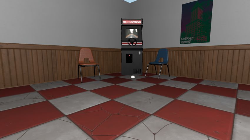
D. Lin & L. Seiler & C. Yuksel / Hardware Adaptive High-Order Interpolation for Real-Time Graphics
P01 D½1 P11 P01 D01 D11 P11 The standard bicubic interpolation with 16 control points ■C16
2D
can be written in a similar form by using the second derivatives,
D11 such that the desired second derivatives
D01 D01 D11 2
D0½ D1½t
∂ i+ j
P⃗i j⃗ = (−1)C (i, j)
2D
t (12)
D½½ D10 ∂s ∂t ■ 16
D00 D10
D00 are achieved using difference terms
2
i+ j∂
P00 D½0 P10 P00 D00 D10 P10 D⃗i j⃗ = P⃗i j⃗ − (−1) C (i, j)
2D
∂s ∂t □ 12
s s
= P⃗i j⃗ − (Pi j − P(1−i) j − Pi(1− j) + P(1−i)(1− j) ) (13)
(a) Biquadratic (b) Bicubic
− (D⃗i(1− j) − D⃗i j + D(1−i) j⃗ − Di j⃗) .
Figure 1: The difference terms of biquadratic and bicubic interpo- for i, j ∈ {0, 1}. With these internal difference terms, standard bicu-
lations in 2D. bic interpolation can be written as
■C16 (s,t) = □C12 (s,t)
2D 2D
(14)
2
3.2. 2D Interpolation + (1 − s)s(1 − t)t Lst (D0⃗0⃗ , D1⃗0⃗ , D0⃗1⃗ , D1⃗1⃗ ) .
In 2D, we rely on the bilinear interpolation operator In this form, standard bicubic interpolation involves an additional
2D
2 1 1 bilinear interpolation over □C12 .
Lst (P00 , P10 , P01 , P11 ) =(1 − t)Ls (P00 , P10 ) + tLs (P01 , P11 )
=(1 − s)(1 − t)P00 + s(1 − t)P10
3.3. 3D Interpolation
+ (1 − s)tP01 + stP11
This concept of representing higher-order interpolation as a sum of
Bilinear interpolation simply uses this operator, such that linear interpolation and higher-order terms can be extended to 3D
2 as well. In 3D, we can use the trilinear interpolation operator
(s,t) = Lst (P00 , P10 , P01 , P11 ) .
2D
■L4 (7)
3
Lstq (P000 , P100 , P010 , P110 , P001 , P101 ,P011 , P111 ) =
Biquadratic interpolation involves 9 control points: 4 at the ver- 2
tices, 4 at the edge centers, and one at the middle of the rectan- (1 − q) Lst (P000 , P100 , P010 , P110 )
2
gle they form (Figure 1a). Similar to the 1D case, we can write + q Lst (P001 , P101 , P011 , P111 )
biquadratic interpolation using difference values at the edge cen-
ters D½0 , D½1 , D0½ , D1½ , and the difference value at the middle This operator linearly blends two bilinear operators and trilinear
position D½½ . If we omit this middle difference value by taking interpolation simply uses it, such that
D½½ = 0, the resulting quadratic interpolation can be written as 3D 3
(s,t, q) = Lstq ( P000 , P100 , P010 , P110 ,
■L8 (15)
1
□Q8 (s,t) = ■L4 (s,t) + 4(1 − s)s Lt (D½0 , D½1 )
2D 2D
(8) P001 , P101 , P011 , P111 ) ,
1
+ 4(1 − t)t Ls (D0½ , D1½ ) . where Pi jk with i, j, k ∈ {0, 1} are the data values at the eight ver-
tices of a cube.
If the middle difference term D½½ is non-zero, biquadratic interpo-
lation becomes Again, for our quadratic and cubic interpolation functions, we
omit the higher-order difference terms inside the cube and on the
(s,t) = □Q8 (s,t) + 16(1 − s)s(1 − t)t D½½
2D 2D
■Q9 (9) face centers of the cube, resulting
and D½½ can be written using the desired middle value P½½ as
□Q20 (s,t, q) = ■L8 (s,t, q)
3D 3D
(16)
D½½ = P½½ − □Q8 (½, ½) .
2D
(10) 2
+ 4(1 − s)s Ltq ( D½00 , D½10 , D½01 , D½11 )
2
The standard bicubic interpolation involves 16 control points. + 4(1 − t)t Lsq ( D0½0 , D1½0 , D0½1 , D1½1 )
Similar to the quadratic case, if we omit the four difference terms in 2
+ 4(1 − q)q Lst ( D00½ , D10½ , D01½ , D11½ )
the interior of the rectangle and only consider the edges (Figure 1b),
we get
□C32 (s,t, q) = ■L8 (s,t, q)
3D 3D
(17)
□C12 (s,t) = ■L4 (s,t)
2D 2D
(11) + (1 − s)s
3
Lstq ( D0⃗00 , D1⃗00 , D0⃗10 , D1⃗10 ,
2
+ (1 − s)s Lst (D0⃗0 , D1⃗0 , D0⃗1 , D1⃗1 ) D0⃗01 , D1⃗01 , D0⃗11 , D1⃗11 )
2
+ (1 − t)t Lst (D00⃗ , D10⃗ , D01⃗ , D11⃗ ) . + (1 − t)t
3
Ltqs ( D00⃗0 , D01⃗0 , D00⃗1 , D01⃗1 ,
Note that, with this formulation, bicubic interpolation turns into D10⃗0 , D11⃗0 , D10⃗1 , D11⃗1 )
three linear interpolations: the first one interpolates the four vertex 3
+ (1 − q)q Lqst ( D000⃗ , D001⃗ , D100⃗ , D101⃗ ,
values and the other two interpolate the difference in the deriva-
tives. D010⃗ , D011⃗ , D110⃗ , D111⃗ ) .
© 2021 The Author(s)
Computer Graphics Forum © 2021 The Eurographics Association and John Wiley & Sons Ltd.
D. Lin & L. Seiler & C. Yuksel / Hardware Adaptive High-Order Interpolation for Real-Time Graphics
3D
Note that standard triquadratic and tricubic interpolations ■Q27 and
3D P-12 P02 P12 P22
■C64 use 27 and 64 control points, respectively. Therefore, the ver-
sions above that skip the interior difference terms save 7 and 32
control points for quadratic and cubic interpolation, respectively.
P-11 P01 P11 P21
t
3.4. Adaptive High-Order Interpolation P00 P10
P-10 P20
Notice that all our high-order interpolation formulations contain
high-order difference terms, i.e. D-terms, defined as the difference
between a quantity approximated by lower-order interpolation and P-1-1 P0 -1 P1-1 P2 -1
the desired value. These D-terms are indicators of how well linear
interpolation approximates the desire values. s
Figure 2: The texel data used for high-order filtering in 2D.
When the D-terms are close to zero, high-order interpolation pro-
duces results with relatively small difference from linear interpola-
tion. In such cases, simply using linear interpolation instead may be
an acceptable approximation. This opens up the possibility of adap-
tive high-order interpolation that skips the high-order difference In our formulation, the D⃗i j and Di j⃗ terms can be computed us-
terms when they are close to zero, determined by a user-defined 2D
ing Equation 19. These are sufficient for evaluating □C12 in Equa-
tion 14. For ■C16 we also need D⃗i j⃗ with i, j ∈ {0, 1}. They can be
threshold Dmin . 2D
At first glance, this may appear as a minor simplification, partic- computed using the desired second derivatives
ularly considering software interpolation. However, as we explain P(1−i) j + Pi(1− j) + Pi(3 j−1) + P(3i−1) j
in Section 4, adaptive interpolation can be used for more than dou- D⃗i j⃗ = Pi j − (21)
2
bling the throughput of a hardware implementation. P(1−i)(1− j) + P(3i−1)(1− j) + P(1−i)(3 j−1) + P(3i−1)(3 j−1)
+
4
3.5. High-Order Texture Filtering 2D
Note that computing these last four D-terms for ■C16 involves com-
Bicubic image filtering is known to produce superior image quality, bining 9 data points Pi j within a 3 × 3 block.
as compared to bilinear, and it is often used for enlarging raster
images. Using a Catmull-Rom spline, interpolation along 1D can Quadratic interpolation for texture filtering is not as popular.
be written as This is because it involves accessing the same amount of texture
1 2
data as cubic interpolation and it cannot deliver the same quality.
Ss (P-1 , P0 , P1 , P2 ) = − s(1 − s) /2 P-1 Nonetheless, it is still superior to linear filtering and requires less
3 2 2
+ ((1 − s) + 3s(1 − s) + s (1 − s)/2) P0 computation than cubic. Therefore, it might be preferable for some
applications.
3 2 2
+ (s + 3s (1 − s) + s(1 − s) /2) P1
We define quadratic interpolation similarly, using Catmull-Rom
2
− s (1 − s)/2 P2 splines. In this case, the D-terms ensure that the interpolation
matches the Catmull-Rom spline at the middle points. Thus, in 1D
1D cubic interpolation can simply use this function
we can write
1
(s) = Ss (P-1 , P0 , P1 , P2 ) .
1D
■C4 (18) −P-1 + P0 + P1 − P2
D½ = . (22)
For our cubic interpolation, however, we must first compute the 16
D-terms. Using a Catmull-Rom spline (with uniform parameteri- 2D
In 2D, we can compute the D-terms for □Q8 similarly. As for
zation) that interpolates the data points P−1 , P0 , P1 , and P2 , the 2D
■Q9 , the computation of the middle difference term involves all
D-terms can be written as
16 data points, using
Pi−1 + Pi+1
D⃗i = Pi − (19)
D½½ = ■C16 (½, ½) − □Q8 (½, ½) .
2D 2D
2 (23)
for i ∈ {0, 1}. Then, we can use our ■C4 formulation in Equation 6.
1D
Note that in both biquadratic and bicubic interpolations, evaluat-
Similarly, bicubic interpolation using a 4 × 4 block of texel sam- 2D 2D
ing the D-terms for □Q8 and □C12 are much simpler than the ad-
ples shown in Figure 2 can be defined using Catmull-Rom splines, 2D 2D 2D 2D
ditional D-terms needed for ■Q9 and ■C16 . Also, □Q8 and □C12
such that
do not need to access the corner texels P-1-1 , P2-1 , P-12 , and P22 .
1 1
■C16 (s,t) = Ss ( St ( P-1-1 , P-10 , P-11 , P-12 ),
2D
(20) These corner texels are only needed for computing the internal D-
2D 2D
1 terms used by ■Q9 and ■C16 .
St ( P0-1 , P00 , P01 , P02 ),
1 The equations for triquadratic and tricubic cases are similar.
St ( P1-1 , P10 , P11 , P12 ), 3D 3D
1
Again, the D-terms for □Q20 and □C32 are much simpler to com-
St ( P2-1 , P20 , P21 , P22 ) ) . 3D 3D
pute than ■Q27 and ■C64 .
© 2021 The Author(s)
Computer Graphics Forum © 2021 The Eurographics Association and John Wiley & Sons Ltd.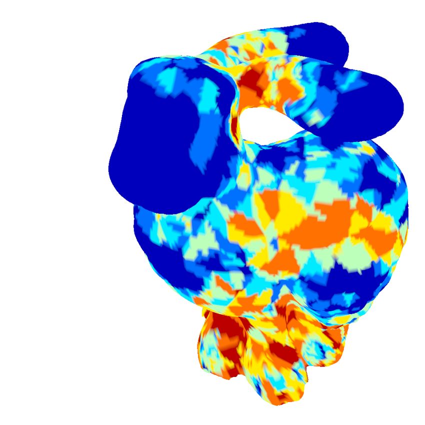
D. Lin & L. Seiler & C. Yuksel / Hardware Adaptive High-Order Interpolation for Real-Time Graphics

4. High-Order Hardware Texture Filtering                                       4.2. Current Texture Cache Access Methods
The versions for quadratic and cubic interpolations we present in              Texture units in GPUs are fed by deep queues of pending filter op-
Section 3 provide convenient mechanisms for hardware implemen-                 erations. This provides time to compute filter weights, determine
tation. In this section, we discuss the details of existing GPU texture        which texels will be accessed, and load the texels into caches. Typ-
filtering hardware and how it can be modified to support high-order            ically there are multiple cache levels, e.g. a large cache shared over
interpolation using our formulations.                                          the whole GPU that feeds L2 and specialized L1 caches that are
                                                                               dedicated to individual texture units. The operation queue is typi-
                                                                               cally sized to cover the latency of accessing off-chip memory, so
4.1. Texture Filtering on Current GPUs                                         that BOPs can usually occur without off-chip memory read delays.
Bilinear interpolation is a fundamental texture filtering operation               The L1 caches in texture units are specialized to allow a BOP
on the GPU. Current GPUs implement it in one of two ways                       per cycle without cache read delays. Bilinear texture filtering re-
[MSY19]. The first way is to linearly interpolate pairs of texels              quires accessing an unaligned 2 × 2 of texels. For a standard cache
along one dimension, then linearly interpolate the results along the           or memory this could require 1, 2, or 4 memory accesses, depend-
other dimension, using 3 linear interpolations. The second way is              ing on how the unaligned 2 × 2 block maps onto the aligned blocks
to compute a weight for each of the four texels, then multiply them            that are stored in cache or memory. This is not a problem when
and add the four results. This requires an extra multiplier but al-            reading texels from memory or from the L2 cache, since nearby
lows more parallelism. It also requires only one renormalization               texel values are likely to be used in later texture filter operations.
for floating point textures instead of three. Our adaptive higher or-          But requiring multiple read cycles from the L1 cache has obvious
der interpolation method works with both of these implementation               problems for maintaining the desired texture processing rate of one
methods.                                                                       BOP per clock.
   Texture units in GPUs perform certain filtering operations in                  The standard solution is to divide the L1 texture cache into four
multiple steps. For example, trilinear filtering uses two bilinear op-         banks, based on the low order bits of the U and V indices of the
erations. The result of each bilinear operation, or BOP for short, is          stored texture coordinates. The left side of Figure 3 illustrates how
scaled and accumulated to produce the trilinear result. This is il-            this works: texels are stored in banks based on whether their U and
lustrated in Figure 3. Alternately, the GPU could perform the two              V indices are even or odd. Texture dimensions are padded to some
BOPs in parallel, linearly interpolating the pair of results. The area         tile size, typically at least 4 texels, so for each texture, one quarter
involved is similar and the former method allows pure bilinear fil-            of its texels fall into each of the four buffers. As a result, a bilinear
tering operations to go twice as fast, while supporting two two-step           interpolation unit can receive an unaligned 2 × 2 of texels on each
trilinear operations in parallel, so the raw throughput of trilinear           clock by computing the appropriate memory addresses for each of
operations is the same. Therefore, we will assume that the GPU im-             the four banks of texture L1 cache.
plements BOPs, although our method can also be adapted to work
with a GPU designed with trilinear filtering as the basic operation.              Finally, the number of L1 cache banks used depends on the num-
                                                                               ber of texels that must be accessed in parallel. For example, GPUs
                                                                               that perform a trilinear filter in a single clock cycle require eight
                                                                               banks. Four of the banks provide an unaligned 2 × 2 access for even
                                                                               mip levels or even slice numbers. The other four banks provide an
                                                                               unaligned 2 × 2 access for odd mip levels or odd slice numbers.

                                                                               4.3. High-Order Texture Filtering on Hardware
                                                                               High-order filtering with our formulations begins with linear inter-
                                                                                                  2D              3D
                                                                               polation (using ■L4 in 2D and ■L8 in 3D). This is exactly what
                                                                               the current hardware is designed to do. Then, we add the D-terms.
Figure 3: Texture filter unit on current GPUs. Bilinear operations             Notice that with all our quadratic and cubic formulations, except
(BOPs) can be scaled and accumulted to perform more complex                            2D
                                                                               for ■Q9 , the D-terms can be processed in groups of 4. The com-
filtering. The L1 texture cache is divided into four interleaved banks         putation of each group is the same as a BOP multiplied by a scale
to allow parallel access to an unaligned 2×2 of texels.                        factor.
                                                                                   Computing the scale factors (e.g. (1 − s)s, (1 − t)t, etc.) needed
   Another multi-step texture filtering operation is anisotropic fil-
                                                                               for the steps involving the D-terms can be pipelined, so they do not
tering. In this case, up to 16 individual bilinear or trilinear filter re-
                                                                               require extra clock cycles. The amount of additional logic required
sults are blended to approximate an elongated filter region. There-
                                                                               is relatively small as well. For example, with 8-bit precision (1−s)s
fore, even if a texture unit implements trilinear filtering as its basic
                                                                               can be computed with an 8 × 8 multiplier, though we used 32-bit
operation, it still needs to scale and accumulate the results of mul-
                                                                               floating point numbers for tests in Section 7.
tiple BOPs to support anisotropic filtering. Since the number of
BOPs is the bottleneck for computation, we use that to represent                  Computing the D-terms is also straightforward, given access to
the computational cost of our texture interpolation techniques.                the necessary texels. Figure 4 shows that the D-term calculation is

                                                                                                                                                    © 2021 The Author(s)
                                                                                  Computer Graphics Forum © 2021 The Eurographics Association and John Wiley & Sons Ltd.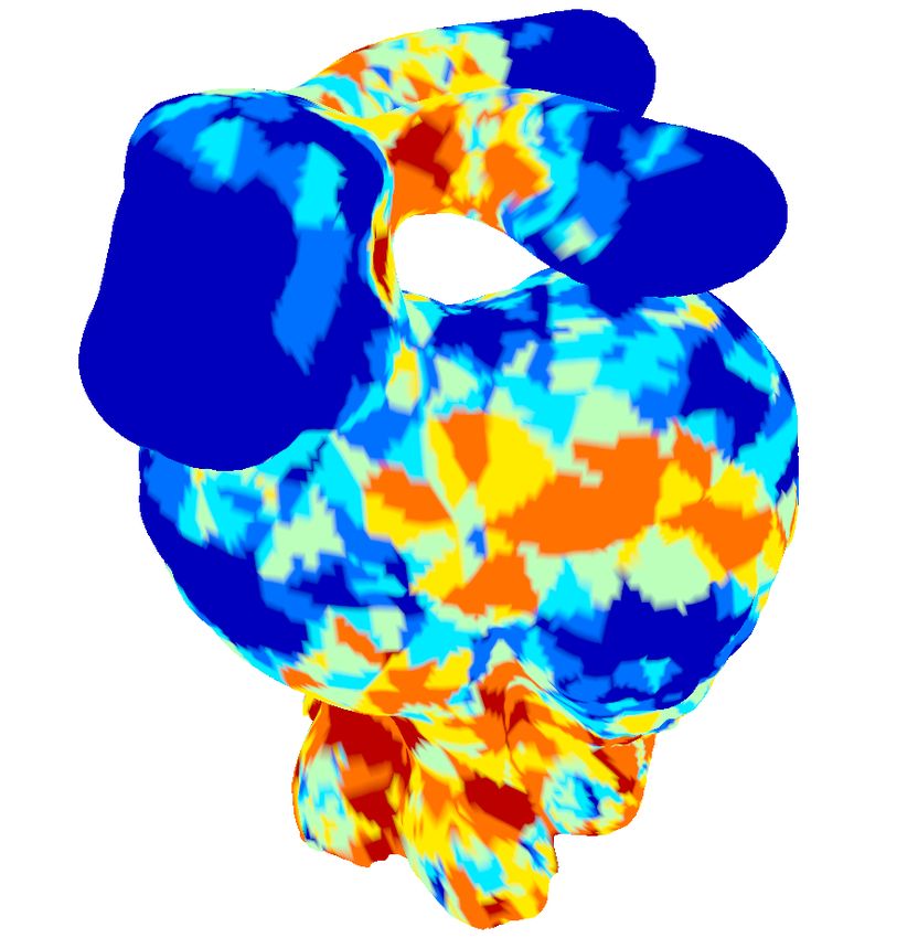
D. Lin & L. Seiler & C. Yuksel / Hardware Adaptive High-Order Interpolation for Real-Time Graphics

                                                                                         since the filter kernels near neighboring texels largely overlap.
                                                                                         Therefore, we can expect the higher level caches to efficiently han-
                                                                                         dle the data flow. However, the L1 cache must be changed to allow
                                                                                         accessing more texels in parallel.
                                                                                            As illustrated in Figure 4, using more banks in the L1 cache
                                                                                         allows computing the D-terms in parallel to achieve peak perfor-
                                                                                         mance. Then, groups of 4 D-terms can be passed to the existing
                                                                                         bilinear interpolation logic. The L1 cache can be implemented us-
                                                                                         ing 4, 8, 16, or 32 banks with different levels of performance, as we
Figure 4: Proposed texture filter unit for higher order interpola-                       discuss in Appendix A.
tion. The L1 texture cache is divided into 4, 8, 16, or 32 interleaved
banks to allow parallel access.
                                                                                         5. Extensions to Interpolation in Simplexes
                                                                                         In Section 3 we described our difference-based formulations of
pipelined between the texel L1 cache read and the bilinear opera-                        quadratic and cubic interpolations for structured sample data in a
tion. Therefore, utilizing the existing BOP logic unit, we can in-                       grid. In this section, we extend this concept to arbitrary simplexes,
clude the D-terms for high-order filtering by simply using the same                      such as line segments (1D), triangles (2D), and tetrahedra (3D).
unit multiple times. This way, high-order filtering simply involves                      Similar to our notation for grids, (cubic) interpolations are repre-
                                                                                                        nD                                  nD
additional steps, similar to computing trilinear filtering with two                      sented as △Cm , if they omit some terms, and ▲Cm , if they include
bilinear filtering steps or anisotropic filtering in multiple steps on                   all terms, where n is the dimension and m is the total number of
current hardware.                                                                        interpolated data values, including the simplex vertices.
   The cost of computing the D-terms depends on the filtering op-
eration being performed. Computing the D-terms along the edges                           5.1. Interpolation in a Simplex
                                                      2D     2D     3D
needed for quadratic and cubic interpolations □Q8 , □C12 , □Q20 ,
          3D
and □C32 , only require adders and bit-shifters (for division by a                       A simplex in n-dimensions is defined by n + 1 vertices. Let Pi
power of 2), which do not require much extra area or power. The                          where i ∈ {0, . . . , n} represent the data values at the vertices and
                                                                                                               T
                                                              2D
internal D-terms for quadratic and cubic interpolations ■Q9 , ■C16 ,
                                                                    2D                   w = [w0 , . . . , wn ] is the barycentric coordinates of the interpola-
    3D            3D                                                                     tion point, forming a partition of unity, such that
■Q27 , and ■C64 involve more expensive operations to evaluate
from the data points P, so they require a greater area cost when                                                        n
modifying existing texture filtering hardware. Based on the num-                                                        ∑ wi = 1 .                            (24)
                                         2D                  2D                                                         i=0
ber of D-terms, we can process □Q8 with 2 BOPs, □C12 with 3
             3D                        3D
BOPs, □Q20 with 5 BOPs, and □C32 with 8 BOPs in total. The in-                           Linear interpolation is defined as a simple weighted average, using
                                                             2D     2D
terpolations that involve the internal D-terms, such as ■Q9 , ■C16 ,                                                              n
    3D           3D
                                                                                                                ▲Ln+1 (w) = ∑ wi Pi
  Q    , and   C    , would require 3, 4, 6, and 16 BOPs, respectively.                                            nD
■ 27          ■ 64                                                                                                                          .                 (25)
                                                                                                                            i=0
   These numbers imply a dramatic reduction of performance com-
pared to bilinear interpolation, but we can improve performance
by using adaptive high-order interpolation, as we discussed in Sec-                                        P2                                     P2
tion 3.4. Computation of the D-terms is pipelined in advance of per-
forming BOPs, so adaptive filtering can be implemented by check-
                                                                                                                                      D02              D23
ing the four D-terms to be used for the next step. If they all are
                                                                                              D02                 D12
below the given threshold Dmin , the bilinear step can be skipped. If                                                                           D12
all of the D-terms are below the threshold, higher order interpola-
                                                                                                                                                             P3
tion requires just 1 BOP and so has the same performance as linear                                                               P0                      D13
interpolation.                                                                                                                              D01
    For high-order interpolation involving more than 2 steps, instead                    P0             D01                 P1                          P1
of using pre-defined groups of D-terms, it is possible to group the                      Figure 5: The high-order difference terms for quadratic interpola-
D-terms that pass the threshold for minimizing the number of steps.                      tion on a triangle and in a tetrahedron.
However, this would require more complex logic, so we assume
pre-defined groups of D-terms in our evaluation (Section 7). Still,                         For quadratic interpolation, we define high-order difference
it is possible to save power by simply turning off the multiplier for                    terms Di j between each pair of vertices i and j with i < j, as shown
any D-term that is below the threshold.                                                  in Figure 5. Then, quadratic interpolation can be written as
                                                                                                                                      n−1   n
                                                                                            ▲Q(n+1)(n+2)/2 (w) = ▲Ln+1 (w) + ∑ ∑ 4 wi w j Di j
                                                                                               nD                       nD
4.4. Texture Cache Access for Higher Order Filtering                                                                                                     .    (26)
                                                                                                                             i=0 j=i+1
High-order texture interpolation involves accessing more data, but
this does not necessarily inflate the off-chip memory bandwidth,                         There are n(n + 1)/2 quadratic D-terms: a line has 1, a triangle

© 2021 The Author(s)
Computer Graphics Forum © 2021 The Eurographics Association and John Wiley & Sons Ltd.
D. Lin & L. Seiler & C. Yuksel / Hardware Adaptive High-Order Interpolation for Real-Time Graphics
P2 P2 smooth normals for shading a triangle, the D-terms can be com-
D20 D23 puted on-the-fly from the triangle’s vertex positions and normals
D20 D21 [VPBM01]. Also, the D-terms can be computed on-the-fly for
D02 D21 D32 barycentric filtering using mesh color textures [Yuk17] or patch
textures [MSY19] for providing hardware texture filtering support
D02 D12 D012 P3
D12 for mesh colors [YKH10], as they use structured triangular texel
D012 P0 distributions.
D01
D10 Another example is a regular simplex mesh in a grid, such as
P0 D01 D10 P1 P1 a triangular mesh or a tetrahedral mesh with vertices on a regular
Figure 6: The high-order difference terms for cubic interpolation grid. A 2D grid cell can be represented using two triangles and
on a triangle and in a tetrahedron. a 3D grid cell can be formed by 5 or 6 tetrahedra. Indeed, the
vertex data for such meshes can be stored in 2D or 3D textures.
This offers a cheaper alternative to texture filtering using fewer data
2D 3D points, and it can be used for applications like color space conver-
has 3, and a tetrahedron has 6. Thus, we get ▲Q6 and ▲Q10 for
sion [KNPH95] that can benefit from high-order filtering.
triangles and tetrahedra, respectively.
When the D-terms cannot be computed during interpolation and
For defining cubic interpolation, we use Di⃗j to specify the de-
must be pre-computed, adaptively skipping some D-terms can pro-
sired derivatives along each edge, as shown in Figure 6. Then, we
vide storage, memory bandwidth, and computation savings at run
can write our cubic interpolation formulation as
time.
△C(n+1)2 (w) = ▲Ln+1 (w)
nD nD
(27)
n−1 n 6. Hardware Interpolation for Simplex Meshes
+ ∑ ∑ wi w j (wi Di⃗j + w j D ⃗ji ) .
i=0 j=i+1
For providing hardware-accelerated interpolation, there are two
cases to consider: regular simplex meshes on a grid and arbitrary
2D 3D
This formulation defines △C9 and △C16 for triangles and tetrahe- simplex meshes.
dra, respectively, only considering the derivatives along the edges
The data for regular meshes of triangles or tetrahedra can be
of the simplex. For triangles, however, cubic interpolation can also
stored in 2D or 3D grids. In that case, hardware interpolation can
specify a desired value P012 at the center using an interior dif-
be supported in a similar way as described in Section 4. The only
ference term D012 = P012 − △C9 (wcenter ), where wcenter = 1/3 is
2D
differences are the interpolation functions and the subsets of the
the barycentric coordinates of the center of the triangle. Including
texel data blocks used in the interpolation (Section 6.1).
higher-dimensional simplexes, we can write
Arbitrary simplex meshes, however, cannot be handled similarly
▲C(n+1)(n2 +1) (w) = △C(n+1)2 (w)
nD nD
(28)
and require a different treatment (Section 6.2).
n−2 n−1 n
+∑ ∑ ∑ 27 wi w j wk Di jk .
i=0 j=i+1 k= j+1 6.1. Hardware Interpolation for Regular Simplexes
i jk i jk For regular triangles on a grid, the existing bilinear interpolation
Here, Di jk = Pi jk − △C(n+1)2 (wcenter ), where wcenter is the
nD
unit can be modified to support barycentric linear interpolation
barycentric coordinates for the center of the triangle formed by
012 [MSY19]. One of the four texels is weighted as zero and the other
verices i, j, k of the simplex (e.g. for a tetrahedron, wcenter = three use weights that produce the same result as barycentric inter-
T
[ /3 /3 /3 0] ).
1 1 1
polation. This can be done for both methods of designing the bilin-
Note that this formulation provides n(n − 1)(n + 1)/6 interior ear operation block, that is using three linear interpolation units or
D-terms: a triangle has 1 and a tetrahedron has 4. The resulting using four parallel multipliers.
2D 3D
interpolations for triangles and tetrahedra are ▲C10 and ▲C20 , re- Our method for supporting nonlinear triangular interpolation ex-
spectively. tends this method. Reading an unaligned 4 × 4 array of texels al-
lows D-terms to be computed. These are then fed into the bilinear
operation block, along with appropriate weights. In general, up to
5.2. Practical Interpolation Applications Using Simplexes
three D-terms can be retired per cycle through the bilinear opera-
High-order interpolations within a grid described in Section 3 al- tion logic.
low computing the D-terms from the data points on-the-fly. In the
A similar method may be used for regular tetrahedra in a 3D grid.
case of arbitrary simplex meshes, however, a typical application-
Linear interpolation can be achieved with an unaligned 2 × 2 × 2
needs to pre-compute the D-terms. This is because determining the
array of texels. Four of the texel values are used and the rest are
desired derivatives or the edge/triangle center values typically re-
ignored. The four chosen vertices are gathered into a single BOP. If
quires traversing the simplex topology, using discrete differential
the BOP is implemented using four multipliers, these get the four
geometry operators [MDSB03].
barycentric parameters. If the BOP is implemented using three lin-
There are exception, however. For example, reconstructing ear interpolations, the weights for the first pair are w0 /(w0 + w1 )
© 2021 The Author(s)
Computer Graphics Forum © 2021 The Eurographics Association and John Wiley & Sons Ltd.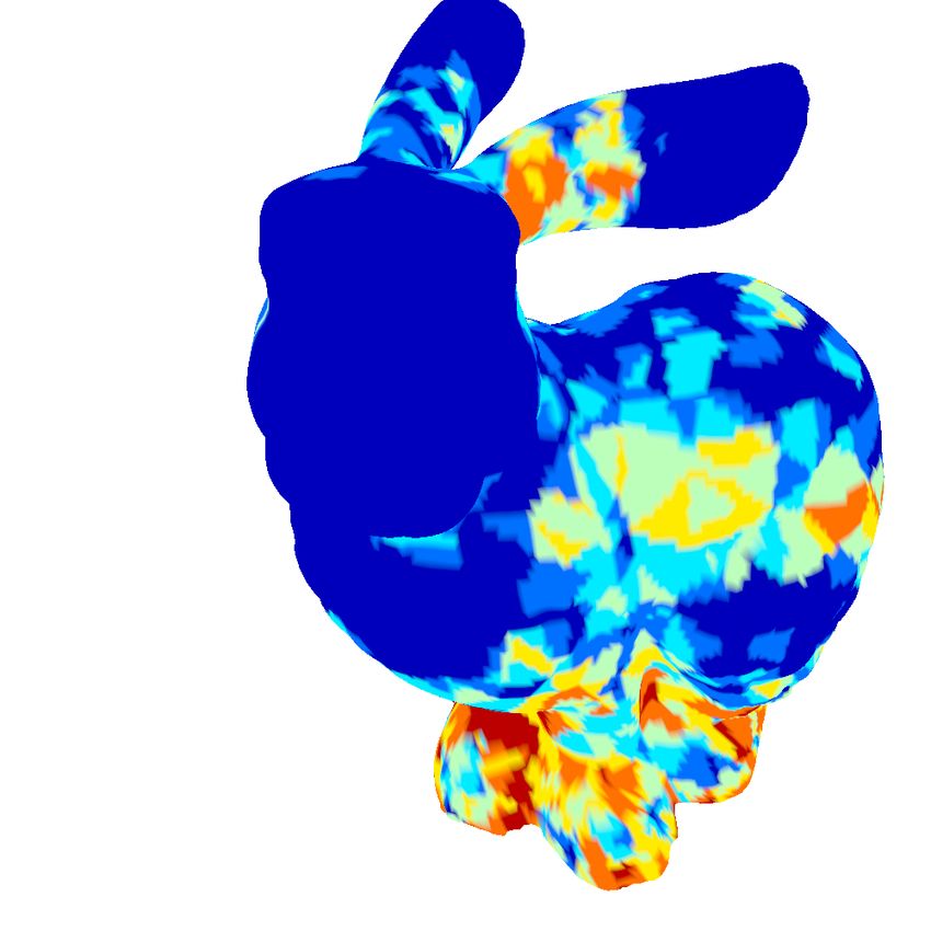
D. Lin & L. Seiler & C. Yuksel / Hardware Adaptive High-Order Interpolation for Real-Time Graphics
                                                2D                                    2D                            2D                              2D
              Reference                       □C12 ,   Ratio of ∣D∣ ≥ 0.048         □C12 ,   Ratio of ∣D∣ ≥ 0.2   □Q8 ,   Ratio of ∣D∣ ≥ 0.0095   □Q8 ,   Ratio of ∣D∣ ≥ 0.0315
                        2   2
     240(cos(0.0008(x + y )) + 1)                      (25% clamped)                         (50% clamped)                 (25% clamped)                   (50% clamped)

                  (a)                                       (b)                                  (c)                           (d)                             (e)
Figure 7: We test with a sinusoidal function (the image spans a parameter range from (0, 0) to (1, 1)). The reference image (left) is sampled
using 1024 × 1024 resolution (the compared insets are highlighted), while our tested methods upsample a 128 × 128 resolution input to
1024 × 1024 resolution. We visualize the ratio of D-terms in bicubic interpolation that are above a threshold (middle and right). Dark red
stands for 1 (all 8 D-terms for the pixel are above the threshold), and dark blue stands for 0.

and w2 /(w2 + w3 ). The weight for the linear interpolation that                                    cuboidal cases. In each application, we compare the quality of our
combines them is (w0 + w1 )/(w0 + w1 + w2 + w3 ).                                                   result to linear interpolation. We show how our result achieves sim-
                                                                                                    ilar quality as non-adaptive high-order interpolation by only com-
   Our method for supporting nonlinear tetrahedral interpolation
                                                                                                    puting high-order interpolation when necessary. By exploiting the
extends this method. All D-terms to be computed using an un-
                                                                                                    sparseness of high-frequency information, our method can discard
aligned 4 × 4 × 4 array of texels. They are then fed into the bilinear
                                                                                                    most high-order terms in many applications, making it run at a com-
operation block as barycentric operations, along with appropriate
                                                                                                    parative performance or use similar amount of storage as linear in-
weights. In general, up to four D-terms can be retired per cycle
                                                                                                    terpolation. We also compare with the state-of-art high-order inter-
through the bilinear operation logic.
                                                                                                    polation method for the application, if one exists and show how our
                                                                                                    method improves the performance while delivering similar quality.
6.2. Hardware Interpolation for Arbitrary Simplexes                                                   For interpolations in grids, we use the number of BOPs com-
Linear barycentric interpolation for triangles can be performed ei-                                 puted as the performance metric for comparing different methods.
ther in hardware or using code attached to the start of the fragment                                For simplex mesh examples targetting software implementation,
shader. Either way, it typically supports multiplying three barycen-                                we report shader execution times on current hardware.
tric coefficients times three parameter values.
   D-terms for quadratic and cubic triangular interpolation can be                                  7.1. 2D Texture Filtering
generated e.g. in a geometry shader and then passed to the frag-                                    First, we present results using a synthetic texture that contains
ment shader. The interpolation can be performed using either logic                                  a variety of frequencies, shown in Figure 7. Given a threshold
                                                                                                                                               2D
or shader code that computes products of the barycentric terms and                                  Dmin = 0.048 for bicubic interpolation □C12 , 25% of the D-terms
multiplies them in turn by the D-terms. In hardware this could be                                   are eliminated (Figure 7b-c). The higher frequency region shows
performed using multiple passes through the existing logic, elim-                                   higher ratio of D-terms with magnitude greater than the threshold.
inating the extra hardware multiplies where the D-terms are zero.                                   Below a certain frequency, all D-terms are below the threshold. Us-
Typically, GPU shader instructions support testing conditionals in                                  ing Dmin = 0.2, 50% of the D-terms are clamped. The observation
                                                                                                                                                2D
parallel with ALU operations, so testing to see if D-terms can be                                   is similar for biquadratic interpolation □Q8 (Figure 7d-e). With
eliminated does not need to reduce the performance of a shader                                      Dmin = 0 we turn off clamping and all D-terms are used.
code implementation, either.
                                                                                                       A comparison between different interpolation methods using
   Tetrahedral interpolation is performed in the same way, except                                   parts of the same synthetic texture can be found in Figure 8. Our
                                                                                                                             2D
with four barycentric terms instead of three. This is not needed in                                 bicubic interpolation □C12 with Dmin = 0 generates almost identical
                                                                                                                                                2D
pixel shaders, but can be useful in vertex shaders (as illustrated                                  result as standard bicubic interpolation ■C16 . This shows that the
in Section 7.5) as well as geometry shaders. As for the software                                    impact of omitting the 5th and 6th order terms is relatively minor
implementation of unstructured triangles, shader code computes D-                                   in this example. When increasing Dmin to 0.048 to clamp 25% of
terms for unstructured tetrahedra and then performs the necessary                                   the D-terms, the difference is hard to notice. With Dmin = 0.2, the
multiplies and adds for non-zero sets of D-terms.                                                   low-frequency inset begins to show patterns related to bilinear in-
                                                                                                    terpolation, because most D-terms are clamped. However, the high-
                                                                                                    frequency inset still looks unchanged, because higher-frequency
7. Evaluation                                                                                                                                                     2D
                                                                                                    regions contain more pixels with larger D-terms. Our □Q8 bi-
We demonstrate the effectiveness of our hardware adaptive high-                                     quadratic interpolation also produces almost identical result as the
                                                                                                                        2D
order interpolation method in 5 different real-time rendering ap-                                   more expensive ■Q9 version. Dmin affects the results similarly to
plications to cover all of rectangular, triangular, tetrahedral, and                                the bicubic case.

© 2021 The Author(s)
Computer Graphics Forum © 2021 The Eurographics Association and John Wiley & Sons Ltd.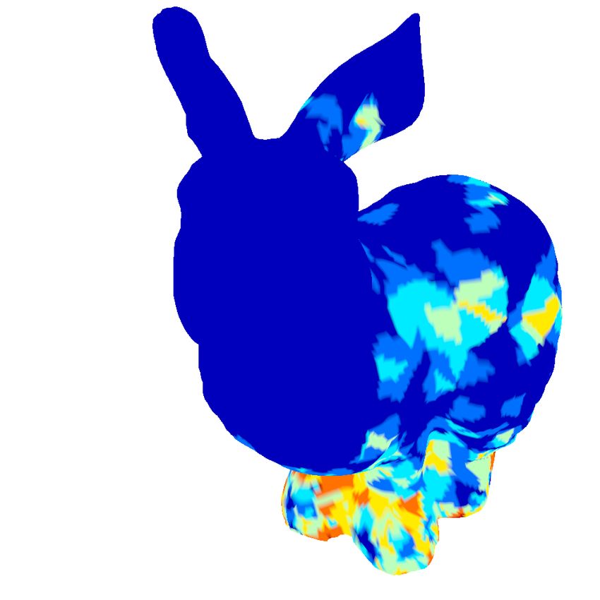
D. Lin & L. Seiler & C. Yuksel / Hardware Adaptive High-Order Interpolation for Real-Time Graphics

                                                      Our Bicubic Interpolation                                                        Our Biquadratic Interpolation
                               2D                2D            2D              2D                           2D                               2D          2D               2D
       Reference          ■C16                 □C12        □C12 (-25%D)      □C12 (-50%D)    ■Q9                                           □Q8         □Q8    (-25%D)   □Q8    (-50%D)         Bilinear
                    (Standard Bicubic)      No Clamp          Dmin = 0.048     Dmin = 0.2   No Clamp                                      No Clamp      Dmin = 0.0095    Dmin = 0.0315
 MSE: 0 (reference)      0.01304             0.01362           0.01365          0.01408      0.01413                                       0.01458        0.01462          0.01520             0.02429

Figure 8: A comparison of different interpolation method for upsampling the sinusoidal function from 128 × 128 to 1024 × 1024. The first
and third row: insets. The second and fourth row: 4 × and 1 × difference images with respect to the reference.

    0.024
                                                                                              Bilinear operations per pixel

                                                                                                                              5
                    Bilinear                                                                                                                                                      [Csébfalvi 2018]
    0.022
                         (Bicubic)                                                                                            4                                                          (Bicubic)
       0.02                                                                                                                                                                             Ideal Case
                         (Biquadratic)
                                                                                                                              3                                                        (Biquadratic)
                    Standard Bicubic
 MSE

    0.018                                                                                                                                                                         Bilinear

                                                                                                                              2
    0.016

                                                                                                                              1
    0.014

    0.012                                                                                                                     0
              0%        20%              40%            60%          80%          100%                                            0%           20%          40%          60%             80%           100%
                               Percentage of clamped                                                                                                 Percentage of clamped

Figure 9: Comparing MSE of different interpolation method using                             Figure 10: Comparing average bilinear operations per pixel of dif-
different Dmin (only our bicubic and biquadratic interpolation is                           ferent methods for the sinusoidal function upsampling.
affected) for the sinusoidal function upsampling.

                                                                                            texture is modified by modulating the input texture with a check-
   In Figure 9, we compare mean square error (MSE) of differ-
                                                                                            board pattern of 1 and −1 values.
ent interpolation methods. With Dmin = 0, our bicubic interpola-
        2D
tion □C12 produces a slightly higher MSE than the standard bicu-                               In Figure 10, we visualize the average BOPs per pixel for each
                     2D
bic interpolation ■C16 , due to the omission of 5th and 6th or-                             method. We see that even using Dmin = 0, our bicubic interpolation
                                           2D
der terms. Our biquadratic interpolation □Q8 produces a slightly                            (3 per pixel) has fewer number of BOPs than Csébfalvi’s method
higher MSE. Nonetheless, MSE for all high-order interpolations is                           (5 per pixel). Using adaptive higher-order filtering with Dmin > 0,
                                                                                                                                                             2D
much lower than bilinear. As expected, MSE grows with increasing                            we can improve the performance further. The solid line for □C12
Dmin .                                                                                      shows the performance when groups of 4 D-terms are formed in a
                                                                                            predefined order and a BOP is skipped only when all D-terms in a
   We compare the performance of our approach to Csébfalvi’s
                                                                                            group are below the threshold. The dashed line shows the ideal case
method [Csé18], the most efficient implementation of standard
                                                                                            that dynamically groups the D-terms for maximum performance.
bicubic interpolation on current GPU hardware. This method uses
                                                                                            Our biquadratic interpolation starts at a cheaper cost of 2 BOPs at
5 bilinear operations (4 bilinear texture access on the GPU plus 1
                                                                                            Dmin = 0 and decreases slowly with increasing Dmin .
bilinear operation for combining 4 terms with weights) to produce
the same result as standard Catmull-Rom bicubic interpolation. The                            To see how our bicubic rectangular interpolation works in prac-

                                                                                                                                                                     © 2021 The Author(s)
                                                                                                   Computer Graphics Forum © 2021 The Eurographics Association and John Wiley & Sons Ltd.
D. Lin & L. Seiler & C. Yuksel / Hardware Adaptive High-Order Interpolation for Real-Time Graphics
2D No TAA TAA TAA 64×
Our Bicubic Interpolation (□C12 ) Dmin = 0.2 bilinear operation heatmap TAA (bilinear lookup) (bicubic, adaptive) (bicubic lookup) Supersampling
2D 2D
Bilinear □C12 , Dmin = 0.2 □C12 , No Clamp Standard Bicubic
−4 −4 −6
MSE: 6.9 × 10 MSE: 1.6 × 10 MSE: 4.6 × 10 MSE: 0 (reference)
BOPs/read: 1 BOPs/read: 1.57 BOPs/read: 3 BOPs/read: 5
Figure 12: A comparison of 3 different history buffer lookup meth-
ods. Note that jagged edges can be seen when not using TAA. A ren-
dering using 64× supersampling is provided as the ground truth.
Note that bicubic lookup avoids the blurring of object edges and
texture details in as can be seen in result using bilinear lookup.
Bicubic adaptive lookup using Dmin = 0.003 produces highly simi-
lar result to using no clamping.
is due to reprojected positions landing at fractional pixel locations,
which requires interpolation to gather colors from nearby pixels.
As can be seen in Figure 12, using bicubic interpolation reduces
resampling blur as compared to bilinear interpolation.
Using our method with hardware modification, it is possible to
bring down the cost of bicubic interpolation to a level close to bi-
linear interpolation, while preserving most of the quality, as shown
2D
in Figure 13. Without clamping, our □C12 brings down the BOPs
per pixel to 3 to produce visually identical results standard bicubic
interpolation. Using Dmin = 0.003, more than 80% of bilinear op-
erations related to higher-order terms can be skipped. The result is
Figure 11: Comparing texture magnification filtering quality of bi- that only 39% more bilinear operations than pure bilinear interpola-
linear interpolation and our bicubic interpolation with no clamp- tion are executed to achieve a result almost identical to full bicubic
ing and adaptive clamping with Dmin = 0.2. A bilinear operation interpolation. The bilinear operation heatmap in Figure 13 shows
heatmap at Dmin = 0.2 is provided (Red: 3 bops, Yellow: 2 bops, that these discarded bilinear operations are mainly in regions with
Blue: 1 bop). Third and fifth row: 4× difference images with respect slowly varying color, while bicubic interpolation are preserved at
to standard bicubic interpolation of the insets in the rows above. high frequency regions like object edges and texture gradient edges,
which suffers more from resampling blur. Even though these results
use many state-of-art TAA improvement techniques provided by
tice, we test the texture filtering quality in the San Miguel scene, the Falcor engine [Kar14], including neighborhood clamping and
2D
shown in Figure 11. We observe that our □C12 produces indis- adaptive blending, they are insufficient for removing the resam-
2D
tinguishable result to standard bicubic interpolation ■C16 . Setting pling blur caused by bilinear interpolation. Bicubic interpolation,
Dmin = 0.2 produces visually very similar result with only 1.57 however, visibly improves the results.
BOPs on average, in contrast to 3 BOPs without clamping, and 5
BOPs with Csébfalvi’s method [Csé18] for standard bicubic inter-
polation. 7.3. Volume Rendering
We use volume rendering as an application to test our tricubic in-
3D
7.2. Temporal Anti-aliasing terpolation □C32 . Our test scene contains a volumetric teapot with
isotropic scattering and a directional light shown in Figure 14. The
Another use case of bicubic interpolation is temporal anti-aliasing
density data of the volume is defined in a 3D grid. We use ray
(TAA). TAA is widely used in today’s game engines. It reuses sub-
marching to compute the radiance reaching the camera. At each
pixel samples accumulated in previous frames to achieve the ef-
ray marching step, a density value is queried for computing the ex-
fect of supersampling. This is done by jittering the camera to cover
tinction coefficient. The lighting is gathered from a directional light
many sample positions in each pixel across several frames. When
with the visibility along the shadow ray computed via ray march-
the camera or the scene objects are moving, motion vectors need to
ing. We compare our performance to Csébfalvi’s tricubic volume
be calculated to fetch the pixel that corresponds to the same shading
density filtering method [Csé19]. Note that the Csébfalvi’s method
point in the history buffer (i.e. reprojection).
uses 7 trilinear taps on the current hardware, which is equivalent
One problem of TAA is known as resampling blur [YLS20]. This to 14 bilinear operations. In comparison, our method only uses 8
© 2021 The Author(s)
Computer Graphics Forum © 2021 The Eurographics Association and John Wiley & Sons Ltd.D. Lin & L. Seiler & C. Yuksel / Hardware Adaptive High-Order Interpolation for Real-Time Graphics
2D 3D
Our Bicubic Interpolation (□C12 ) Dmin = 0.003 bilinear operation heatmap Our Tricubic Interpolation (□C32 ) Dmin = 0.01 bilinear operation heat map
2D 2D 3D 3D
Bilinear □C12 , Dmin = 0.003 □C12 , No Clamp Standard Bicubic Trilinear □C32 , Dmin = 0.01 □C32 , No Clamp
−5 −6 −7 −4 −7
MSE: 4.0 × 10 MSE: 7.7 × 10 MSE: 7.2 × 10 MSE: 0 (reference) MSE: 2.3 × 10 MSE: 9.0 × 10 MSE: 0 (reference)
BOPs/read: 1 BOPs/read: 1.39 BOPs/read: 3 BOPs/read: 5 BOPs/read: 2 BOPs/read: 2.98 BOPs/read: 8
Figure 13: Comparing TAA results using bilinear history lookup
and our bicubic history lookup with and without clamping. The
results are obtained by repeatly shaking the camera horizontally
and freezing the rendering. A bilinear operation heatmap at Dmin =
0.003 is provided (Red: 3 bops, Yellow: 2 bops, Blue: 1 bop). Third
and fifth row: 8× difference images in comparison to the standard
bicubic interpolation.
Figure 14: Comparison of trilinear and our tribubic interpolation
with and without clamping. The heatmap shows the number of bi-
linear operations per pixel. For clamping with Dmin = 0.01, only
16.5% bilinear operations related to high-order interpolation are
executed. Only 11% of total D-terms are non-zero. Third and fifth
3D
bilinear operations. Note that our □C32 function is mathematically rows: 8× differences from tricubic interpolation with no clamping.
identical to Csébfalvi’s method, but our formulation needs fewer
bilinear operations.
7.4. Precomputed Radiance Transfer
The performance advantage of our method is improved with
adaptive high-order interpolation. By using a low threshold of In precomputed radiance transfer (PRT) [SKS02], transfer vectors
Dmin = 0.01, our method reduces more than 80% of bilinear in- and transfer matrices are precomputed for all vertices in spherical
terpolations related to high-order interpolation, most of which are harmonic (SH) basis such that given an incoming radiance field ex-
at the center region of the teapot (with almost uniform density) and pressed in SH basis, the exitant radiance field can be easily obtained
the region outside the teapot (with zero density). By exploiting the using vector dot product (for diffuse reflection) or matrix-vector
sparseness of high frequency signal, our adaptive tricubic interpo- product (for specular refleciton). This allows real-time, noise-free,
lation only uses about 1.5× the bilinear operation required for tri- high-fidelity self-shadowing and self-reflection of a object in any
linear interpolation, while producing visually identical quality as dynamic, low frequency lighting environments (e.g. a rotating en-
3D vironment map).
full tricubic interpolation using □C32 (4× more bilinear operation
than trilinear). We limit our evaluation to 1-bounce diffuse reflection with self-
© 2021 The Author(s)
Computer Graphics Forum © 2021 The Eurographics Association and John Wiley & Sons Ltd.You can also read