Influence of oceanic conditions in the energy transfer efficiency estimation of a micronekton model
←
→
Page content transcription
If your browser does not render page correctly, please read the page content below
Biogeosciences, 17, 833–850, 2020
https://doi.org/10.5194/bg-17-833-2020
© Author(s) 2020. This work is distributed under
the Creative Commons Attribution 4.0 License.

Influence of oceanic conditions in the energy transfer efficiency
estimation of a micronekton model
Audrey Delpech1,2 , Anna Conchon2,3 , Olivier Titaud2 , and Patrick Lehodey2
1 Laboratoired’Etudes Géophysiques et d’Océanographie Spatiale, LEGOS –
UMR 5566 CNRS/CNES/IRD/UPS, Toulouse, France
2 Collecte Localisation Satellite, CLS, Toulouse, France
3 Mercator Ocean, Toulouse, France

Correspondence: Audrey Delpech (audreydelpech@wanadoo.fr)

Received: 2 September 2019 – Discussion started: 6 September 2019
Revised: 7 January 2020 – Accepted: 10 January 2020 – Published: 18 February 2020

Abstract. Micronekton – small marine pelagic organisms            1   Introduction
around 1–10 cm in size – are a key component of the ocean
ecosystem, as they constitute the main source of forage for all   Micronekton organisms are at the midtrophic level of the
larger predators. Moreover, the mesopelagic component of          ocean ecosystem and have thus a central role, as prey of
micronekton that undergoes diel vertical migration (DVM)          larger predator species such as tuna, swordfish, turtles, sea
likely plays a key role in the transfer and storage of CO2        birds or marine mammals, and as a potential new resource in
in the deep ocean: this is known as the “biological pump”.        the blue economy (St John et al., 2016). Diel vertical migra-
SEAPODYM-MTL is a spatially explicit dynamical model              tion (DVM) characterizes a large biomass of the mesopelagic
of micronekton. It simulates six functional groups of verti-      (inhabiting the twilight zone, 200–1000 m) component of mi-
cally migrant (DVM) and nonmigrant (no DVM) micronek-             cronekton of the world ocean. This migration of biomass oc-
ton, in the epipelagic and mesopelagic layers. Coefficients of    curs when organisms move up from a deep habitat during
energy transfer efficiency between primary production and         daytime to a shallower habitat at night. DVM is generally re-
each group are unknown, but they are essential as they con-       lated to a trade-off between the need for food and predator
trol the production of micronekton biomass. Since these co-       avoidance (Benoit-Bird et al., 2009) and seems to be trig-
efficients are not directly measurable, a data assimilation       gered by sunlight (Zaret and Suffern, 1976). Through these
method is used to estimate them. In this study, Observing         daily migrations, the mesopelagic micronekton potentially
System Simulation Experiments (OSSEs) are used at a global        contributes to a substantial transfer of atmospheric CO2 to
scale to explore the response of oceanic regions regarding en-    the deep ocean, after its metabolization by photosynthesis
ergy transfer coefficient estimation. In our experiments, we      and export through the food chain (Davison et al., 2013). The
obtained different results for spatially distinct sampling re-    understanding and quantification of this mechanism, called
gions based on their prevailing ocean conditions. According       the “biological pump”, are crucial in the context of climate
to our study, ideal sampling areas are warm and productive        change (Zaret and Suffern, 1976; Volk and Hoffert, 1985;
waters associated with weak surface currents like the eastern     Benoit-Bird et al., 2009; Davison et al., 2013; Giering et al.,
side of tropical oceans. These regions are found to reduce the    2014; Ariza et al., 2015). However, there is a lack of com-
error of estimated coefficients by 20 % compared to cold and      prehensive datasets at a global scale to properly estimate mi-
more dynamic sampling regions.                                    cronekton biomass and composition. The few existing esti-
                                                                  mates of global biomass of mesopelagic micronekton vary
                                                                  considerably between less than 1 and ∼ 20 Gt (Gjosaeter and
                                                                  Kawaguchi, 1980; Irigoien, 2014; Proud et al., 2018), so mi-
                                                                  cronekton has been compared to a “dark hole” in the stud-
                                                                  ies of marine ecosystems (St John et al., 2016). Therefore, a

Published by Copernicus Publications on behalf of the European Geosciences Union.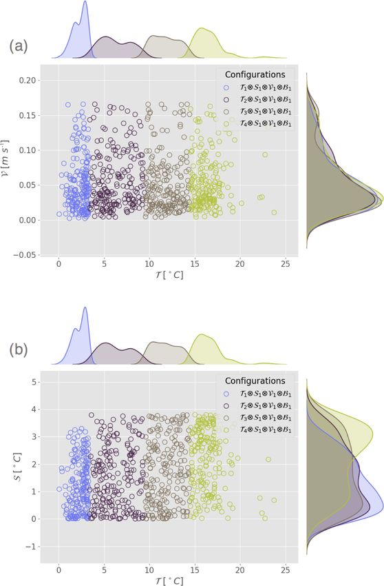
834                                  A. Delpech et al.: Influence of oceanic conditions in micronekton biomass estimation

priority is to collect observations and develop methods and       pilation of data found in the scientific literature (Lehodey
models needed to simulate and quantify the dynamics and           et al., 2010). Therefore, the largest uncertainty remains on
functional roles of these species’ communities.                   the energy transfer efficiency coefficients that control the to-
   Observations and biomass estimations of micronekton rely       tal abundance of each functional group.
traditionally on net sampling and active acoustic sampling           A method to estimate the model parameters has been de-
(e.g., Handegard et al., 2009; Davison, 2011). Each method        veloped using a maximum likelihood estimation (MLE) ap-
has limitations. Micronekton species can detect approaching       proach (Senina et al., 2008). A first study has shown that
fishing trawls, and part of them can move away to avoid           this method can be used to estimate the parameters Ei0 using
the net. This phenomenon leads to biomass underestima-            relative ratios of the observed acoustic signal and predicted
tion from net trawling (Kaartvedt et al., 2012). Conversely,      biomass in the three vertical layers during daytime and night-
acoustic signal intensity may overestimate biomass due to         time (Lehodey et al., 2015). However, this study was con-
presence of organisms with strong acoustic target strength,       ducted for a single transect in the very idealized framework
e.g., species that have gas inclusion inducing strong reso-       of twin experiments. While improved estimates of micronek-
nance (Davison, 2011; Proud et al., 2017). Improvements in        ton biomass are expected to become available in the coming
biomass estimation are expected in the coming years thanks        years, this will likely still require costly operations at sea.
to the combined use of different measurement techniques:          Therefore, it is important to assess realistically and more sys-
multiple acoustic frequencies, traditional net sampling and       tematically how well observations can estimate parameters
optical techniques (Kloser et al., 2016; Davison et al., 2015).   before deploying any observational system.
The accuracy of biomass estimates is predicted to benefit            For this purpose, we use Observing System Simulation
from this combination of techniques and from the develop-         Experiments (OSSEs, Arnold and Dey, 1986). This method
ments of algorithms that can attribute the acoustic signal to     allows for simulating synthetic observations in places where
biological groups.                                                real observations do not exist and allows us to examine how
   While these techniques for collecting observational esti-      useful the information they would provide is. The objective
mates of biomass are progressing, new developments are also       of the present study is to identify sampling regions, charac-
achieved in the modeling of the micronekton components            terized by different oceanic variables, at a global scale, in
of the ocean ecosystem. SEAPODYM (Spatial Ecosystem               which micronekton biomass observations provide the most
And Population Dynamics Model) is an Eulerian ecosys-             useful information for the model energy transfer coefficient
tem model that includes one lower- (zooplankton) and six          estimation. A set of synthetic observations is generated with
midtrophic (micronekton) functional groups and detailed fish      SEAPODYM using a reference parameterization. Then, the
populations (Lehodey et al., 1998, 2008, 2010). Given the         set of parameter values is changed, and an error is added to
structural importance of DVM, the micronekton functional          the forcing field in order to simulate more realistic condi-
groups are defined based on the daily migration behavior of       tions for parameter estimation. The MLE is used to estimate
organisms between three broad epi- and mesopelagic bioa-          the set of parameters from the set of synthetic observations.
coustic layers (Lehodey et al., 2010, 2015). In addition to       The difference between the reference and estimated parame-
DVM, the horizontal dynamics of biomass in each group is          ters provides a metric to select the best sampling zones. A
driven by ocean dynamics, while a diffusion coefficient ac-       method based on the clustering (Jain et al., 1999) of four
counts for local random movements. The source and sink for        oceanic variables of interest (temperature, current velocity,
the micronekton biomass are the recruitment from the poten-       stratification and productivity) is presented to investigate the
tial production of micronekton at a given age and the natural     sensitivity of the parameter estimation to the oceanographic
mortality, respectively. The recruitment time and the natu-       conditions of the observation regions. This method aims at
ral mortality of organisms are linked to the temperature in       determining which conditions are the most favorable for col-
the vertical layers inhabited by each functional group dur-       lecting observations in order to estimate the energy transfer
ing day or night. These mechanisms are simulated with a           efficiency coefficients.
system of advection–diffusion–reaction equations (Lehodey            The paper is organized as follows: Sect. 2 describes the
et al., 2008). The equations governing the model are de-          model setup and forcings as well as the method developed
tailed in Appendix A. Primary production is the source of         to characterize regions of observations and the metrics used
energy distributed to each group according to a coefficient       to evaluate the parameter estimation. Section 3 describes the
of energy transfer efficiency. Eleven parameters control the      outcome of the clustering method to define oceanographic
biological processes: a diffusion coefficient, six coefficients   regimes and synthesizes the main results of our estimation
(Ei0 )i∈{1...6} of energy transfer from primary production to-    experiments. The results are then discussed in Sect. 4 in the
ward each midtrophic functional group, and four parame-           light of biological and dynamical processes. Some applica-
ters for the relationship between water temperature and times     tions and limitations of our study are also identified along
of development (two parameters for the life expectancy and        with suggestions for possible future research.
two parameters for the recruitment time) (Lehodey et al.,
2010). The latter four parameters were estimated from a com-

Biogeosciences, 17, 833–850, 2020                                                       www.biogeosciences.net/17/833/2020/
A. Delpech et al.: Influence of oceanic conditions in micronekton biomass estimation 835
2 Method ity and primary production fields are depth-averaged over the
water column of each of the three layers defined by z1 , z2 and
2.1 The SEAPODYM-MTL model z3 , ending with a set of three-layered forcings fields. Initial
conditions of SEAPODYM-MTL come from a 2-year spinup
SEAPODYM-MTL (midtrophic levels) simulates six func- based on a monthly climatology simulation. Reference val-
tional groups of micronekton in the epipelagic and upper and ues of SEAPODYM-MTL parameters are those published in
lower mesopelagic layers at a global scale. These layers en- Lehodey et al. (2010). Overall the simulation reproduces the
compass the upper 1000 m of the ocean. The euphotic depth dynamics of the ocean well, but due to the low 1◦ horizon-
(zeu ) is used to define the depth boundaries of the vertical tal resolution, mesoscale features like eddies are not repre-
layers. These boundaries are defined as follows (an approxi- sented. The simulation captures the main temporal variability
mate average depth is given in brackets): z1 (x, y, t) = 1.5 × with a seasonal cycle in primary production and DVM cycle
zeu (x, y, t) (∼ 50–100 m), z2 (x, y, t) = 4.5 × zeu (x, y, t) (∼ for micronekton.
150–300 m), and z3 (x, y, t) = min(10.5 × zeu (x, y, t), 1000)
(∼ 350–700m), where zeu is given in meters. The six func- 2.2 Clustering approach to characterize potential
tional groups are called (1) epi (for organisms perma- sampling regions
nently inhabiting the epipelagic layer), (2) umeso (for organ-
isms permanently inhabiting the upper mesopelagic layer), We define the spatiotemporal discrete observable space as
(3) ummeso (for migrant umeso, organisms inhabiting the the set of the 1◦ × 1◦ grid points belonging to SEAPODYM-
upper mesopelagic layer during the day and the epipelagic MTL discrete domain. Each observation point is character-
layer at night), (4) lmeso (for organisms permanently in- ized by four indicators which are based on the following
habiting the lower mesopelagic layer), (5) lmmeso (for mi- environmental variables: the depth-averaged temperature T ,
grant lmeso, organisms inhabiting the lower mesopelagic a stratification index S, the surface velocity norm V and a
layer during the day and the upper mesopelagic layer at bloom index B, for which different regimes of intensity are
night) and (6) lhmmeso (for highly migrant lmeso, organ- defined. The averaged temperature T over the water column
isms inhabiting the lower mesopelagic layer during the day is defined as
and the epipelagic layer at night). The model is forced by cur- 1
T (x, y, t) = (T1 (x, y, t) + T2 (x, y, t) + T3 (x, y, t)) , (1)
rent velocities, temperature and net primary production (see 3
Appendix A for detailed equations).
where Tk is the depth-averaged temperature over the kth
This work is based on a 10-year (2006–2015) simula-
trophic layer of the model. The stratification index S is de-
tion of SEAPODYM-MTL, hereafter called the nature run
fined as the absolute difference of temperature between the
(NR). Euphotic depth, horizontal velocity and temperature
surface and subsurface layers:
fields come from the ocean dynamical simulation FREE-
GLORYS2V4 produced by Mercator Ocean. FREEGLO- S(x, y, t) = |T1 (x, y, t) − T2 (x, y, t)|. (2)
RYS2V4 is the global, nonassimilated version of the GLO-
RYS2V4 (http://resources.marine.copernicus.eu/documents/ The surface velocity norm V is defined as
QUID/CMEMS-GLO-QUID-001-025.pdf, last access: 7 q
January 2020) simulation that aims at generating a syn- V(x, y, t) = u21 (x, y, t) + v12 (x, y, t), (3)
thetic mean state of the ocean and its variability for oceanic
variables (temperature, salinity, sea surface height, currents where u1 and v1 are the zonal and meridional components of
speed, sea-ice coverage). It is produced using the numer- the depth-averaged velocity, respectively, in the first layer of
ical model NEMO (https://www.nemo-ocean.eu/, last ac- the model. The phytoplankton bloom index B is defined fol-
cess: 7 January 2020) with the ORCA025 configuration lowing Siegel et al. (2002) and Henson and Thomas (2007)
(eddy-permitting grid with 0.25◦ horizontal resolution and as a Boolean: 1 for bloom regions and 0 for no-bloom regions
75 vertical levels; see Barnier et al., 2006) and forced with based on temporal variations of primary production exceed-
the ERA-Interim atmospheric reanalysis from the ECMWF ing a threshold based on its annual median. More precisely,
(https://www.ecmwf.int/, last access: 7 January 2020). The we define
net primary production is estimated using the Vertically
1 if there exists t such that
Generalized Production Model (VGPM) of Behrenfeld and
|PP(x, y, t) − PP(x,
f y)|
Falkowski (1997) with satellite-derived chlorophyll-a con- B(x, y) = (4)
> 0.05 × PP(x, y),
f
centration. This product is available at the Ocean Produc-
0 elsewhere,
tivity home page of the Oregon State University (http:
//www.science.oregonstate.edu/ocean.productivity/, last ac- where PP(x,
f y) is the temporal median of the primary pro-
cess: 7 January 2020). Due to high computational demand, duction PP(x, y, t) at point (x, y). Note that, contrary to the
the original resolution of the simulation of 0.25◦ × week has previous indicator variables, the bloom index does not de-
been degraded to 1◦ × month. Temperature, horizontal veloc- pend on time. For each indicator variable G ∈ {T , S, V, B}
www.biogeosciences.net/17/833/2020/ Biogeosciences, 17, 833–850, 2020
836 A. Delpech et al.: Influence of oceanic conditions in micronekton biomass estimation
we define several ordered value-based regimes. The number
of regimes and regime boundary values are obtained by par-
titioning the set GN of the values of the indicator variable G
at N observable locations constituting an ensemble SN ⊂ .
GN = {gi = G(Xi ) Xi ∈ SN }1≤i≤N (5)
The partition of GN is computed using k-means clustering
(Kanungo et al., 2002). The k-means clustering method sep-
arates N points in a given number of cluster by minimizing
the distance of each point to the mean (called the center) of
each cluster. The number n of clusters is chosen according
to the elbow score (Kodinariya and Makwana, 2013; Tibshi-
rani et al., 2001). The k-means method produces n clusters Figure 1. A schematic view of the OSSE system. The synthetic
(0k )k∈{1...n} (called indicator variable regimes) that satisfy observations are generated using the simulation with the reference
the following properties: configuration (nature run). The control run is used to perform the es-
timation experiments. The evaluation of the OSSE is done by com-
Sn paring the estimated parameters with the reference parameters.
k=1
T 0k = GN and ∀i, j ∈ {1. . .n}, i 6 = j,
0i 0j = ∅ (6)
∀i ∈ {1. . .N }, gi ∈ 0k if k = argminkgi − µl k,
2.3.1 Nature and control runs and assimilation module
l∈{1...n}
where µl is the mean of values in 0l . Note that 0k depends The nature run (NR) used to perform the OSSE is generated
on the variable G. In the following, we make this dependence using the reference configuration of SEAPODYM-MTL de-
explicit by denoting 0k (G). The k-means clustering method scribed in Sect. 2.1. The NR is used to compute synthetic ob-
allows for size-varying clusters compared to more classical servations. The goal is then to retrieve the reference energy
statistical analyses that would consist, for example, of defin- transfer coefficients of the six micronekton functional groups
ing the regimes as the quantile of the variable distributions. Ei0 by assimilating the synthetic observations into a different
The latter could lead to underestimating (or overestimating) simulation of SEAPODYM-MTL, called the control run.
some identified regimes. The same kind of problem would The control run (CR) used to perform the parameter esti-
arise from a classification defined by traditional ecoregions mate is generated using perturbed forcing fields (Fig. 1). A
(Longhurst, 1995; Sutton et al., 2017), which would not ac- perturbation is added to the reference forcing fields in order
count for the specificity of our forcing fields. This is why to consider more realistically the discrepancy between the
performing a clustering to determine the different regimes real state of the ocean (represented here by the NR) and the
associated with the forcing fields seems a more rigorous ap- simplified representation of this state by numerical models.
proach here. The reference forcing fields are perturbed with a white noise
We define a configuration as the intersection of a selection whose maximal amplitude is a fraction of the averaged fields.
of regimes of given indicator variables. For i ∈ {1. . .nT }, j ∈ Let F be the considered forcing field and let F be its global
{1. . .nS }, k ∈ {1. . .nV } and l ∈ {1. . .nB }, the configuration C average (in space and time); we define the perturbed field as
is defined as
F
e(x, y, t) = F (x, y, t) + γ (αF ), (8)
C = Ti ⊗Sj ⊗Vk ⊗Bl = 0i (T )∩0j (S)∩0k (V)∩0l (B), (7)
where α ∈ [0, 1] is the amplitude of the perturbation and γ ∈
where nG is the number of clusters for the indicator variable [−1, 1] is a uniformly distributed random number. The am-
G. For the sake of simplicity we may also say that an obser- plitude α is set to 0.1 for all experiments except in Sect. 3.4,
vation point belongs to a configuration when the values of the where α varies. For small values of F , this perturbation can
indicator variables at this point belong to the corresponding induce a sign reversal of the forcing. This does not matter for
regimes of the configuration. Each configuration corresponds the temperature (degree Celsius; see also Eqs. A5 and A6)
to a subset SM ⊂ SN of observable points. or the current velocities (meter per second); primary produc-
tion (millimoles of carbon per squared meter per day) has
2.3 OSSE system configuration however been constrained to positive values. White noise has
been preferred to more realistic perturbation to avoid any ge-
To perform realistic OSSEs, a rigorous protocol needs to be ographical bias pattern. The implications of this choice are
followed (Hoffman and Atlas, 2016). Here, we describe the further discussed in Sect. 4.3. Its amplitude, fixed to 10 % of
different steps. A scheme summarizing the OSSE methodol- error, is however representative of the mean error estimated
ogy is given in Fig. 1. for ocean circulation models (Lellouche et al., 2013; Gar-
Biogeosciences, 17, 833–850, 2020 www.biogeosciences.net/17/833/2020/
A. Delpech et al.: Influence of oceanic conditions in micronekton biomass estimation                                                     837

Table 1. SEAPODYM-MTL parameters used for the two different simulations: the nature run (NR) and the control run (CR). E is the energy
transferred by net primary production to intermediate trophic levels, λ is the mortality coefficient, τr is the minimum age to be recruited in
the midtrophic functional population, and D is the diffusion rate that models the random dispersal movement of organisms. Ei0 , i ∈ {1, 6} are
the redistribution energy transfer coefficients to the six components of the micronekton population. The parametrization of the NR is called
the reference parametrization and is taken from Lehodey et al. (2010).

           Simulation     1/λ (d)   τr (d)   D (NM2 d−1 )           E        E10     E20       E30    E40      E50    E60    Forcing
           NR               2109      527                15    0.0042    0.17       0.10     0.22 0.18        0.13   0.20          F
           CR               2109      527                15    0.0042                         first guess                   e (Eq. 8)
                                                                                                                            F

ric and Parent, 2017). The parameters Ei0 are randomly sam-              2.4       OSSE system evaluation metrics
pled between 0 and 1. This first guess is used as initialization
of the optimization scheme. We run each experiment several               The estimation experiments are evaluated using three met-
times with a different randomly sampled first guess in order             rics: (i) the performance of the estimation, (ii) its accuracy
to ensure that the inverse model is not sensitive to the ini-            and (iii) its convergence speed.
tial parameters. The setup of the NR and CR simulations is
                                                                             (i) The performance is measured with the mean relative er-
summarized in Table 1.
                                                                                 ror between the estimated coefficients and the reference
   A MLE is used as an assimilation module, used here to
                                                                                 coefficients as defined in Lehodey et al. (2015) (Eq. 9).
estimate model parameters from observations. Its implemen-
tation is based on an adjoint technique (Errico, 1997) to it-                                 6  b0 − E 0
                                                                                           1X    Ei     i
eratively optimize a cost function that represents the discrep-                    Er =                   .                               (9)
ancy between model outputs and observations. This approach                                 6 i=1    Ei0
conforms to current practices. More details about the imple-
mentation of this approach in SEAPODYM can be found in                    (ii) The accuracy is measured by the residual value of
Senina et al. (2008) and Lehodey et al. (2015).                                the likelihood which provides a good estimate of the
                                                                               discrepancy between the estimated and the observed
2.3.2   Synthetic observations                                                 biomass.

In the framework of OSSE, we perform estimation experi-                  (iii) The convergence speed is measured by the iteration
ments with different sets of synthetic observation points of                   number of the optimization scheme.
size Ne = 400. The synthetic observations are sampled from
the different configurations introduced in the previous sec-                The residual likelihood and iteration number metrics are
tion. Let M be the number of points in a given configuration.            provided by the Automatic Differentiation Model Builder
If M < Ne , we consider that the configuration is too singu-             (ADMB) algorithm (Fournier et al., 2012) that is used to
lar to be relevant for our study and it is ignored. If M > Ne ,          implement the MLE. Each metric provides different and in-
we randomly extract a subsample SNe ⊂ SM of observation                  dependent information. For example, it is possible to obtain
points. In order to study the influence of one indicator at a            good performance and bad accuracy with an experiment that
time, we compare experiments for which the regime of the                 estimates correctly the energy transfer parameters for the dif-
studied indicator varies and the regime of the other indica-             ferent functional groups but over- or underestimates the total
tor variables remains fixed. In the following we call primary            amount of biomass. The performance is generally used to dis-
variable the studied indicator variable and secondary vari-              criminate between the different experiments since the aim of
ables the ones whose regimes are fixed. For a given group of             the study is to find the networks that better estimate energy
experiments, we check that the configurations are compara-               transfer coefficients and thus directly minimize the error Er
ble to each other by ensuring that the distribution of all sec-          (Eq. 9). However, the accuracy and precision of the experi-
ondary variables is similar (see marginal distribution plots in          ment are also discussed below. The convergence is necessary
Sect. 3.2.1). If this not the case, they are not reported. A ran-        to ensure that the optimization problem is well defined.
dom sampling of observations within each configuration is
preferred to a more realistic observation network to avoid any           3     Results
geographical bias. But this choice is discussed in Sect. 3.4,
where realistic networks are tested. The coverage in terms               3.1       Environmental regimes clustering
of observation numbers is however quite realistic. We use
400 observations in our experiments, which at the resolution             The number of points per regime, obtained from the cluster-
of the model (1◦ × 1 month) correspond, for example, to the              ing (Sect. 2.2) and defined for each environmental variable
deployment of six moorings during 5 years.                               (Table 2), shows a large variability. Some regimes represent a

www.biogeosciences.net/17/833/2020/                                                                         Biogeosciences, 17, 833–850, 2020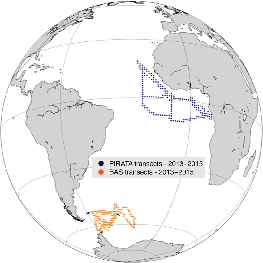
838                                      A. Delpech et al.: Influence of oceanic conditions in micronekton biomass estimation

Figure 2. Spatial division of the different regimes as defined in Table 2. (a) Temperature: polar (pale blue), subpolar (yellow), temperate
(gray) and tropical (red). (b) Stratification: weak (dark blue), intermediate (purple) and strong (magenta). (c) Current velocities: low (blue)
and high (orange). (d) Bloom index: bloom (green) and no bloom (beige). Each point of the subset SN has been plotted at its spatial location
with a color corresponding to the regime it belongs to.

larger amount of observable points. For instance, the tropical-           highlight the main energetic structures of the oceanic circula-
temperature regime covers 31 % of the observable points. Al-              tion. The high-surface-current regime thus covers the intense
most 50 % of the observable points show a weak stratifica-                jet-structured equatorial currents, the western boundary cur-
tion and only 10 % of them have a positive bloom index or                 rents (the Gulf Stream in the Atlantic and the Kuroshio in
high velocities. When they are shown on a map (Fig. 2) these              the Pacific), the Agulhas Current along the South African
regimes reproduce classical spatial patterns described in the             coast and the Antarctic Circumpolar Current in the Southern
scientific literature (Fieux and Webster, 2017). The regimes              Ocean. The regimes of the bloom index (B) separate mostly
of the temperature variable (T ) show a latitudinal distribu-             the productive regions (North Atlantic and North Pacific,
tion. The polar regime (T1 ) is located south of the polar front          Southern Ocean, eastern side of the tropical Atlantic, along
(Southern Hemisphere) and in the Arctic Ocean. The subpo-                 the African coast) from the nonproductive regions (center of
lar regime is located between the polar front and the south               subtropical gyres mostly, as well as coastal regions of the
tropical front (Southern Ocean), in the subpolar gyre region              Arctic and Antarctic).
(North Atlantic), and in the Bering Sea (North Pacific). The                 Based on these results, we construct all possible configu-
temperate regime covers the subtropical zones of the South-               rations, using the methodology described in Sect. 2.2. Then
ern Atlantic, Indian and Pacific oceans, located north of the             the configurations are selected to perform the OSSEs pre-
south tropical front, and extends as well in the eastern part             sented in Sect. 2.3. The choice of the configuration is lim-
of the Atlantic and Pacific Ocean. The tropical regime covers             ited by the number of observation points available in each of
most of the tropical ocean and the Indian Ocean. The regimes              them. Among the 48 possible configurations, 21 of them are
of the stratification variable (S) are also structured according          nearly empty as they contain less than 0.5 % of all observ-
to the latitude, as stratification depends on the temperature.            able points. They are thus considered nonexistent. In addi-
The stratification decreases from the tropical oceans (where              tion, we study the influence of the primary variable by select-
the surface waters are warm compared to the deep waters) to               ing only groups of configurations whose distributions along
the pole (where the surface waters are almost as cold as the              secondary variables are similar. This leads to a selection of
deep waters). The regimes of the surface velocity norm (V)                seven groups of experiments (Table 3). The purpose of the

Biogeosciences, 17, 833–850, 2020                                                                 www.biogeosciences.net/17/833/2020/
A. Delpech et al.: Influence of oceanic conditions in micronekton biomass estimation 839
first three groups of Experiment 1a–b, c–d and e–f is to study
Table 2. Outcome of the clustering method (Sect. 2.2). For each indicator variable (temperature T , stratification S, velocity V and bloom index B), the number n of clusters, and the
the influence of the velocity regimes V1 and V2 . The group of
no bloom
3 730 655
89.2 %
B2
18.4 mmol C m−2 d−1
Experiment 2a–d is used to study the influence of the temper-
ature regimes T1 , T2 , T3 and T4 . The group Experiment 3a–c
is used to investigate the influence of the stratification index
Bloom index (B; n = 2) regimes S1 , S2 and S3 . Finally, Experiment 4a–b and c–d
evaluate the impact of the bloom index regimes B1 and B2 .
3.2 Estimation performance with respect to
bloom
449 545
10.8 %
B1
74.6 mmol C m−2 d−1
environmental conditions
Table 3 shows the selected configurations for each experi-
ment (usually abbreviated as Exp. in the following) as well
as their evaluation metrics. All experiments converged after
16 to 28 iterations. This confirms that the optimization prob-
lem is well defined. Since the number of iterations is partially
dependent on the random initial first guess, it is not used as a
center and size (no. observable) of each cluster (regimes) are given, as well as the proportion of all observable points it represents.
high
481 367
11.5 %
V2
0.3 m s−1
Velocity (V; n = 2)
criterion of discrimination between experiments.
3.2.1 Influence of the horizontal current velocity
low
3 698 826
88.5 %
V1
0.05 m s−1
The influence of the current velocity regimes (high-current-
velocity system or low-current-velocity system) on the per-
formance of the parameter estimation is studied considering
strong
11.7 ◦ C
882 949
21.1 %
S3
three groups of experiments (Table 3, Exp. 1a to f). The ob-
servation points are randomly sampled in a subset of the con-
Stratification (S; n = 3)
sidered configuration for which the primary variable is the
current velocity norm V.
inter.
5.9 ◦ C
1 212 945
29.0 %
S2
From these sets of experiments, it appears that the per-
formance of the parameter estimation decreases with higher
current velocity at the observation points. This conclusion
weak
0.4 ◦ C
2 084 302
49.8 %
S1
is valid regardless of the regime of the secondary variables:
either low or high temperatures, positive or null bloom in-
dex, and weak or strong stratification (Table 3). Lower ve-
locity reduces the error on the estimated energy transfer co-
tropical
16.3 ◦ C
1 300 298
31.1 %
T4
efficients for functional groups that are impacted by currents
in the epipelagic and upper mesopelagic layers. The currents
decrease with depth and are almost uniform over the dif-
Temperature (T ; n = 4)
ferent regions in the lower mesopelagic layer (not shown).
temperate
12.6 ◦ C
1 115 102
26.7 %
T3
Consequently, the estimate of the parameters for the nonmi-
grant lower mesopelagic (lmeso) group is not sensitive to the
regime of currents (Fig. 3a). Conversely, the estimation is the
subpolar
6.4 ◦ C
658 105
15.7 %
T2
most sensitive for the epipelagic group, whose dynamics are
entirely driven by the surface currents.
Note that the influence of low and high velocities is not
explored for all secondary-variable fixed regimes. Indeed,
polar
0.4 ◦ C
1 106 695
26.5 %
T1
even within fixed regimes, the secondary-variable distribu-
tion along observation points might not be statistically com-
parable between two experiments. This could lead to a po-
Number observable
tential bias introduced by a secondary variable, which is not
Regime names of
0k (G), k ∈ {1, n}
the target of the study. For instance, the influence of velocity
Cluster center
in a polar temperature regime can be investigated by compar-
Proportion
ing the configurations C 0 = T1 ⊗ S1 ⊗ V1 ⊗ B2 (low velocity)
in cluster
Regimes
and C 00 = T1 ⊗S1 ⊗V2 ⊗B2 (high velocity). The correspond-
ing estimation experiments (Exp. 10 and Exp. 100 ) give rela-
www.biogeosciences.net/17/833/2020/ Biogeosciences, 17, 833–850, 2020840 A. Delpech et al.: Influence of oceanic conditions in micronekton biomass estimation Figure 3. Mean relative error (Er in %, Eq. 9) on each Ei0 coefficients for (a) Exp. 1c and d, which present the following tested regimes: high versus low velocities in temperate temperatures, weak-stratification regimes and bloom regimes; (b) Exp. 2a, 2b, 2c and 2d, which compares polar, subpolar, temperate and tropical temperatures in weak-stratification, low-velocity and bloom regimes; (c) Exp. 3a, b and c, which compares weak, intermediate and high stratification in tropical-temperature, low-velocity and no-bloom regimes; and (d) Exp. 4c and d: bloom versus no-bloom regimes in tropical temperatures, strong stratification and low velocities. tive errors of 48 % and 10 % respectively. This result seems iments with significant cross-correlation between indicator contradictory to the conclusions drawn from Exp. 1a–f. But variables are not presented; this concerns 9 out of the 26 pos- looking at the distributions of the observations along the sec- sible experiments. ondary variables, we can notice that the temperatures are dif- ferent between the two configurations. While both configu- rations are considered to be in the polar regime, the temper- 3.2.2 Influence of temperature ature in configuration C 0 (−0.7 ◦ C) is on average lower than the temperature of configuration C 00 (2.1 ◦ C) (Fig. 4). Thus In Exp. 2a to d (Table 3), temperature is the primary variable, Exp. 10 and Exp. 100 measure the combined effect of both ve- ranging from polar regime (Exp. 2a) to subpolar (Exp. 2b), locity and temperature. The lower velocities are coupled with temperate (Exp. 2c) and tropical (Exp. 2d) regimes. All lower temperatures and the higher velocities with higher tem- other indicator variables (stratification, velocity and bloom peratures. There is a cross-correlation between the velocity index) are secondary variables that are set to weak, low (primary variable) and the temperature (secondary variable). and 1 respectively. Figure 5 shows that the distributions Therefore, it is not possible to assess the influence of the ve- along the secondary variables of each configuration are close locity on the parameter estimation from these experiments. enough for the experiments to be compared, avoiding any Although the distributions of the secondary variables are risk of cross-correlation. The performance of the estimation not always shown in the following experiments, they have increases with the temperature (Fig. 3b). The mean error been examined to ensure that the OSSE results are not biased on the parameter estimates decreases respectively from po- by systematic differences in the secondary variables. Exper- lar (Exp. 2a; 9.1 %) to subpolar (Exp. 2b; 7 %), temperate Biogeosciences, 17, 833–850, 2020 www.biogeosciences.net/17/833/2020/
A. Delpech et al.: Influence of oceanic conditions in micronekton biomass estimation 841
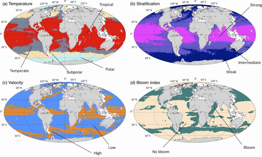
Figure 4. Scatter plot and marginal distribution from kernel den-
sity estimation (Silverman, 2018) in the plane (V,T ) of observation
points used in Exp. 10 and Exp. 100 generated by random sampling in
configurations C 0 = T1 ⊗S1 ⊗V1 ⊗B2 and C 00 = T1 ⊗S1 ⊗V2 ⊗B2 .
(Exp. 2c; 3 %) and tropical (Exp. 2d; 1.4 %) configurations
(Table 3).
3.2.3 Influence of stratification
The influence of stratification is first investigated with a set
of three configurations combining the tropical-temperature
regime; low-velocity regime; null bloom index regime; and
three regimes of weak (Exp. 3a), intermediate (Exp. 3b) and
strong (Exp. 3c) stratification. A marginal distribution plot
of observation sets for all experiments (not shown) indi- Figure 5. Scatter plot and marginal distribution from kernel density
cates that the three datasets differ only along the stratifica- estimation in the plane (a) (T ,V) and (b) (T ,S) for the configura-
tion variable (primary variable). The observation points dis- tions corresponding to Exp. 3a, b, c and d from Table 3.
play a temperature between 14 and 17 ◦ C, a velocity between
0 and 0.07 m s−1 and a null bloom index for each experi-
ment. The performance decreases with the intensity of strat-
3.2.4 Influence of primary production
ification (Fig. 3c and Table 3). The mean error is 3.5 % for
a weak stratification and a vertical gradient of about 0.4 ◦ C
(Exp. 3a), 5.9 % for an intermediate stratification with a gra- In order to investigate the influence of primary production
dient of about 5.9 ◦ C (Exp. 3b) and 8 % for a strong stratifica- on the performance of the estimation, we compare the results
tion around 11.7 ◦ C (Exp. 3c). A strong stratification seems of estimation in configurations with different bloom index
to deteriorate the estimate for all migrant groups (Fig. 3c). regimes (primary variable). Temperature, stratification index
These results are not specific to the choice of regimes for the and velocity have been fixed (secondary variables) to sub-
secondary variables. Similar experiments were carried out in polar, weak, and low regimes respectively (Exp. 4a and b)
a temperate regime (not shown), and, even though the mean and to tropical, strong, and low regimes for Exp. 4c and d.
error on the estimated parameters is higher on average, the re- Distributions of the observation points along the secondary
sult does not change: weak stratification again leads to a bet- variables indicate that the experiments are not biased by sec-
ter estimation than strong stratification. The comparison was ondary variables, as the distributions present similar modes
not fully possible in other temperature or velocity regimes centered at 5 ◦ C for the temperature; at 0.5 ◦ C for the strati-
because these configurations are not sufficiently represented. fication index; at 0.04 m s−1 for the velocity (Exp. 4a and b);
and at 15.5, 11 ◦ C and 0.05 m s−1 respectively for Exp. 4c
and d (not shown).
Both Exp. 4a and b result in an averaged error of 7 %
on the estimated parameters (Table 3). Experiment 4d (av-
www.biogeosciences.net/17/833/2020/ Biogeosciences, 17, 833–850, 2020842 A. Delpech et al.: Influence of oceanic conditions in micronekton biomass estimation
Table 3. Experiment table. List of conducted experiments, their corresponding configurations and the evaluation diagnostics: mean relative
error on the coefficients, residual likelihood and number of iterations. The tested regime (primary variable) is specified in the first column,
the number of observable belonging to each configuration is indicated in the fourth column, with their relative proportion in brackets. Note
that, even if the number of observable points differs for each configuration, the experiments were conducted with 400 observations randomly
chosen among the ones belonging to the configuration. The section that describes each experiment is mentioned in the last column.
Experiment Configuration Number observable Er (Eq. 9) Residual Number of Section
likelihood iterations
Velocity (V) 1a T2 ⊗ S1 ⊗ V1 ⊗ B2 317 695 (7.6 %) 7.0 % 0.9 28 3.2.1
1b T2 ⊗ S1 ⊗ V2 ⊗ B2 54 343 (1.3 %) 9.7 % 0.5 21
1c T3 ⊗ S1 ⊗ V1 ⊗ B1 112 865 (2.7 %) 3.1 % 0.5 24
1d T3 ⊗ S1 ⊗ V2 ⊗ B1 397 119 (9.5 %) 8.3 % 1.5 23
1e T4 ⊗ S3 ⊗ V1 ⊗ B1 401 299 (9.6 %) 1.5 % 1.1 16
1f T4 ⊗ S3 ⊗ V2 ⊗ B1 146 307 (3.5 %) 8.5 % 1.2 18
Temperature (T ) 2a T1 ⊗ S1 ⊗ V1 ⊗ B1 982 347 (23.5 %) 9.1 % 1.7 19 3.2.2
2b T2 ⊗ S1 ⊗ V1 ⊗ B1 175 568 (4.2 %) 7.0 % 0.6 26
2c T3 ⊗ S1 ⊗ V1 ⊗ B1 112 865 (2.7 %) 3.1 % 1.3 20
2d T4 ⊗ S1 ⊗ V1 ⊗ B1 58 522 (1.4 %) 1.4 % 0.6 22
Stratification (S) 3a T4 ⊗ S1 ⊗ V1 ⊗ B2 75 244 (1.8 %) 3.5 % 0.7 21 3.2.3
3b T4 ⊗ S2 ⊗ V1 ⊗ B2 91 964 (2.2 %) 5.9 % 0.8 25
3c T4 ⊗ S3 ⊗ V1 ⊗ B2 40 130 (0.9 %) 8.0 % 1.1 21
Bloom index (B) 4a T2 ⊗ S1 ⊗ V1 ⊗ B1 175 568 (4.2 %) 7.0 % 0.6 26 3.2.4
4b T2 ⊗ S1 ⊗ V1 ⊗ B2 317 695 (7.6 %) 7.0 % 0.9 28
4c T4 ⊗ S3 ⊗ V1 ⊗ B1 401 299 (9.6 %) 1.5 % 0.6 22
4d T4 ⊗ S3 ⊗ V1 ⊗ B2 40 130 (0.9 %) 8.0 % 0.8 21
eraged error of 8 %) gives a similar value to Exp. 4b. Indeed, along the main currents). The signature of the Antarctic Cir-
Exp. 4d (T4 regime) has a higher temperature than Exp. 4b cumpolar Current is found in the Southern Ocean with an er-
(T2 regime), but it also has a higher stratification index (the ror over 10 %. Similarly, the signature of the North Atlantic
S3 regime for Exp. 4d and the S1 regime for Exp. 4b). Fol- Drift can be seen with a patch of high errors between Canada
lowing the conclusions from the two previous sections, better and Ireland (Figs. 2c and 6). The patch of high errors in the
performance is achieved when temperature increases, though North Pacific Ocean, however, is difficult to interpret. The
increasing stratification has the opposite effect. So, the two equatorial regions show interesting patterns that are similar
effects might compensate in this case and result in a sim- across the three oceans. In the vicinity of the Equator, good
ilar estimation. However, when considering bloom regions performances are observed (mean error ∼ 2 %). On both the
(Exp. 4c), the estimation error falls to 1.5 % on average. In northern and southern sides of this low error band, the per-
addition, this experiment estimates the energy transfer coef- formance is decreased, with errors reaching about 8 %. The
ficients for migrant micronekton groups with less than 1 % equatorial regions are characterized by strong currents and
error (Fig. 3d). According to our results, the primary produc- warm surface waters. As described above, these environmen-
tion and the regimes of the bloom index do not always play a tal features have opposite effects on the performance of the
role in the performance of the parameter estimation. A posi- estimation. Therefore, a possible explanation of this distri-
tive bloom index appears to improve the performance of the bution of errors is that water temperature is high enough
estimation at high temperatures only. to overcome the effect of currents in the equatorial band,
but when moving poleward the temperature decreases can-
3.3 Global map of parameter estimation errors not compensate anymore for the negative effect of currents,
which is still quite strong. It should be noted that the map
When considering all possible experiments, and given the presented in Fig. 6 was obtained for a given set of forcing
fact that all these configurations are associated with specific fields (temperature, velocity, primary production). It is thus
locations and times, it is possible to represent a global map of dependent on the simulation that is used. The regime depen-
averaged estimation errors (Eq. 9). This map (Fig. 6) shows dence of the estimation performance is however independent
that, on average, the error increases from the Equator to- of the simulation.
wards the poles. The lowest performances (errors > 40 %)
are mostly found in the Arctic and Southern Ocean. Low
performances are also found at some specific locations (e.g.,
Biogeosciences, 17, 833–850, 2020 www.biogeosciences.net/17/833/2020/A. Delpech et al.: Influence of oceanic conditions in micronekton biomass estimation 843
is very strong since PIRATA and BAS are both underway
ship measurements taken from 2-month cruises, repeated an-
nually. The results seem much less dependent on the exact
design of the samplings and the seasonality of the measure-
ments than on their actual geographical location. Oceanic
conditions of the observations (correlated to their geographi-
cal location) are the first order of sensitivity. In this sense, the
PIRATA network is thus a very promising observatory for the
micronekton, especially since it already includes a complete
set of various physical and biogeochemical parameter mea-
surements (Foltz et al., 2019).
4 Discussion
In the following, we will discuss a possible theoretical
Figure 6. Averaged absolute value of relative error (Er in %, Eq. 9)
between the estimated and the target energy transfer parameters
interpretation of the outcome of the estimation experi-
(Ei0 ) according to the location of the chosen observation points, as- ments (Sect. 4.1) and a potential application of our results
sociated with the forcing fields described in Sect. 2.1. Cells with no (Sect. 4.2). Section 4.3 closes this discussion examining the
data have been shaded in gray. particular framework used to conduct this study and opening
some perspectives for future work.
4.1 An interpretation of the performance in terms of
3.4 Testing realistic networks observability
The above experiments are based on random selection of ob- The differences in the performance of parameter estimation
servation points within a large subset. This technique was can be interpreted in the light of the characteristic timescales
chosen to avoid any bias related to the temporal or spatial of physical and biological processes. The parameters we
potential autocorrelation of observation networks. However, want to estimate (Ei0 ) control the energy transfer efficiency
sampling at sea is rarely randomly distributed and can gen- between the primary production (PP) and micronekton pro-
erate correlations. To relax this strong assumption, we per- duction (P ) (Eq. A3; Appendix A). These parameters are
form experiments based on positions from real acoustic tran- thus directly related to the relative amount (Pi ) of P in each
sects (underway ship measurements). Two regions are com- functional group i at age τ = 0, and we have
pared using the transects from the PIRATA cruises in the
equatorial Atlantic (Bourlès et al., 2019) and those from the Pi (τ = 0)
Ei0 = R , (10)
British Antarctic Survey (BAS) close to the Antarctic Penin- cEPP PPdz
sula (Fig. 7).
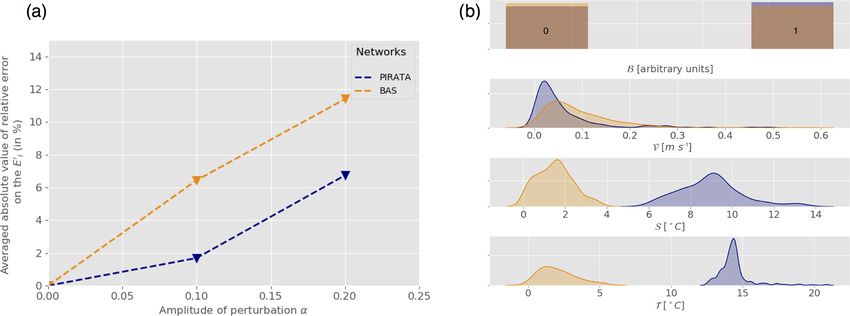
The same forcing, method and initial parameterization where EPP is the total energy transfer from the primary pro-
were used with a random noise amplitude (α) increasing duction to the midtrophic level (all functional groups to-
from 0 to 0.2. Subsets of Ne = 400 observations were se- gether) and c a conversion coefficient (see Appendix A). It is
lected along the transects to run the experiments. The result- possible to rewrite the initial condition (Eq. A3) as a system
ing averaged relative error on the coefficients is shown as a of six equations involving the energy transfer coefficients.
function of the amplitude of perturbation (Fig. 8a) for both
ρ1,d (P|τ =0 ) = E10 ,
networks. It appears that the estimation error increases with
ρ1,n (P|τ =0 ) = E10 + E30 + E60 ,
the amplitude of the error introduced on the forcing field.
ρ2,d (P|τ =0 ) = E20 + E30 ,
Also, regardless of the intensity of the perturbation, the es- (11)
ρ2,n (P|τ =0 ) = E20 + E40 ,
timation error is always lower when using PIRATA observa-
ρ3,d (P|τ =0 ) = E40 + E50 + E60 ,
tion networks than BAS observation networks. These results
ρ3,n (P|τ =0 ) = E40 ,
are fully consistent with the previous results indicating that
networks located in tropical warm waters, as for PIRATA, where ρK,ω (P|τ =0 ), with ρ defined as ρK,ω (P ) =
give better estimates than the ones located in cold waters, P
i|K(i,ω)=K Pi
as for the BAS (Fig. 8b). This should give confidence in the P6 , is the ratio of age 0 potential micronek-
i=1 Pi
fact that our results are robust when the random sampling hy- ton production in the layer K ∈ {1, 2, 3}, at the time of the
pothesis used in the previous section is relaxed and that more day ω ∈ {d, n} (for day and night).
realistic sampling designs are considered. Here in particu- The predicted micronekton biomass at a given time and
lar, the temporal autocorrelation of the different samplings location (grid cell) results from two main mechanisms. First,
www.biogeosciences.net/17/833/2020/ Biogeosciences, 17, 833–850, 2020844 A. Delpech et al.: Influence of oceanic conditions in micronekton biomass estimation
the potential production (P ) evolves in time from age τ = 0
and is redistributed by advection and diffusion until the re-
cruitment time τr when it is transferred into biomass (B).
Second, the biomass is built by the accumulation of re-
cruitment over time in each grid cell and is lost due to a
temperature-dependent mortality rate, while the currents re-
distribute the biomass spatially. The observations correspond
to the relative amount of biomass in each layer, i.e., the ra-
tios of biomass ρK,ω (B|t=t o ) (Eq. A7), where t o is the time
at which the observation is collected. Therefore, the observa-
tion will contain more information about the energy transfer
parameters we want to estimate if ρK,ω (B|t=t o ) is close to
ρK,ω (P|τ =0 ) (Eq. 11). This requires that the integrated mix-
ing and redistribution of biomass during the elapsed time
between age 0 of potential production and the time of ob-
servation (i.e., at least the recruitment time) are as weak as
possible. This can be achieved in two ways: either (i) the
currents are weak so that the advection of biomass is also
weak (but the diffusion will still remain) or (ii) the tem-
perature is high, leading to a short recruitment time with Figure 7. Map of PIRATA and BAS ship transects for the years
a reduced period of transport, mixing and redistribution of 2013–2015.
biomass (Eq. A5). These two mechanisms can explain why
warm temperatures and weak currents were found to improve is shorter than the one governing physical processes (τφ ) at
the estimations compared to cold temperatures and high ve- the location of the observation: τβ
τφ .
locities (Sect. 3.2.1 and 3.2.2). An additional effect of warm This interpretation highlights the problem of observabil-
temperature is that it induces a higher mortality rate (Eq. A6). ity of the parameters Ei0 from the measurements ρK, (B).
When warm waters are combined with high primary produc- The parameters are directly observable at the age τ = 0 of
tion (e.g., the equatorial upwelling region), there is a rapid the production, but the measurements and the information we
turnover of biomass, and the relative ratios of biomass by can get on the system are available only after a time τr . The
layer are closer to the initial ratio of production and thus observability will then be the better if the observable vari-
to the energy transfer efficiency coefficients. Conversely, at ables have not changed too much during the time τr (short
cold temperature, the mortality rate is lower; biomass is accu- τr , slow ocean dynamics). This is intrinsically linked to gov-
mulated from recruitment events and carries with it the inte- erning equations of the system (Eqs. A1–A3) and therefore
grated mixing and the perturbed ratio structures. This can ex- should not be dependent on the framework of the study.
plain why, at warm temperature, high productivity is needed
for a better estimation (Sect. 3.2.4). A side effect is that if 4.2 Towards ecoregionalization?
temperature is not homogeneous across layers, then the mor-
tality rate λ will differ for each functional group, depending The clustering approach we propose allowed the identifica-
on the layers it inhabits. This will be an additional driver of tion of oceanic regions that provide optimal oceanic char-
perturbation on the observed ratios of biomass compared to acteristics for our parameter estimation. It separates regions
the initial ratios of potential production. This is consistent where the distribution of biomass is driven by physical pro-
with the result that a strong thermal stratification degrades cesses from regions where it is driven by biological pro-
the performance of estimation (Sect. 3.2.3). cesses. This could be seen as a new definition of ecoregions
An observation will thus be the most effective for the esti- based on similar ecosystem structuring dynamics. The defi-
mation of parameters if it carries the information of the ini- nition of ocean ecoregions has been proposed based on vari-
tial distribution of primary production into functional groups. ous criteria (Emery, 1986; Longhurst, 1995; Spalding et al.,
This is the case if the biomass is renewed quickly enough 2012; Fay and McKinley, 2014; Sutton et al., 2017; Proud
compared to the time it takes for the currents and diffusive et al., 2017). A convergence of these different approaches to
coefficient to mix it. This condition can be seen in terms identify regions characterized by homogeneous mesopelagic
of equilibrium between the biological processes (production, species communities would be of great interest to facilitate
recruitment and mortality) and the physical processes (ad- the modeling and biomass estimate of the mesopelagic com-
vection and diffusion). For an observation to be the most ponents. Acoustic observation models could be developed
useful to the parameter estimation, it is necessary that the and validated at the scale of these regions. Then, the observa-
characteristic timescale governing biological processes (τβ ) tion models integrated into ecosystem and micronekton mod-
els as the one used here would serve to convert their predicted
Biogeosciences, 17, 833–850, 2020 www.biogeosciences.net/17/833/2020/A. Delpech et al.: Influence of oceanic conditions in micronekton biomass estimation 845
Figure 8. (a) Mean relative error on the coefficients Er (in %, Eq. 9) as a function of the perturbation amplitude α (Eq. 8) for PIRATA
(blue) and BAS (orange) observation networks. (b) Statistical distribution of all PIRATA (blue) and BAS (orange) observation location indi-
cator variables: bloom index (B), velocity norm (V), stratification index (S) and temperature (T ) estimated using kernel density estimation
(Silverman, 2018).
biomass into an acoustic signal to be directly compared to all ered sources of potential error: the correction with depth,
acoustic observations collected in the selected region. This the target strength of species, and the intercalibration be-
approach would allow us to account for (and estimate) the tween instruments and the signal processing methods (Han-
sources of biases and errors linked to acoustic observations degard et al., 2009, 2012; Kaartvedt et al., 2012; Proud et al.,
directly in the data assimilation scheme. 2018). This is an important research domain that requires the
combination of multiple observation systems, including new
4.3 Limitations and perspectives emerging technologies such as broadband acoustics, optical
imagery and environmental DNA to reduce overall bias in
estimates of micronekton biomass (e.g., Kloser et al., 2016)
We have chosen to model the error between the true state of
and use those estimates to assess, initiate and assimilate into
the ocean and the modeled state by adding a white noise per-
ecosystem models. Finally, the results of the clustering ap-
turbation to the forcings of the NR as input of the CR. Our
proach need to be confirmed with other ocean circulation
idealized approach does not take into account the possible
model outputs, especially at higher resolution to check the
spatial distribution of uncertainty and errors of ocean mod-
impact of the mesoscale activity on the definition of optimal
els, and other approaches would be interesting to explore. For
regions for energy transfer efficiency estimation. In a future
instance, implementing an error proportional to the deviation
study, in addition to testing the impact of introducing noises
of the climatological field should be more realistic because it
in the observations, the same approach could be used to also
would be based on the natural and intrinsic variability of the
directly estimate the model parameters that control the re-
ocean. Indeed, we expect forcing fields to be less accurate
lationship between the water temperature and the time of
where the ocean has strong variability. However, for the pur-
development of micronekton organisms. Other perspectives
pose of our study, a spatial homogeneous error was prefer-
may include a study of the sensitivity to the design of the
able to avoid introducing any bias. Random noise ensures
samplings (the impact of moored instruments in comparison
that the results obtained in different locations are directly
with underway measurements), in the continuity of the work
comparable. Conducing a sensitivity analysis with respect to
of Lehodey et al. (2015).
the choice of forcing error modeling was beyond the scope
of this study. In addition to the uncertainty of ocean model
outputs, other sources of uncertainties remain to be explored 5 Conclusions
to progress toward more realistic estimation experiments.
For instance, we considered that the observation operator Understanding and modeling marine ecosystem dynamics
(Eq. A7) is perfect but field observations are always tainted is considerably challenging. It generally requires sophisti-
by errors. The micronekton biomass estimates at sea require cated models relying on a certain number of parameterized
a chain of extrapolation and corrections to account for the physical and biological processes. SEAPODYM-MTL pro-
sampling gear selectivity and the portion of water layer sam- vides a parsimonious approach with only a few parameters
pled. For acoustic data, many factors need to be consid- and a MLE to estimates these parameters from observations.
www.biogeosciences.net/17/833/2020/ Biogeosciences, 17, 833–850, 2020You can also read