Investigating the interaction of waves and river discharge during compound flooding at Breede Estuary, South Africa
←
→
Page content transcription
If your browser does not render page correctly, please read the page content below
Nat. Hazards Earth Syst. Sci., 22, 187–205, 2022
https://doi.org/10.5194/nhess-22-187-2022
© Author(s) 2022. This work is distributed under
the Creative Commons Attribution 4.0 License.

Investigating the interaction of waves and river discharge during
compound flooding at Breede Estuary, South Africa
Sunna Kupfer1 , Sara Santamaria-Aguilar1 , Lara van Niekerk2,3 , Melanie Lück-Vogel2,4 , and Athanasios T. Vafeidis1
1 Coastal  Risks and Sea-Level Rise Research Group, Department of Geography,
Christian-Albrechts University, Kiel, Germany
2 Coastal Systems Research Group, Council for Scientific and Industrial Research CSIR, Stellenbosch, 7600, South Africa
3 Institute for Coastal and Marine Research, Nelson Mandela University, P.O. Box 77000, Port Elizabeth, 6031, South Africa
4 Department for Geography and Environmental Studies, Stellenbosch University, Stellenbosch, 7600, South Africa

Correspondence: Sunna Kupfer (kupfer@geographie.uni-kiel.de)

Received: 23 July 2021 – Discussion started: 2 August 2021
Revised: 24 November 2021 – Accepted: 25 November 2021 – Published: 28 January 2022

Abstract. Recent studies have drawn special attention to the      merous deaths and large economic losses on an annual ba-
significant dependencies between flood drivers and the oc-        sis (Kirezci et al., 2020). Despite improved flood protection,
currence of compound flood events in coastal areas. This          forecasting, and warnings, flooding remains a growing threat
study investigates compound flooding from tides, river dis-       due to the continued global coastal urbanization which re-
charge (Q), and specifically waves using a hydrodynamic           sults in rapid population growth, economic development, and
model at the Breede Estuary, South Africa. We quantify verti-     land use change (Brown et al., 2018; Hallegatte et al., 2013;
cal and horizontal differences in flood characteristics caused    Hanson et al., 2011). Moreover, the accelerating rate of sea-
by driver interaction and assess the contribution of waves.       level rise (SLR) may cause historically rare floods to become
Therefore, we compare flood characteristics resulting from        common by the end of the century (Vitousek et al., 2017).
compound flood scenarios to those in which single drivers         In coastal areas, the interactions of oceanographic, hydro-
are omitted. We find that flood characteristics are more sen-     logical, and meteorological phenomena can lead to extensive
sitive to Q than to waves, particularly when the latter only      flooding. Particularly in estuaries, such floods can result from
coincides with high spring tides. When interacting with Q,        combined spring tides and extreme wave or storm surge con-
however, the contribution of waves is high, causing 10 %–         ditions occurring simultaneously with high river discharge
12 % larger flood extents and 45–85 cm higher water depths,       (Kumbier et al., 2018; Olbert et al., 2017; Ward et al., 2018).
as waves caused backwater effects and raised water levels         These events are commonly referred to as compound flood
inside the lower reaches of the estuary. With higher wave in-     events. Definitions of compound events have evolved in re-
tensity, the first flooding began up to 12 h earlier. Our find-   cent years (Leonard et al., 2014; Zscheischler et al., 2018;
ings provide insights on compound flooding in terms of flood      Couasnon et al., 2020; IPCC, 2014), and these events are de-
magnitude and timing at a South African estuary and demon-        scribed as incidents that result from the combination of phys-
strate the need to account for the effects of compound events,    ical drivers, leading to stronger impacts than from drivers oc-
including waves, in future flood impact assessments of open       curring individually. Thus, neither of the drivers needs to be
South African estuaries.                                          extreme in order to cause severe impacts as drivers that occur
                                                                  simultaneously or successively can result in extreme events
                                                                  which contribute to societal or environmental risk (Leonard
                                                                  et al., 2014; Seneviratne et al., 2012; Zscheischler et al.,
1   Introduction                                                  2018).
                                                                     Recent global and regional joint-probability analysis of
Floods, regardless of fluvial or oceanic origin, are among        river discharge, storm surge, and waves (Couasnon et al.,
the world’s most devastating coastal hazards, causing nu-

Published by Copernicus Publications on behalf of the European Geosciences Union.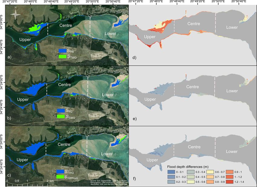
188                S. Kupfer et al.: Investigating the interaction of waves and river discharge during compound flooding

2020; Ward et al., 2017; Hendry et al., 2019; Wahl et al.,            The South African coastline comprises 291 estuaries, with
2015), as well as local-scale case studies distributed around      the majority of rapidly developing coastal towns situated
the globe (Mazas and Hamm, 2017; Bevacqua et al., 2019;            around estuaries (Hughes and Brundrit, 1995; van Niekerk
Klerk et al., 2015; Rueda et al., 2016), have drawn special at-    et al., 2020). Since estuaries are potentially prone to flooding
tention to statistical dependencies between flood drivers and      from fluvial and coastal high water levels, urban development
higher occurrence probabilities of compound events with cli-       in and around estuaries may be affected by compound flood-
mate change.                                                       ing (Pyle and Jacobs, 2016). For this reason, in 2019–2020,
   With climate-change-induced sea-level rise (Nerem et al.,       the South African Department for Forestry, Fisheries and En-
2018), potential changes in storminess (Church et al., 2013),      vironment conducted the National Coastal Climate Change
more extreme precipitation (Myhre et al., 2019), and higher        Assessment, which addressed coastal and estuarine flooding
river discharge (van Vliet et al., 2013), the risk of compound     (DEFF, 2020); however, this study did not account for com-
flooding is likely to increase, and flood extent, magnitude,       pound flooding.
and duration can be locally exacerbated (Couasnon et al.,             Flood impact assessments in general are rare, and those
2020).                                                             documented mostly assess the flood drivers individually
   Despite such studies focussing on dependencies between          (Fitchett et al., 2016; Mather and Stretch, 2012; Theron et al.,
flood drivers, little published research on compound flood         2010).
assessments exists, with most exploring the differences in            The main objective of this study is to analyse local-scale
flooding caused by the interaction of fluvial drivers with         compound flooding at Breede Estuary, a South African per-
storm surge and tides (e.g. Olbert et al., 2017; Kumbier et al.,   manently open estuary. Thereby we specifically account for
2018; Chen and Liu, 2014), pluvial drivers with surge (e.g.        the contribution of waves when they coincide with high river
Bilskie and Hagen, 2018; Bilskie et al., 2021), and tides (e.g.    discharge. In this context we assess the effects of compound
Shen et al., 2019). These studies successfully address the         flooding from river discharge, tides, and waves in terms of
driver interaction in hydrodynamic models and highlight the        magnitude and timing on the lower estuary by using the hy-
improved understanding of flood dynamics when consider-            drodynamic model Delft3D. We analyse the interaction of
ing the interaction of flood drivers (Olbert et al., 2017; Lee     all drivers and estimate the sensitivity of the flood charac-
et al., 2020; Shen et al., 2019; Seenath et al., 2016). When co-   teristics (extent, depth, and timing) to various driver combi-
inciding with high river discharge, the contribution of waves      nations and intensities. We chose Breede Estuary as it has a
to flooding is seldom addressed (e.g. Lee et al., 2020) even       large catchment and a notable tidal exchange, and data could
though waves play a substantial role in terms of flooding in       be obtained. Finally, the lower estuary has been shown to be
many of the discussed areas (Kumbier et al., 2018; Bilskie         prone to flooding from coastal and fluvial drivers (see Basson
and Hagen, 2018), while the influence on the timing of the         et al., 2017), and since we focus on the contribution of waves
flood has not been analysed in detail.                             during compound flooding, our study site is constrained to
   Waves can raise water levels (WLs) at the coast in terms        the lower estuary.
of wave set-up, which is described in detail by Dodet et al.          The paper is structured as follows. We describe the char-
(2019). Tanaka et al. (2009) have shown that in a shallow          acteristics of Breede Estuary in Sect. 2. We explain the hy-
and narrow estuary entrance, wave set-up can be up to 14 %         drodynamic model set-up, data used, and compound event
of the offshore wave height. For South Africa, Marcos et al.       scenarios in Sect. 3. In Sect. 4 we present flood characteris-
(2019) have shown a dependence of extreme WLs and waves,           tics resulting from the compound event scenarios, which we
and according to Melet et al. (2018) and Theron et al. (2010)      discuss in Sect. 5.
waves constitute the most important components of coastal
flooding for the country. Large destructive swells are gen-
erated by cold fronts, cut-off lows, and cyclones (Guastella       2   Study area
and Rossouw, 2012). These low-pressure systems cause addi-
tional heavy rainfalls, leading to immense fluvial flash floods    Of South Africa’s 291 estuaries, Breede Estuary is one of
(Pyle and Jacobs, 2016; Molekwa, 2013). Thus, a depen-             the largest permanently open estuaries (van Niekerk et al.,
dency between both drivers is likely. However, no published        2020). Breede River has the fourth largest annual runoff in
regional to local compound flood probability analyses exist        South Africa (Taljaard, 2003). It flows along 322 km from
for South Africa, and global statistical dependency analyses       the south-west of the country in a south-easterly direction to-
accounting for storm surge and river discharge only show           wards the South African south coast and enters the Indian
small correlations between drivers (Couasnon et al., 2020).        Ocean at the town of Witsand in Sebastian Bay (Fig. 1). The
This may be due to the fact that the surge contribution com-       estuary extends about 50 km upstream, where the tidal influ-
pared to other flood drivers, such as tides and waves, is rel-     ence ceases (Lamberth et al., 2008).
atively small in most South African estuaries (Theron et al.,         Breede Estuary is sparsely populated by small settlements
2010; Theron and Rossouw, 2008).                                   of up to 1000 inhabitants (e.g. Witsand; Fig. 1) situated
                                                                   on the northern and southern banks. The estuary provides

Nat. Hazards Earth Syst. Sci., 22, 187–205, 2022                                    https://doi.org/10.5194/nhess-22-187-2022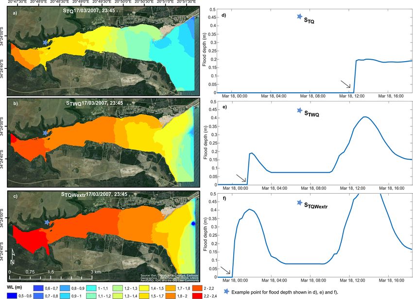
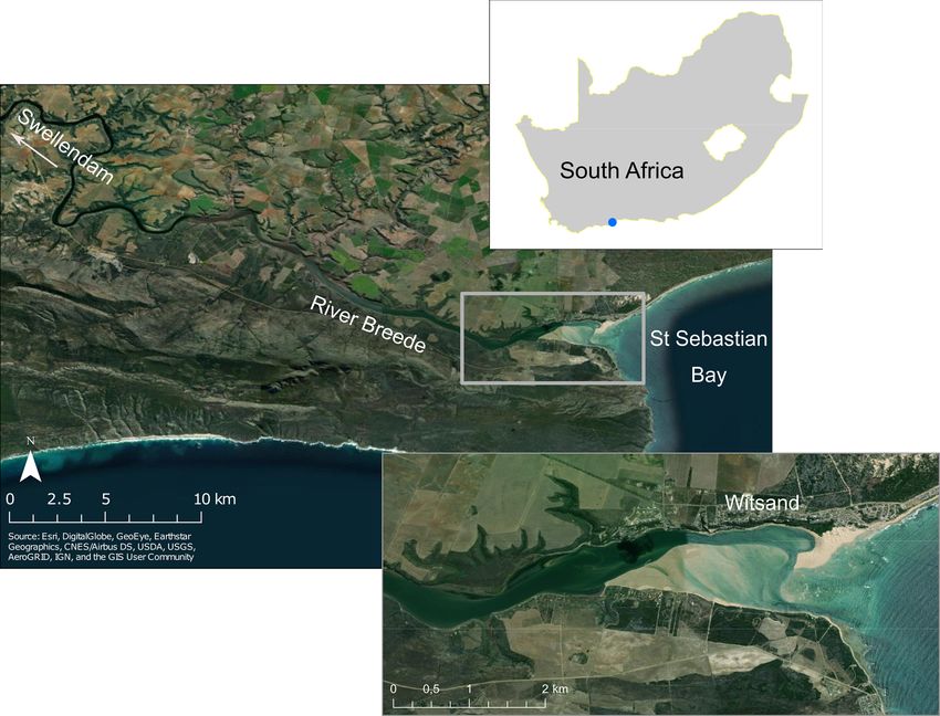
S. Kupfer et al.: Investigating the interaction of waves and river discharge during compound flooding                              189

Figure 1. Location of the study area and aerial photographs showing the Breede River and the Breede Estuary.

tourism services with several holiday resorts located along            treme WLs in South Africa (Melet et al., 2018). Such wave
the banks. Numerous farm properties spread along the banks             conditions are generated mainly by two synoptic weather
further upstream, and most of the land in the immediate sur-           systems, namely cold front systems and cut-off lows (Mather
roundings is privately owned agricultural land (SSI, 2016).            and Stretch, 2012). These are responsible for long-period
   Breede Estuary is open towards the south-east, where it             to local swell conditions, with waves approaching the south
enters the sea against a wave-cut terrace (Carter, 1983). Its          coast from south-westerly directions. Generally, annual mean
mouth is characterized by an open channel, which is located            significant wave heights (Hs ) range from 2.4–2.7 m (Basson
at the southern end of an extensive sand barrier formed by             et al., 2017). During extreme storm events significant wave
wave action (Schumann, 2013). Over the first 28 km, the                heights can reach more than 10 m, and peak periods (Tp )
depth of the estuary channel ranges from 3–6 m (SSI, 2016).            range from 5–20 s. The estuary mouth is relatively sheltered
At the lower estuary, the channel meanders along large and             from south-westerly waves since it is protected by a southern
shallow sand banks which have formed along the southern                headland of the bay (Fig. 1). Waves from the south-eastern
shore (Fig. 1).                                                        sector occur as well; however, these are generated by trop-
   During the low-flow summer months, the estuary is marine            ical cyclones, making landfall at the Mozambican and the
dominated, meaning the estuary receives high seawater input            South African east coast (DEA&DP, 2012). The dominat-
(SSI, 2016). Due to the relatively strong tidal inflow during          ing wind direction is from the westerly and easterly sector,
summer (Taljaard, 2003) and the sand barrier restricting the           whereby easterly winds generate local wind waves penetrat-
estuarine inlet, the estuary can be classified as tide and wave        ing into the estuary as its opening faces east (Vonkeman et al.,
dominated (Cooper, 2001).                                              2019). One example of coastal flooding occurring in the area
   The main tidal signal is semi-diurnal (M2), with addi-              was an extreme storm in August 2008. Waves of 10.7 m were
tional diurnal oscillations (Schumann, 2013). During spring            measured, and since the storm lasted longer than 12 h, the
tidal periods, the tidal range can reach up to 2 m, as mea-            extreme waves additionally co-occurred with high tide levels
sured at the tide gauge of Witsand, situated at the northern           1 d after a spring tide. Consequently, a large area of the South
shore of Breede Estuary (Fig. 1). The southern coastline is            African south coast was affected, resulting in severe damage
wave dominated and experiences the highest wave conditions             to coastal infrastructure (Guastella and Rossouw, 2012).
along the entire South African coast (Theron et al., 2010).               During winter, the estuary is highly responsive to freshwa-
Thus, waves cause the largest relevant contribution to ex-             ter inflows (Taljaard, 2003). The catchment receives 80 % of

https://doi.org/10.5194/nhess-22-187-2022                                        Nat. Hazards Earth Syst. Sci., 22, 187–205, 2022
190 S. Kupfer et al.: Investigating the interaction of waves and river discharge during compound flooding
Table 1. Datasets and characteristics applied to set up Delft3D.
Dataset Source Horizontal Temporal Time period Reference
resolution resolution system
Bathymetry Basson et al. (2017) 5m – – MSLa
Elevation SUDEM van Niekerk (2016) 5m – – MSL
Land cover, bottom roughness DEA (2015)b 30 m – – –
Tides FES2014 AVISO (2014) 1/16◦ 1h 1980–2014 MSL
Q H7H006 (DWS) – 1h 1966–2019 Local MSL
Waves Basson et al. (2017) – Constant – –
Observations H14T007 (DWS) – 1h 2002–2019 Local MSL
a Mean sea level (MSL); b Kaiser et al. (2011), Jung et al. (2011), Wamsley et al. (2009), Mourato et al. (2017), Chow (1959).
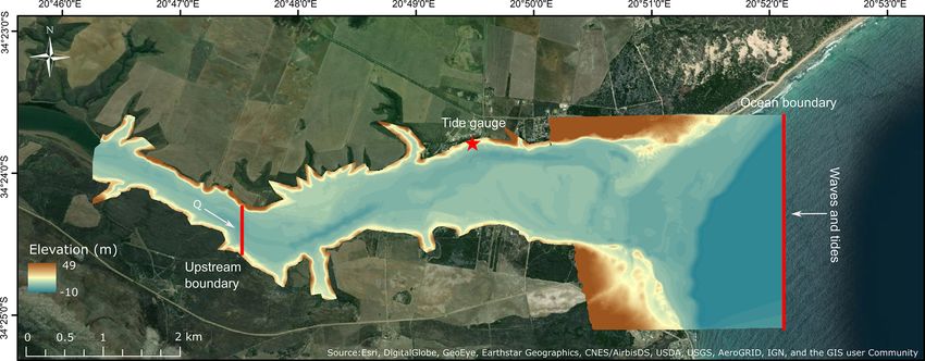
Figure 2. Model domain, including the merged bathymetry and elevation raster, the location of the Witsand tide gauge, and the two open
boundaries.
the annual rainfall during winter months, causing peak flows hereafter referred to as Q. We used the hydrodynamic nu-
and floods usually during that season. Breede Estuary has merical module Delft3D-FLOW, coupled with the module
experienced extreme fluvial flooding, with major events oc- Delft3D-WAVE, which is based on the SWAN (Simulate
curring in 1906, 2003 and 2008. In November 2008, intense Waves Nearshore) model.
rainfall far upstream, caused by a cut-off low, resulted in ex- Setting up a hydrodynamic model requires numerous in-
treme river runoff (Holloway et al., 2010). Extreme river dis- put datasets. The characteristics of the datasets used in this
charge caused WLs up to 10 m in the upper 20 km of the study are shown in Table 1. A detailed description of the pre-
estuary while levels of 50 cm were measured at the estuary processing of the datasets used as Delft3D input files and the
entrance (Basson et al., 2017). A similar cut-off low event model set-up is provided in Appendix A.
occurred in May 2021 but was less extreme, with estimated We performed simulations using tides and Q as input
elevated WLs being 1–2 m in the upper reaches. data in Delft3D-FLOW on a 5 m × 5 m rectangular grid in
a depth-averaged (2D) mode for the model validation, as
well as scenario runs. The 2D mode has been successfully
3 Methods applied in numerous hydrodynamic flood modelling studies
(Kumbier et al., 2018; Skinner et al., 2015; Olbert et al.,
3.1 Hydrodynamic model and data description 2017). As we focus on the additional contribution of waves
during compound flooding, the model domain is restricted
We used the fully integrated open-source modelling suite
to the lower estuary (Fig. 2). Topographic input data were
Delft3D (Lesser et al., 2004) which has been extensively
merged with bathymetric data, which were manually digi-
used in coastal applications (Lyddon et al., 2018; Bastidas
tized, based on a bathymetry of an existing study report on
et al., 2016; Kumbier et al., 2018) for simulating flood ex-
flood lines at the Breede Estuary (Basson et al., 2017). We
tents and flood depths from waves, tides, and river discharge,
Nat. Hazards Earth Syst. Sci., 22, 187–205, 2022 https://doi.org/10.5194/nhess-22-187-2022
S. Kupfer et al.: Investigating the interaction of waves and river discharge during compound flooding                                 191

Table 2. Tidal events used for validation and dates of occurrence.

                         Event name        Average            Neap               Spring              Spring + high Q
                         Date              14–19 Jul 2007     18–23 Sep 2007     27 Sep–1 Oct 2007   22–25 Nov 2007

Table 3. Scenario descriptions.                                            tion and validation since no measured nearshore wave time
                                                                           series could be obtained.
  Scenario    River discharge     Tide       Waves                            For the validation, we performed three simulations cov-
  STQ         100-year            Spring     –                             ering the full tidal range and compared the model output to
  STW         100-year            Spring     100-year (ESE direction)      the corresponding observed WLs (Matte et al., 2017; Muis
  STWQ        100-year            Spring     100-year (ESE direction)      et al., 2017). To account for the full tidal range, these simu-
  STQWextr    100-year            Spring     100-year (all directions)     lations include a spring, average, and a neap tide event (see
                                                                           Table 3 for the event names and dates of occurrence). For
                                                                           these simulations we selected events in which Q was con-
                                                                           stantly low in order to focus on model performance when
specified spatially varying manning bottom roughness via lit-
                                                                           the model is driven only from the ocean boundary and where
erature review from gridded land cover data (Table 1). We ob-
                                                                           continuous observations exist. To test the performance of the
tained 17 years of hourly measured WL observations serving
                                                                           model when driven by both the oceanic and the upstream
for the model calibration and validation from the tide gauge
                                                                           river boundary, we selected the largest continuously recorded
station H14T007 (DWS, 2020a), located in the small harbour
                                                                           high Q event occurring within the period of observed WLs
of the town of Witsand (Fig. 2).
                                                                           at the tide gauge in Witsand (Table 2).
   We forced the model at two open boundaries. The ocean
                                                                              According to the tide gauge data, this high Q event
boundary (Fig. 2) is located at the westernmost edge of the
                                                                           (1262.78 m3 s−1 ) occurred simultaneously with a relatively
model domain and perpendicular to the main flow direction.
                                                                           large tidal range of up to 1.6 m. For this event the time lag
Depending on the scenario, we forced this open boundary
                                                                           of Q reaching the upstream open boundary from the mea-
with tides and waves. We used historical tidal input data (Ta-
                                                                           suring station must be considered. Thus, we estimated the
ble 1) which were obtained from the global tidal FES2014
                                                                           difference between the timing of the peak from the upstream
model (AVISO, 2014; Carrère et al., 2015). The data were
                                                                           flow gauge and from the non-tidal residual (NTR; see Ap-
extracted at a point closest to but still located 24 km offshore
                                                                           pendix C) of the tide gauge, whereby we considered the max-
from the westernmost edge of the model domain (Fig. 2).
                                                                           imum WL as the peak, caused by Q, since the tidal phase at
The second boundary (upstream boundary; Fig. 2) is situated
                                                                           this stage was at low tide level. We estimated a time lag of
at the upstream border of the model domain, perpendicular to
                                                                           8 h, with the peak at the tide gauge occurring later (Fig. D3).
the river flow, and was forced by hourly measured Q from the
                                                                           We accounted for this time lag in the Q boundary conditions
station in Swellendam (Table 1), which was the closest to the
                                                                           for the validation run to enable the comparison of model out-
upstream boundary (54 km). For the Delft3D-WAVE set-up,
                                                                           put and tide gauge data.
we increased the grid cell size and the horizontal resolution
of the input bathymetry to 10 m for computational reasons.
Since nearshore wave time series could not be obtained, a                  3.3    Event selection and scenario development
constant sea state (constant Hs and constant Tp ) serves as
wave boundary conditions (ocean boundary; Fig. 2) which                    To assess compound flooding in terms of magnitude and
we obtained from two extreme value analyses (EVAs) per-                    timing, we developed four scenarios, accounting for tides,
formed by Basson et al. (2017).                                            waves, and Q. Storm surge was not considered as no
                                                                           nearshore WL time series could be obtained, and offshore
3.2   Model calibration and validation                                     input data would even increase model uncertainties. Addi-
                                                                           tionally, analysis of tide gauge data along the South African
To evaluate the performance of the model, we calculated the                coastline has shown that at the South African south coast
goodness-of-fit parameters R 2 (coefficient of determination),             storm surge makes a small contribution, relative to the other
the Pearson correlation, r, and the root mean square error                 considered flood drivers, even when considering extreme
(RMSE) between the model output and observed WL time                       surges such as a 100-year event (Theron and Rossouw, 2008;
series (see Skinner et al., 2015). During model calibration,               Theron et al., 2014). Moreover, Melet et al. (2018) showed
we adjusted the bottom roughness and horizontal eddy vis-                  that the wave contribution to extreme WLs in South Africa
cosity (see Appendix A). We used the best-fitting physical                 is substantially larger compared to the surge contribution. To
parameters to set up the model for model validation and the                explore this further, we additionally estimated the NTR of
scenario runs. Waves were excluded during model calibra-                   the tide gauge data of Witsand, which showed that the mean

https://doi.org/10.5194/nhess-22-187-2022                                             Nat. Hazards Earth Syst. Sci., 22, 187–205, 2022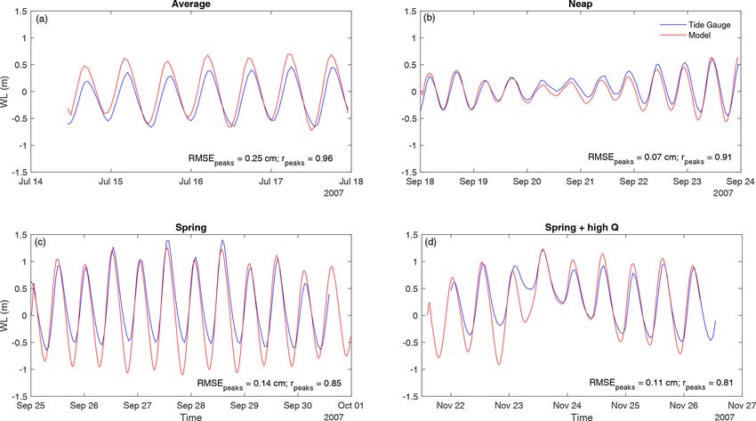
192               S. Kupfer et al.: Investigating the interaction of waves and river discharge during compound flooding

amplitude of the NTR of 10 cm is small compared to the           et al., 2017). To compare the results of the WL scenarios,
tidal range of 2 m (Fig. D1). The contribution of wave set-      flood extents and flood depths were extracted at the time of
up and Q is still included in the NTR, and large peaks could     the maximum flood.
be identified as being caused by Q (see Fig. D2 and more in-
formation on the analysis in Appendix D). To investigate the
effects of Q and waves on the flood characteristics during       4     Results
compound flooding, we developed the following scenarios
                                                                 4.1    Model validation
(Table 3).
   The scenarios were named according to their driving           For all validation runs the model set-up was able to reproduce
mechanisms. Thereby T stands for tides, W for waves, and         the timing of flood and ebb tide (Fig. 3). Variations occurred
Q for river discharge. The selected extremes were extracted      however in the WL magnitude, especially during the average
either via peak-over-threshold (POT) analysis or by finding      event at high tide (Fig. 3a), where simulated WLs were 25 cm
the maxima in the time series. All scenarios assume that the     higher than the observed for average tidal conditions. During
peaks of the drivers occur at the same time (Harrison et al.,    low tide events in the spring tide simulation, modelled WLs
2021). The maximum Q event within the hourly time se-            were up to 60 cm lower (Fig. 3c), and peak values only, how-
ries applied for this study has a peak value of 1357 m3 s−1      ever, showed differences of maximum 14 cm (see RMSE Ta-
and occurred in November 2008. According to Basson et al.        ble C1). The neap tide event on the other hand was simulated
(2017) this value was corrected to 1546 m3 s−1 , correspond-     with a RMSE of only 10 cm (Fig. 3b) and peak values of only
ing to a return period of 15 years. The value was corrected      7 cm (Table C1). The goodness-of-fit estimates also showed
as for this event the flow gauging station stopped measuring     agreement of observed and modelled WLs for all tidal events
before the peak was reached. Based on this value, a peak Q       excluding Q (Table C1).
of 3295 m3 s−1 corresponds to a 100-year event which we se-         Moreover, for the simulation that included high Q
lected here as extreme Q (see Basson et al., 2017, for a more    (Fig. 3d) the compared maximum WL peak did not show
detailed description). We developed the Q hydrograph to          any difference. After the maximum event peak, however, the
force the upstream open boundary by normalizing the hydro-       model overestimated flood peaks by up to about 30 cm. WLs
graph of the highest Q event for which the full hydrograph       during low tide before the peak of the event were strongly
was available. We then multiplied the normalized hydrograph      underestimated (∼ 70 cm) by the model. The goodness of fit,
with the 100-year peak value. For the STW , so the no-Q sce-     however, did not differ much from tide-only conditions (Ta-
nario, we kept the upstream boundary open so that incoming       ble C1). As flooding is usually caused by peak WLs and sim-
flood water does not accumulate there. Thus, we chose the        ulated peaks showed an RMSE of 0.15 m compared to ob-
lowest measured Q event from the time series, where Q does       servations for all validation runs, we considered the model
not exceed 1.2 m3 s−1 . For the spring tide event, we selected   performance as fit for purpose.
the maximum tidal flood peak of 1.3 m from the FES2014
tidal input data, which occurred in March 2007.                  4.2    Flood sensitivity to varying driver combinations
   For the wave conditions, we chose two 100-year wave
events from two different extreme value analyses (EVAs) of       To analyse the scenario results according to their flood char-
Basson et al. (2017). According to their EVA, a 100-year         acteristics in terms of magnitude and timing and to estimate
wave event coming from east-south-easterly (ESE) directions      the wave contribution, we initially compared the compound
(110◦ ), the direction from which waves directly penetrate the   flood scenario STWQ to scenarios in which one driver was ex-
estuary, has an Hs of 6.2 m and a Tp of 12 s. To consider        cluded (STW , STQ ). Then we compared the compound flood
an even higher wave event for a final worst-case scenario,       scenario STWQ with the extreme wave compound flood sce-
Hs was increased to 9.3 m and Tp to 19.95 s, correspond-         nario (STQWextr ). WLs, flood extent, and maximum and mean
ing to Hs and Tp of a 100-year wave event when consider-         flood depths of all compound scenarios are summarized in
ing all wave directions in the EVA. The ESE wave direction       Table E1 of Appendix E. For demonstrative reasons we sep-
was maintained for all scenarios that include waves. For the     arated the model domain into three areas, termed “upper”,
sea states driving the model, it must be pointed out that Bas-   “centre”, and “lower” domains, as shown in Fig. 5.
son et al. (2017) performed EVAs on offshore wave data. As          The results of the compound flood simulation (STWQ ) with
the location of the open boundary for this study is located      the simulation excluding river discharge (STW ) showed large
nearshore, the considered wave scenarios may be more ex-         differences in all flood characteristics. The WLs of STWQ
treme than the sea state would be at the open boundary as        were substantially higher throughout the entire estuary than
wave refraction and diffraction were not accounted for. Due      the WLs produced by accounting only for oceanic drivers
to computational constraints and data limitations, we have       (STW ; Fig. 4). The WLs of STW showed a continuous state
employed the 100-year return period for waves and Q as this      around 1.54 m throughout the entire estuary, slightly decreas-
was also recommended by previous flood assessment studies        ing towards the estuary mouth. As in STWQ , WLs were high-
for South Africa (e.g. Theron and Rossouw, 2008; Basson          est at the upstream open boundary and decreased substan-

Nat. Hazards Earth Syst. Sci., 22, 187–205, 2022                                 https://doi.org/10.5194/nhess-22-187-2022
S. Kupfer et al.: Investigating the interaction of waves and river discharge during compound flooding                                 193

Figure 3. WLs of the model validation runs (red curve) at the tide gauge station compared to observed WLs from the tide gauge (blue curve).
Panel (a) shows WLs of the average tide event, (b) the neap tide event, (c) the spring tide event, and (d) the high river discharge event,
coinciding with the spring high tide. All panels include goodness-of-fit estimates for peak values of each event (RMSEpeaks , rpeaks ).

                                                                        tially towards the estuary mouth, and the largest WL differ-
                                                                        ences between both scenarios occurred at the upper domain
                                                                        with up to 1.5 m. Further towards the estuary mouth differ-
                                                                        ences reached a minimum of 15 cm, decreasing towards the
                                                                        outside area.
                                                                           Figure 5a presents the flood extent of STW on top of the
                                                                        extent of STWQ , which showed a substantially larger extent.
                                                                        Further, both scenarios showed large spatial differences in
                                                                        flood extent patterns. STWQ inundated an additional extent
                                                                        of 45 % compared to the flood produced by the STW scenario
                                                                        (Table D1). During the compound scenario, the flood covered
                                                                        a large low-lying area at the northern shore (about 5 km from
                                                                        the mouth), inundating up to 570 m further inland. However,
                                                                        in the scenario STW in which Q was excluded, only a narrow
                                                                        area got flooded, reaching at its widest part 250 m inland.
                                                                        On the southern bank (centre), the STWQ flood reached 80 m
                                                                        further inland than STW . At the estuary mouth, both scenarios
                                                                        flooded about the same areas.
                                                                           Figure 5b represents differences in flood depths. From the
                                                                        estuary mouth towards the estuary entrance, differences in
                                                                        flood depths showed the same pattern as differences in WLs.
Figure 4. WL (m) with distance from the upstream boundary of all        At the sand barrier, flood depth differences reached up to 1 m.
scenarios, with the vertical dashed line demonstrating the location        Comparing WLs of the Q scenario in which waves
of the estuary mouth. The map shows the location of the transect        were excluded (STQ ) to the compound flood scenario STWQ
(yellow line), as well as the location of the upstream open boundary
                                                                        (Fig. 4), both WL curves showed the same pattern, with the
(vertical orange line) and the estuary mouth (dashed grey line).
                                                                        WLs of STWQ generally being higher than those simulated
                                                                        by STQ . The differences in WLs between both scenarios de-
                                                                        creased from the area around the estuary mouth with max-

https://doi.org/10.5194/nhess-22-187-2022                                         Nat. Hazards Earth Syst. Sci., 22, 187–205, 2022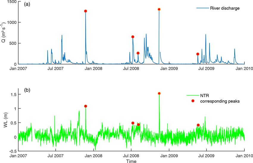
194                S. Kupfer et al.: Investigating the interaction of waves and river discharge during compound flooding

Figure 5. Comparison of flood extents of compound scenario and that excluding the driver (a–c) and differences in flood depths (d–f).
Panel (d) shows the flood depths of STWQ -STW , (e) shows STWQ -STQ , and (f) shows STQWextr -STWQ .

imum differences of 53 cm towards the centre of the study            towards the estuary entrance. Such differences are further en-
area. We found the smallest differences of ∼ 20 cm close to          countered in the flood depth, showing the same magnitude
the upstream edge of the model domain where WLs were                 in the entire lower area. Generally, the higher flood depths
highest in both scenarios. We observed a similar pattern in          produced by STQWextr reached towards the upstream open
flood depth differences (Fig. 5e), showing a maximum of              boundary, but the differences were decreasing (Fig. 5f). The
70 cm at the northern shore of the estuary entrance, decreas-        flood extent was 12 % larger when considering large waves
ing towards the upstream boundary to ∼ 20 cm. Figure 5b              during compound flooding. Spatially, the larger flood plain
shows the overlaying flood extents of both scenarios, where          in STQWextr was mainly restricted to the southern shore of the
both scenarios inundated mostly the same areas. The flood            central and lower model domain. In these areas, the STQWextr
extent of STWQ covered a 10 % larger area than the flood re-         extent expanded up to 40 m further inland than the extent of
sulting from STQ (see Table D1 for the flood size). Inside the       STWQ . At the northern shore, the only noticeable area which
estuary, the largest differences occurred in the populated area      got flooded in STQWextr , but not in STWQ , was the sand barrier
at the southern shore (centre).                                      forming the estuary mouth. STQWextr almost entirely flooded
   As anticipated, both scenarios accounting for all three           the sand dune, indicating that it is likely to be eroded during
drivers during an extreme stage (STWQ and STQWextr ) showed          a flood (Fig. 5c).
the highest values in terms of inundation depth and extent.             To further estimate the effects of waves during compound
Comparing the compound flood scenario (STWQ ), with the              flooding on the timing of the flood, different time steps of
one including even higher extreme waves (STQWextr ), we              the flood WLs in scenarios STQWextr , STWQ , and STQ are pre-
found large differences in the WLs throughout the entire             sented in Fig. 6. Figure 6a–c show all three scenarios at the
study area (Fig. 4).                                                 same time step (17 March 2007, 23:45 GMT+2; all times are
   Inside the estuary, STQWextr produced continuously higher         GMT+2), which was selected according to the onset of high
WLs than STWQ , with increasing differences of up to 40 cm           WLs at the upstream open boundary in STQ . The three sce-

Nat. Hazards Earth Syst. Sci., 22, 187–205, 2022                                      https://doi.org/10.5194/nhess-22-187-2022

S. Kupfer et al.: Investigating the interaction of waves and river discharge during compound flooding                                    195

Figure 6. WLs of the scenarios STQ , STWQ , and STQWextr , extracted at the same time step (a–c) and time series of all three scenarios (d–f),
showing the timing of the onset of the flood extracted from the point marked by the blue star.

narios at the same time step showed the highest WLs at the               5     Discussion
upper model domain, which then decreased towards the open
sea. Generally, STQ produced the lowest WLs (Fig. 6a), fol-              5.1    Effects of interaction between drivers during
lowed by STWQ (Fig. 6b), and the largest WLs were produced                      compound flooding and the contribution of extreme
in STQWextr (Fig. 6c).                                                          waves
   The figure also reveals differences in the areas in which the
high WLs dominated at that time. While in STQ WLs of up                  Model outputs show differences in the magnitude of and
to 1.8 m were only shown in the upper area, the same magni-              spatial variation in flood characteristics between all scenar-
tude of WLs reached until 4.2 km in STQW and even crossed                ios. Spatial variations in flood characteristics of the dif-
the estuary mouth in STQWextr . Furthermore, Fig. 6d–f show              ferent scenarios indicate locations where the interaction of
the timing of the onset of the flood in the three scenarios at           waves, tides, and Q during compound flooding have am-
the point highlighted by the blue star, shown in Fig. 6a–c.              plified flooding and where individual drivers contribute to
In STQWextr the area got flooded earliest (18 March at 00:00;            the flood. Enhanced flood characteristics during compound
Fig. 6f) and was followed 90 min later by STQW (Fig. 6e). In             flooding and spatial variations in the flood pattern caused
STQ , however, the same area got flooded even 12 h later on              by different driver combinations were previously discussed
18 March at 12:00.                                                       by Olbert et al. (2017), Kumbier et al. (2018), and Harrison
                                                                         et al. (2021), as well as by Bilskie and Hagen (2018). Yet,
                                                                         none of the studies accounted for the additional influence of
                                                                         waves. In addition to this, none of them addressed the effects
                                                                         of the oceanic flood drivers on the timing of the flood when
                                                                         co-occurring with Q.

https://doi.org/10.5194/nhess-22-187-2022                                           Nat. Hazards Earth Syst. Sci., 22, 187–205, 2022
196 S. Kupfer et al.: Investigating the interaction of waves and river discharge during compound flooding The comparison of STWQ with the riverine (STQ ) and the pound flooding, which was not apparent when considering wave scenario (STW ) highlights that compound flooding in- the components individually. High outflowing Q can also creases flood extent and depth. In particular, the additional dampen the wave and tidal propagation inside the estuary, extent in the central study area, as well as the continuously causing increased WLs at the entrance (Sassi and Hoitink, higher WLs and water depths during compound flooding 2013). This implies that during compound flooding, waves (Fig. 5a–d), indicates an accumulation of water inside the play a stronger role when coinciding with Q by amplifying estuary. the flood magnitude. When considering flood drivers individ- The results further reveal where each driver has its high- ually, however, the effects caused by waves were relatively est influence. This information is relevant for understanding low, as compared to effects caused by Q. the flood dynamics due to driver interaction and the wave We further assessed the wave contribution by testing the contribution. Regions only inundated in the compound flood sensitivity of compound flooding to more extreme wave con- scenario but not in STW or STQ were mostly located in the ditions. Comparing results of the compound flood scenario central zone of the study area. In STWQ additional inundated STWQ with results of the extreme wave compound flood areas in the upper sector were small (10 %) when compared (STQWextr ) confirms the expected larger flooding caused by to STQ but were large (45 %) when compared to STW . These more intense waves. This was valid for all flood character- floods highlight the generally higher effect of river discharge istics throughout the entire study area. The effects of in- in the more confined upper section during compound flood- creased wave conditions were found to be greatest in the ing. The influence of Q decreases towards the mouth area lower reaches. First, the considerably larger flood extent at as increased friction through the widening of the estuary at the sand barrier can be explained by wave overtopping and the central area and the large flood plain at the upper north- shows that extreme wave conditions coinciding with spring ern shore of the domain attenuate the flood wave (Cai et al., high tides may lead to eroding and a breaching of the bar- 2016). In contrast, waves have clearly been shown to be the rier. As explained above, wave set-up can raise WLs inside dominating factor at the estuary mouth area, resulting in sub- the estuary (Olabarrieta et al., 2011), which becomes more stantially higher WLs (Fig. 4). These can be caused by wave extreme with higher waves. An impact of waves on WL set-up as the steep bathymetry and shallow water depths out- variabilities in South African estuaries has previously been side the estuary cause waves to break before entering (Carter, shown by Schumann (2013) who states that waves together 1983; Xu et al., 2020), increasing WLs inside the estuary. with the tidal influence can determine how far ocean wa- Tanaka et al. (2009) have shown that in a shallow and nar- ter propagates upstream in an estuary. Therefore, increased row estuary entrance, wave set-up can be up to 14 % of the wave conditions during compound flooding do not only have offshore wave height, which strongly depends on the mor- effects on the lower domain flood extent and depth. STQWextr - phology of the inlet. Olabarrieta et al. (2011) demonstrated enhanced flood characteristics in the upper domain, as shown that wave set-up propagates inside the estuary and interacts in all STQWextr -related figures (Figs. 4, 5c and f, and 6c and f), with outflowing currents (Olabarrieta et al., 2011; Zaki et al., confirm the fact that higher waves cause greater impacts fur- 2015). Additionally, the funnelling effect due to the narrow ther upstream when compared to STWQ . estuary mouth may amplify wave-set-up-induced WLs (Lyd- Last, an interesting finding of the study is that compound don et al., 2018), contributing to the elevated WLs inside the events do not only affect flood characteristics in terms of estuary and causing a relatively large flood extent at the sand magnitude. barrier in STW . The small differences in flood characteristics The timing of the flood also changed when all drivers co- in the upper area (STWQ vs. STQ ), however, demonstrate a incide and when stronger wave conditions are accounted for. decreasing influence of waves from the entrance towards the The increased volumes of water during the compound event upstream boundary of the model domain. and in STQWextr resulted in flooding occurring earlier than In STWQ the increased WLs at the entrance and the larger when the drivers, waves, and Q were not coinciding. Figure 6 flood extents at the sand barrier and in the central estuary shows that at the specific considered time step, the flood char- indicate an interaction of drivers mostly in the lower area. acteristics of STQWextr were largest (also in the upper area), Delpey et al. (2014) have shown that extreme waves can although at that time Q was still moderate. Therefore, even reduce the freshwater outflow from the estuary mouth to- when the riverine component was still moderate, waves led wards the open ocean, increasing the water volume inside to enhanced flooding. Considering the timing at which most the estuary, and thereby raise the WLs. Such a blocking of of the flood plain marked in Fig. 6 was inundated in all three the riverine component through the oceanic component was scenarios (see Fig. 6d–f) further highlights the large wave also observed in Orton et al. (2020), although they only ac- contribution during compound flooding. In this case the flood counted for tides and excluded waves. Hence, the blocking plain was flooded earliest in STQWextr , followed by STWQ of Q through waves may explain the larger flood character- about 95 min later. When not accounting for waves, however, istics in STWQ at the central domain area, even approximat- the flood plain was inundated 12 h later than in STWQ . These ing the upstream open-model boundary. This shows a large findings indicate that waves play a substantial role when co- contribution of waves to flood characteristics during com- inciding with the fluvial component and spring tides as they Nat. Hazards Earth Syst. Sci., 22, 187–205, 2022 https://doi.org/10.5194/nhess-22-187-2022
S. Kupfer et al.: Investigating the interaction of waves and river discharge during compound flooding                         197

lead to larger flooding and an earlier onset of the inundation,   model. Thus, the higher observed WLs could have been pro-
even when Q was still moderate.                                   duced by wave set-up or less likely a storm surge (Zaki et al.,
                                                                  2015). Relative to other flood drivers, storm surge alone does
5.2   Model performance, limitations, and outlook                 not have a significant effect on coastal flooding along the
                                                                  South African south and west coasts (Theron et al., 2014),
This analysis has shown the sensitivity of flood character-       but it still may affect WLs inside the estuary (Lyddon et al.,
istics to compound flooding when compared to individual           2018). Testing the effect of waves and surge on the model
flood drivers. This was demonstrated by spatial variabilities     performance, however, would require observed wave time se-
in the flood extents and by variabilities in the flood magni-     ries and nearshore WL data which were not available for this
tude and timing. We must note, however, that flood extent         study.
and depths could not be directly validated. Commonly used            Storm surge has been considered in most regional or local
data types for flood impact validation are pictures, satellite    flood assessments, specifically in those dealing with com-
imagery, and high watermarks (Molinari et al., 2017). Yet,        pound flooding (Eilander et al., 2020; Olbert et al., 2017;
such data were not available for the study area. According        Shen et al., 2019). Despite its low contribution at the lo-
to Basson et al. (2017), pictures and high watermarks of a        cation of Breede Estuary (Appendix C), storm surge may
fluvial flood occurring in 2008 exist, however, only at sites     still contribute to compounding drivers to become an ex-
further upstream. This area was not considered in the model       treme event, even when neither of the drivers is extreme
domain of this study as detailed upstream bathymetry data         (Leonard et al., 2014). To estimate its contribution, storm
could not be obtained. Nevertheless, model performance was        surge should be considered in further simulations. Our anal-
validated at the tide gauge at Witsand near the mouth (Fig. 2).   ysis presents driver interactions during extreme (100-year)
Flood peaks matched the observed peaks in almost all sim-         conditions without showing joint probabilities of waves
ulations (Fig. 3, Table C1). The model overestimated tidal        and Q. Further, we assumed that maximum flooding occurs
high-water peaks only during the average tide event. Tidal        when all drivers peak simultaneously and did not account for
low water peaks, though, were generally underestimated.           differences in the relative timing of all driver peaks. How-
   Those differences can be explained by uncertainties inher-     ever, Harrison et al. (2021) conducted such a sensitivity anal-
ent in the model input data, such as tides and bathymetry.        ysis and found that the effect of the timing of driver peaks
Tides, serving as input data for model validation and all sce-    strongly depended on estuary size. They also found that in an
narios of this study, were obtained from the global FES2014       estuary comparable in size to Breede Estuary this effect was
tidal model (Carrère et al., 2015). Even though the model         negligible. However, as estuaries can also differ in aspects
shows a rather high accuracy offshore, on shelves, and on         other than size (e.g. morphological characteristics), assessing
nearshore areas (Stammer et al., 2014; Ray et al., 2019), the     the effect of the timing of the driver peaks could provide fur-
local-scale coastal processes caused by the local topography      ther insights on the flood mechanisms of compound flooding.
and the influence of the estuarine channel morphology (Wang       This information, together with information on joint prob-
et al., 2019; Godin and Martínez, 1994) are not considered in     abilities, becomes relevant when assessing risk from com-
the data. Additionally, the model open boundary was placed        pound flooding, which is beyond the scope of this study and
at a location several kilometres further nearshore of the point   should be considered in future work. For such a risk assess-
from which the tidal inputs were extracted. Processes mod-        ment a wider range of return periods should also be explored.
ifying the tidal propagation between both locations were
therefore not considered. One way to overcome this limita-
tion would be to downscale the tides from the model towards       6   Conclusions
the location of the open boundary, which, however, is beyond
the scope of this study. Moreover, permanently opened estu-       We assessed compound flooding from tides, Q, and waves at
aries are highly dynamic areas due to a constant influence        the permanently open Breede Estuary (South Africa) using a
of sediment deposition by river inflow and sediment removal       hydrodynamic model. For the assessment, we simulated sce-
due to floods (Moore et al., 2009; Whitfield et al., 2012). The   narios accounting for the three flood drivers (i.e. tides, Q, and
sand bars and sand banks at the timing of the validation runs     waves) and scenarios omitting either waves or Q in order to
(covering events in 2007) were therefore likely in a differ-      analyse their contribution. We found that flood characteris-
ent position than at the time when the input bathymetry was       tics such as extent, water depth, and timing are affected by
generated (Basson et el., 2017). This can have a high im-         the interaction between the drivers. As anticipated, the omis-
pact on water levels at the location of the tide gauge (Wang      sion of waves caused major inundations to occur in the upper
et al., 2019). Additionally, the omitted storm surge, wind, and   domain area, whereas the omission of Q produced compa-
waves as model input during the validation runs can explain       rably small flooding. Thus, we have shown that when con-
the large discrepancies occurring specifically in the Q vali-     sidered separately, the contribution of waves to flooding was
dation run (Fig. 3d), in which tidal low water peaks preced-      small. When waves were combined with spring tides and Q,
ing the actual event peak were strongly underestimated in the     however, they had a substantial effect on the spatial distribu-

https://doi.org/10.5194/nhess-22-187-2022                                  Nat. Hazards Earth Syst. Sci., 22, 187–205, 2022
198 S. Kupfer et al.: Investigating the interaction of waves and river discharge during compound flooding
tion and magnitude of the floods by impeding river flow to a period of 53 years, from 1966 until 2019. Hourly water
the sea. A notable impact of waves during compound flood- level observations serving for the model calibration and val-
ing was their effect on the flood timing. Through backwater idation were provided by the DWS from the tide gauge sta-
effects, waves induced the flood to occur earlier. This was tion H14T007 (DWS, 2020a), located in a small harbour of
further emphasized when increasing the wave intensity in the town of Witsand inside the estuary mouth. The measure-
the compound flood scenario. We therefore suggest that com- ments cover 17 years (2002–2019). We derived wave data,
pound flooding induced by high Q, tides, and waves should significant wave height (Hs ), and peak period (Tp ) from two
not only be considered in risk assessment studies in terms of extreme value analyses (EVAs) performed by Basson et al.
magnitude but also in terms of timing. The earlier onset of (2017). They extracted from the ECMWF model simulated
intense flooding needs to be accounted for when forecasting, offshore wave data of 37 years (1979–2016), from a point
planning, and managing flood hazards. close to the estuary, while still being located 30 km off the
As we have shown in this study for Breede Estuary, com- coast.
pound flooding can exacerbate flooding, and waves make
a substantial contribution to flooding when coinciding with
extreme Q. Extreme waves co-occurring with spring tides Appendix B: Model set-up and model calibration
and high precipitation have been documented by Guastella
Grid and topography of the model are based on the Cartesian
and Rossouw (2012), who additionally predicted a change
coordinate system WGS84/UTM zone 34S. The model do-
in wave climate for the South African south-west coast to-
main expands over an area of 19.2 km2 , covering the lower
wards more frequent extreme wave conditions. Our results
estuary and the area until 1.5 km offshore (Fig. 2). We used
in combination with a changing wave climate further con-
a time step of 1.5 s for calibration, validation, and scenario
firm the necessity of accounting for compound flooding and
runs, as was suggested by the Courant number. We changed
specifically waves in future local flood impact assessments in
the reflection parameter α, which determined the permeabil-
South Africa, particularly for other South African estuaries,
ity of the open boundaries to 1000 for the ocean boundary
which are highly populated, like Umgeni Estuary (Durban),
and to 200 for the upstream boundary, as the model oth-
Swartkops Estuary (Port Elizabeth), Nahoon Estuary (East
erwise produced instabilities in preliminary runs (Deltares,
London), and Diep Estuary (Cape Town), where it can lead to
2014a). Additionally, we considered several physical and nu-
substantial infrastructure damage. The achievement of data
merical parameters for the model set-up. These were either
for complex modelling studies, as well as validating model
kept at the default value, as suggested by Deltares (2014),
results, in South Africa remains a major challenge, however.
or were changed and adjusted during model calibration runs.
For the wave set-up we increased the grid cell size to 10 m for
computational reasons. We used a JONSWAP (Joint North
Appendix A: Data pre-processing
Sea Wave Project) spectrum with a peak enhancement factor
of 1.75 and a wave direction spreading of 30◦ according to
For the hydrodynamic model we used the 5 m SUDEM ele-
Basson et al. (2017).
vation dataset (van Niekerk, 2016) merged with bathymetric
For the model calibration we selected an event occurring
data, which we manually digitized, based on a bathymetry
from 26 June until 3 July 2003 due to the low and constant
of a study report on flood lines at the Breede Estuary (Bas-
river discharge before, during, and after the calibration event
son et al., 2017). As model friction parameters, we speci-
(max 3 m3 s−1 ). This is important because the time lag of
fied spatially varying manning values from land cover raster
the river discharge between the measuring station in Swellen-
data, provided by the Department of Environmental Affairs
dam and the upstream open boundary of the model domain is
(DEA, 2015), originally coming in a 30 m horizontal res-
not considered. Waves were excluded during model calibra-
olution. Manning roughness values for the different land
tion and validation. For the model calibration we changed
cover classes were derived from a literature review, follow-
the physical parameters’ bottom roughness and horizontal
ing Kaiser et al. (2011), Jung et al. (2011), Wamsley et al.
eddy viscosity, as these can affect the tidal amplitude and the
(2009), Mourato et al. (2017), and Chow (1959).
speed of the tidal wave propagation into the estuary (Skin-
As model boundary conditions we used historical tidal in-
ner et al., 2015; Garzon and Ferreira, 2016). Table B1 shows
put data, which we obtained from the global tidal FES2014
changed physical parameters and goodness of fit estimates,
model (AVISO, 2014; Carrère et al., 2015). We extracted the
resulting from compared modelled and observed time series.
data at a point closest to but still located 24 km offshore
The best-fitting physical parameters resulting from the cali-
from the open boundary. The time series covers a period
bration were used to set up the model for the validation and
of 34 years from 1980–2014. We obtained hourly measured
scenario runs even though the improvements were small (see
river discharge from the station H7H006 in Swellendam,
Table B1).
which was the closest to the upstream boundary (54 km).
The data were provided by the Department for Water and
Sanitation (DWS) of South Africa (DWS, 2020b) and cover
Nat. Hazards Earth Syst. Sci., 22, 187–205, 2022 https://doi.org/10.5194/nhess-22-187-2022S. Kupfer et al.: Investigating the interaction of waves and river discharge during compound flooding 199
Table B1. Parameter changes during model calibration and final model set-up.
Model calibration
Goodness-of-fit Default n = 0.035 n = land cover Viscosity = 4 m2 s−1
RMSE 0.22 m 0.21 m 0.21 m 0.21 m
R2 0.76 0.77 0.77 0.77
r 0.96 0.95 0.96 0.96
Final model set-up
Simulation Resolution (m) n Viscosity (m2 s−1 ) Time step (s) Alpha
Calibration and validation 5 Land cover 4 1.5 1000
Delft3D-module
FLOW 5 Land cover 4 1.5 1000/200
WAVE 10 Land cover 4 1.5 1000
Appendix C: Model validation
Table C1. Goodness-of-fit estimates of model validation runs compared to observations. Columns 2–4 show goodness-of-fit estimates for
each tidal event of flood peaks only. Column 5 shows the goodness of fit for tide-only conditions (entire time series) and column 6 for tides
including high river discharge (entire time series).
Goodness-of-fit Average Neap Spring Spring + Spring, neap, Spring, neap,
high Q average tide average, and
spring + high Q
RMSE 0.25 0.07 0.14 0.11 0.21 m 0.23 m
R2 0.52 0.79 0.78 0.69 0.8 0.94
r 0.96 0.91 0.85 0.81 0.9 0.91
Appendix D: Surge contribution
To estimate storm surge height at Breede Estuary, we ex-
tracted the non-tidal residual (NTR) of the Witsand tide
gauge time series. Then we performed a harmonic analy-
sis on the water levels using the UTide package of Codiga
(2011) and subtracted the resulting tidal signal from the tide
gauge data. The tidal signal plotted against the NTR is shown
in Fig. D1. We calculated the mean amplitude of the entire
NTR time series (0.1 m) and the mean peak height of all
NTR peaks, including outliers, being 0.54 m. Only several
outliers exceed the average peak height of the NTR, reaching
up to 1.7 m (Fig. D1). As the NTR still contains the signal
of river discharge from Breede River, we tested if peaks can
be related to river discharge. Thus, we tested if NTR peaks
occurred within 3 d after peaks of river discharge time se-
ries measured in Swellendam. In total nine NTR peaks were
considered as being caused by high river discharge, of which
five are highlighted in Fig. D2, for the period 2007–2010.
Figure D1. NTR (green) plotted against tidal signal (blue) at Wit- Additional to river discharge and non-linear interactions, the
sand. NTR at Witsand includes wave set-up. The contribution of
https://doi.org/10.5194/nhess-22-187-2022 Nat. Hazards Earth Syst. Sci., 22, 187–205, 2022200 S. Kupfer et al.: Investigating the interaction of waves and river discharge during compound flooding wave set-up to coastal water levels has already been shown by Dodet et al. (2019). As for our local study no measured nearshore wave time series could be obtained neither for the study area nor for close by locations, and it is difficult to es- timate the contribution of wave set-up. In a widely applied formula wave set-up has been estimated to be 0.2× Hs (e.g. Vousdoukas et al., 2016). Like according to Basson et al. (2017) and Guastella and Rossouw (2012), Hs can exceed 10 m (100-year return period) in the area that Breede Estuary is located, and we can, according to the named wave set-up estimations, assume that the component contributes a sub- stantial proportion to the NTR, underlining the assumption of a comparably small surge contribution. Figure D2. River discharge for the period 2007–2010 with peaks (red markers) occurring within 3 d before peaks of NTR (a). NTR at Witsand with peaks (red markers) occurring within 3 d after peaks of river discharge (b). The period 2007–2010 was chosen for representative reasons, as this was the period containing the most peaks. Nat. Hazards Earth Syst. Sci., 22, 187–205, 2022 https://doi.org/10.5194/nhess-22-187-2022
You can also read