Using an oceanographic model to investigate the mystery of the missing puerulus
←
→
Page content transcription
If your browser does not render page correctly, please read the page content below
Research article
Biogeosciences, 19, 517–539, 2022
https://doi.org/10.5194/bg-19-517-2022
© Author(s) 2022. This work is distributed under
the Creative Commons Attribution 4.0 License.

Using an oceanographic model to investigate the mystery of
the missing puerulus
Jessica Kolbusz1 , Tim Langlois2 , Charitha Pattiaratchi1 , and Simon de Lestang3
1 Oceans Graduate School and the UWA Oceans Institute, The University of Western Australia, Crawley, WA 6009, Australia
2 School of Biological Sciences and the UWA Oceans Institute, The University of Western Australia, Crawley, WA, Australia
3 Western Australian Fisheries and Marine Research Laboratories, Department of Primary Industries and Regional

Development, Government of Western Australia, North Beach, WA, Australia

Correspondence: Jessica Kolbusz (jessica.kolbusz@research.uwa.edu.au)

Received: 14 May 2021 – Discussion started: 9 June 2021
Revised: 9 September 2021 – Accepted: 30 November 2021 – Published: 28 January 2022

Abstract. Dynamics of ocean boundary currents and associ-         the Capes Current, which may explain an observed settle-
ated shelf processes can influence onshore and offshore wa-       ment timing mismatch compared to historical data. Our study
ter transport, critically impacting marine organisms that re-     has revealed that a culmination of these conditions likely led
lease long-lived pelagic larvae into the water column. The        to the recruitment failure and subsequent changes in puerulus
western rock lobster, Panulirus cygnus, endemic to West-          settlement patterns.
ern Australia, is the basis of Australia’s most valuable wild-
caught commercial fishery. After hatching, western rock lob-
ster larvae (phyllosoma) spend up to 11 months in offshore
waters before ocean currents and their ability to swim trans-     1   Introduction
ports them back to the coast. The abundance of western rock
lobster post-larvae (puerulus) provides a puerulus index used     Fishery management of the western rock lobster (Pan-
by fishery managers as a predictor of lobster abundance 3–4       ulirus cygnus), Australia’s most valuable wild-caught single-
years later. This index has historically been positively corre-   species fishery (de Lestang et al., 2018), utilizes an index
lated with the strength of the Leeuwin Current. In 2008 and       of P. cygnus post-larvae (puerulus) settlement as one of its
2009, the Leeuwin Current was strong, yet a settlement fail-      leading stock diagnostics. Over the past 4 decades, this in-
ure occurred throughout the fishery, prompting management         dex has been used to predict catches 3 to 4 years in advance
changes and a rethinking of environmental factors associated      (Phillips, 1986; Caputi and Brown, 1993; de Lestang et al.,
with their settlement. Thus, understanding factors that may       2015), while historically being positively correlated with the
have been responsible for the settlement failure is essential     strength of the Leeuwin Current (Pearce and Phillips, 1988;
for fishery management. Oceanographic parameters likely           Lenanton et al., 1991). There was an unexpected decline in
to influence puerulus settlement were derived for 17 years        puerulus settlement numbers during the 2008 and 2009 set-
to investigate correlations. Analysis indicated that puerulus     tlement seasons (May–April). In response to this, the De-
settlement at adjacent monitoring sites has similar oceano-       partment of Primary Industries and Regional Development,
graphic forcing, with kinetic energy in the offshore and the      Western Australia (DPIRD, WA) fishery managers made sig-
strength of the Leeuwin Current being key factors. Settle-        nificant reductions to landings. In addition, they restructured
ment failure years were synonymous with “hiatus” condi-           the management system from input to output controls (Ca-
tions in the southeast Indian Ocean and periods of sustained      puti et al., 2021). Puerulus settlement has subsequently re-
cooler water present offshore. Post-2009, there has been an       covered, but despite research regarding overfishing or pos-
unusual but consistent increase in the Leeuwin Current dur-       sible biological and oceanographic conditions causing the
ing the early summer months, with a matching decrease in          change (de Lestang et al., 2015; Säwström et al., 2014), no
                                                                  discernible factor(s) explaining the puerulus settlement de-

Published by Copernicus Publications on behalf of the European Geosciences Union.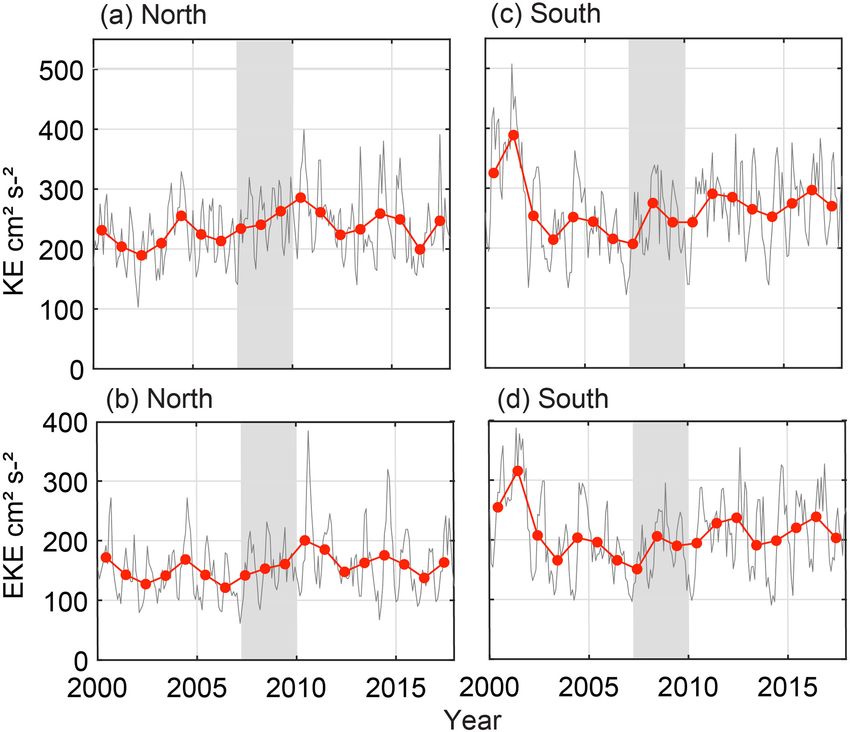
518 J. Kolbusz et al.: Mystery of the missing puerulus
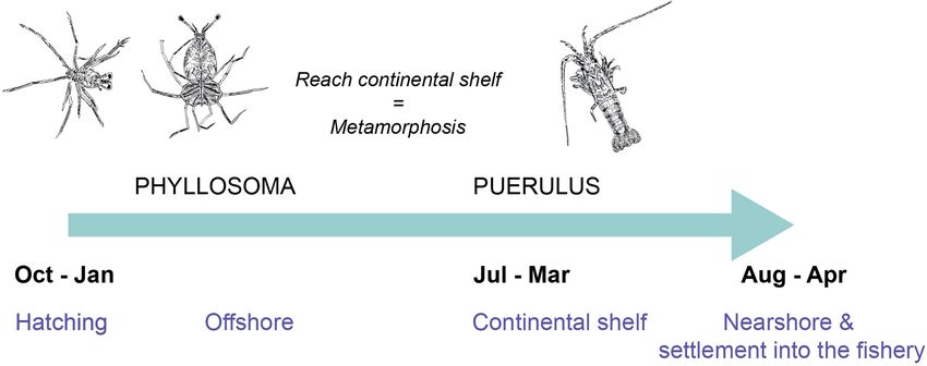
Figure 1. Early life cycle schematic of P. cygnus. Below the ar-
row indicates each stage’s approximate timing (black) and location
(blue). Above the arrow displays their growth, image credit Alice
Ford.
cline has been identified to date. Other research has shown
that, since the recovery in puerulus numbers, there has been
a latitudinal and timing shift in puerulus settlement compared
to historical data (Kolbusz et al., 2021). The majority of the
reduction has occurred in the first half of the puerulus set-
tlement season (May–October; Kolbusz et al., 2021). Addi-
tionally, in the southern sites, there has been a significant re-
duction over the whole season. In contrast, those in the north
have maintained levels of puerulus settlement during the sec-
ond half of the season (Kolbusz et al., 2021).
Between November and February, berried western rock
lobster females release their larvae (phyllosoma) throughout Figure 2. (a) Locations of puerulus survey sites included within this
the study region (Figs. 1, 2a). They are then transported off- study and other locations of note. The north and south refer to the
shore by the prevailing currents into the open ocean, where midpoint used in this analysis. The red boundary is the extent of en-
vironmental variables. The inset shows the location of the coastline
they transform through a series of temperature-dependent
in Australia. (b) Schematic of the major current systems thought
moults (Fig. 1). They undergo their final metamorphosis
to influence early-stage P. cygnus larvae movement. Relative arrow
into the actively swimming nektonic puerulus after approxi- size and location show characteristic currents. Eddies generated by
mately 8 months (Fig. 1). The onshore movement of pueru- the LC flow down the continental shelf are also indicated.
lus across the continental shelf peaks between September and
February (Phillips, 1981; de Lestang et al., 2018). Therefore,
circulation patterns of the southeast Indian Ocean influence
spatially varied cross-shelf transport of the puerulus (Caputi, (Pearce and Phillips, 1988; Lenanton et al., 1991). Conse-
2008; Feng et al., 2011). After a maximum of approximately quently, La Niña phases were also found to coincide with
30 d, they reach shallow areas of reef and seagrass habitats an above-average PI, thought to be due to a strengthened
as early juveniles (Feng et al., 2011). LC during these phases, with the Southern Oscillation Index
In the late 1960s, puerulus collectors resembling artificial (SOI) as an indicator of El Niño–Southern Oscillation phases
seaweed were developed and deployed at several shallow- (Clarke and Li, 2004; Caputi et al., 2001; Pearce and Phillips,
water sites within the fishery (Phillips, 1981). Puerulus are 1988). These relationships were identified through long-term
currently counted at eight sites spanning the latitude of correlations between the PI, FMSL, and SOI (Fig. 3). Since
the fishery, with the centrally located Dongara collectors 1988, studies have also demonstrated that the inter-annual
(Fig. 2a) now providing over 50 years of in situ data (Kol- variation in PI was influenced by the sea surface tempera-
busz et al., 2021). The puerulus settlement index (puerulus ture (SST) and westerly (onshore) winds (Caputi and Brown,
index, PI) is derived from these data, with the majority of 1993; Caputi, 2008; Caputi et al., 2010). Caputi et al. (2001)
puerulus settlement occurring between August and January defined a significant area overlapping with the spatial extent
(de Lestang et al., 2012). Therefore the puerulus settlement of the LC, where SST (27–34◦ S, 105–117◦ E) in February–
season occurs between May and April. April had a positive relationship with the PI of the subsequent
Research on the interaction between the physical environ- season. The bottom temperature during the spawning season
ment and PI began in the 1980s with a strong positive re- has also been identified as a cue for hatching and therefore
lationship found between the strength of the Leeuwin Cur- has a possible influence on the puerulus settlement season to
rent (LC), with Fremantle mean sea level (FMSL) as a proxy follow (Chittleborough, 1975; de Lestang et al., 2015).
Biogeosciences, 19, 517–539, 2022 https://doi.org/10.5194/bg-19-517-2022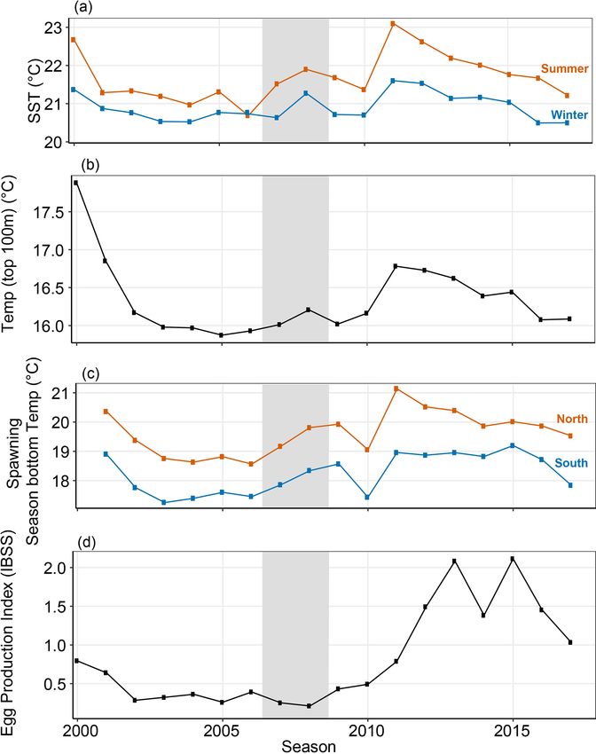
J. Kolbusz et al.: Mystery of the missing puerulus                                                                              519

   Following the decline in the PI in 2008 and 2009 (Fig. 3),       from the current’s forcing along the coastline may differ on
the aforementioned relationships between the PI and oceano-         either side of this latitude (Chittleborough, 1976; Berthot et
graphic factors broke down (de Lestang et al., 2015; Caputi         al., 2007). The El Niño–Southern Oscillation (ENSO) cy-
et al., 2014; Feng et al., 2011). Through one of the strongest      cle causes the pressure gradient to decrease (increase) dur-
La Niña phases on record (2011), the PI still did not recover       ing an El Niño (La Niña) episode, resulting in a weaker
to the previously expected high values (Boening et al., 2012;       (stronger) LC and cooler (warmer) sea surface temperature
Benthuysen et al., 2014). These changes have been gener-            SST (Pattiaratchi and Buchan, 1991; Feng et al., 2003; Wi-
ally attributed to increasing water temperatures during the         jeratne et al., 2018). This is supported by strong correlations
spawning period, resulting in an earlier onset of spawning,         between the Southern Oscillation Index (SOI as an indicator
and a decrease in the number of storms occurring near pueru-        of ENSO phases) and LC transport at 34◦ S with a 6-month
lus settlement (de Lestang et al., 2015). Since this decou-         lag (Schiller et al., 2008).
pling between proxy parameters and PI, additional years of             The LC is stronger during austral winter (May–July) and
contrasting settlement have been recorded, thus providing a         weaker during the austral summer (November–March) due
larger dataset to re-examine these relationships following the      to variations in the equatorial wind stress and the Aus-
period of low settlement.                                           tralasian monsoon season (January–March) (Pattiaratchi and
   This study aims to understand the recruitment failure and        Siji, 2020; Pattiaratchi and Woo, 2009; Smith et al., 1991;
subsequent shifts in settlement patterns, particularly regard-      Wijeratne et al., 2018). A weaker secondary peak in the LC
ing direct physical oceanographic parameters over the 9 to          also occurs over December–January (Wijeratne et al., 2018).
11 months before settlement. Previous research had high-            During the summer months, southerly wind stresses over-
lighted that the causal factor of the correlation between the       come the alongshore pressure gradient, moving upper layers
LC strength and PI before 2009 was unclear. Several sugges-         offshore and favouring upwelling onto the continental shelf
tions have been made as to whether it was due to the warmer         (Pearce and Pattiaratchi, 1999). The CC can be identified
waters the LC brings, high eddy retention of larvae close           through cooler waters initiated around 34◦ S with the cooler
to the coast, or better nutritional development within eddies       water extending to 27◦ S inshore of the LC (Fig. 2b) (Gers-
(Caputi et al., 2001; O’Rorke et al., 2015; Wang et al., 2015;      bach et al., 1999). The LC migrates offshore and is weaker
Lenanton et al., 1991). Other parameters defining the oceano-       over these sea-breeze-dominated summer months, whereas,
graphic conditions in the region, including the northward-          during winter, it floods the shelf and dominates the distribu-
flowing Capes Current (CC) (Fig. 2b), cross-shelf flows, and        tion of water masses (Cresswell et al., 1989; Pattiaratchi et
kinetic and eddy kinetic energy, have been previously sug-          al., 1997; Woo and Pattiaratchi, 2008).
gested as influencing the PI but not investigated (Hood et al.,        Mesoscale eddies have been identified in the LC system
2017; Koslow et al., 2008). The recent availability of high-        for more than 30 years (Andrews, 1977; Pearce and Grif-
resolution 3D numerical oceanographic model output over an          fiths, 1991; Cosoli et al., 2020). The LC, and its associated
extended period (Wijeratne et al., 2018) eliminates the need        flows, becomes unstable with the significant variations in to-
to use proxies to represent oceanographic processes. There-         pography over the latitudinal extent of the current, generat-
fore, we were able to calculate directly predicated oceano-         ing eddies, meanders, and offshoots (Batteen et al., 2007).
graphic parameters at various locations throughout the fish-        Therefore, as the LC strength increases, the system becomes
ery to investigate alongside puerulus settlement.                   more unstable, causing kinetic energy to increase (Feng et al.,
                                                                    2005; Pattiaratchi and Woo, 2009). The Abrolhos Islands at
                                                                    28.8◦ S and the narrowing of the continental shelf slope south
2   Study region                                                    of Dongara and the Perth Canyon are major topographic fea-
                                                                    tures for the preferential generation of these eddies (Fig. 2b)
Water circulation off the west coast of Australia is driven         (Feng et al., 2005; Meuleners et al., 2008; Rennie et al., 2007;
by the Leeuwin Current (LC) system that incorporates the            Huang and Feng, 2015; Cosoli et al., 2020). They have a
Leeuwin Current, the Leeuwin Undercurrent and summer                mean radius of ∼ 100 km and generally keep their original
wind-driven currents, and the Capes (CC) and Ningaloo               formation shape, lasting approximately 8 months (Fang and
(NC) currents, on the continental shelf (Fig. 2b) (Woo and          Morrow, 2003; Cosoli et al., 2020).
Pattiaratchi, 2008; Pattiaratchi and Woo, 2009). The LC is
generated through a meridional pressure gradient resulting
from the difference between lower-density water off north-          3     Methods
west Australia and the denser water of the Southern Ocean
(Hamon, 1965; Pattiaratchi and Buchan, 1991; Pearce and             3.1    Puerulus settlement data
Phillips, 1988). The mean southward volume transport of the
LC peaks around 32.8◦ S due to South Indian Counter Cur-            Puerulus settlement is surveyed year-round, currently at eight
rent input (Wijeratne et al., 2018). Near 28◦ S statistical anal-   sites across the fishery (between 34–27◦ S) using artificial
ysis has shown a break-point in the LC, suggesting responses        seagrass-like collectors (Fig. 2a). Sampling is conducted as

https://doi.org/10.5194/bg-19-517-2022                                                        Biogeosciences, 19, 517–539, 2022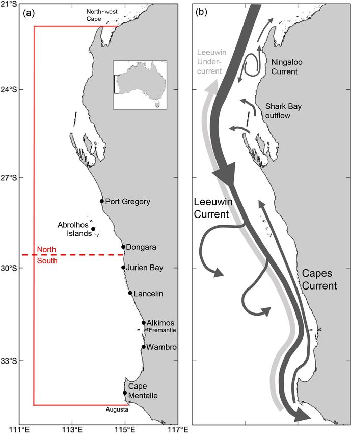
520                                                                             J. Kolbusz et al.: Mystery of the missing puerulus

Figure 3. Time series of annual (a) fishery-wide PI (May–April), (b) Fremantle mean sea level (FMSL) over June to December (m), and
(c) Southern Oscillation Index (SOI) (May–April). Grey shaded seasons indicate the less-than-expected PI based on a priori relationships
(Caputi et al., 2001). Blue and red shading indicate a La Niña and El Niño periods, respectively. Updated to 2018 and modified from Fig. 5
in Caputi et al. (2001).

close as possible to the full moon but may occur 5 d on ei-            cesses along the continental shelf, including tides, setting it
ther side of it. Therefore, puerulus are likely to have set-           apart from other ocean models for the same region. The grid
tled on the previous new moon period, giving approximately             was set at a horizontal spacing of 3 km to allow for topo-
monthly data (de Lestang et al., 2012). The monthly pueru-             graphic detail, providing predicted water movement. At the
lus settlement at each site is calculated as the average number        time of writing, ozROMS model output was available for
of puerulus per collector. For this study, we used the pueru-          the period 2000–2017. Details and validation of the model
lus settlement data from the 2001/02 season to 2016/17 at              are described by Wijeratne et al. (2018). Examination of this
each of the eight sites (Fig. 2), aligned with high-resolution         predicted dataset allows for the strength of the Leeuwin Cur-
oceanographic data hereafter detailed and estimates of west-           rent (LC), Capes Current (CC), and cross-shore transport to
ern rock lobster spawning biomass. Puerulus settlement data            be determined, as well as estimates of kinetic energy (KE)
for each site were split into “early” (May–October) and                and eddy kinetic energy (EKE) (Pattiaratchi and Siji, 2020).
“late” (November–April) portions, as described by Kolbusz              Their fluctuation is indicative of the conditions off the west
et al. (2021).                                                         coast of Australia.
                                                                          Monthly surface KE and EKE were calculated from
3.2     Oceanographic data                                             ozROMS to characterize the variability in the currents. A
                                                                       monthly time series was estimated following Eq. (1) for KE
To explore the variation in puerulus settlement, alongside the         and Eq. (2) for EKE:
prevailing oceanographic conditions, a single value for the                   s
respective early or late portion of the season was determined.                  u2 + v 2
Where relevant, the oceanographic variable was the same for            KE =              ,                                        (1)
                                                                                    2
both portions.                                                                 s
                                                                                  u0 2 + v 0 2
3.2.1    Numerical model outputs                                       EKE =                   ,                                  (2)
                                                                                       2
The Regional Ocean Modeling System (ROMS) has been                     where u and v are the monthly mean meridional and zonal
used in hindcast mode (past-time) for the whole of Australia           velocities, respectively (Caballero et al., 2008), and u and
(ozROMS) to resolve subsurface and surface currents and the            v are the monthly averages with the climatological means
associated volume transports (Wijeratne et al., 2018). This is         subtracted to remove seasonality (Luo et al., 2011). The
a fully three-dimensional circulation model, resolving pro-            months that phyllosoma are offshore, depending on when

Biogeosciences, 19, 517–539, 2022                                                           https://doi.org/10.5194/bg-19-517-2022
J. Kolbusz et al.: Mystery of the missing puerulus                                                                             521

they have hatched, can be between October (year − 1) and            of the whole spawning season (September–March). Due to
March (year + 1) (Fig. 2). Therefore, the calendar year from        the ozROMS hindcast starting in 2000, values were only
January to December was used to obtain an average for the           available from the 2001 season since the spawning season
offshore conditions spanning the possible time frame off-           is the calendar year prior to settlement. Despite de Lestang
shore. Due to different mean oceanographic conditions, we           et al. (2015) using monthly values, we found only a small
considered a north and south offshore box (Fig. 2a) that cov-       amount of variation between the months and therefore used
ered the approximate extent of where phyllosoma are trans-          a single bottom temperature value to represent a season. The
ported (Feng et al., 2010, 2011; Berthot et al., 2007). For our     temperature in the top 100 m of the water column, east of
analysis, we have not defined the directionality and size of        108◦ E, as a mean annual value from ozROMS was also in-
eddies. Still, it is an important consideration pertinent to lar-   cluded. This accounts for temperature variation over the mi-
vae energy stores that would require further modelling out-         grating depths phyllosoma occupy over their early pelagic
side the scope of the current study (Cetina-Heredia et al.,         life cycle (Griffin et al. 2001; Feng et al. 2011).
2019b).
   The monthly transport estimates of LC and CC (in sver-           3.2.2    Satellite-derived sea surface temperature (SST)
drups, Sv = 106 m3 s−1 ) were derived using the ozROMS
hindcast dataset (Wijeratne et al., 2018). The transport for        Satellite-derived SST data for the study region were obtained
each current was defined as follows: (1) CC as northward            from the Integrated Marine Observing System (IMOS) Aus-
volume transport of water across latitudes 27, 30, and 34◦ S        tralian Ocean Data Network (AODN) portal (https://portal.
in water depths less than 100 m and (2) LC as southward vol-        aodn.org.au/, last access: 1 March 2021). The climatology
ume transport of water across latitudes 27, 30, and 34◦ S but       data, centred on the base period 1993–2020, SST Atlas of
in water depths greater than 100 m but limited to the upper         Australian Regional Seas (SSTAARS) (Wijffels et al., 2018),
300 m of the water column (Table A1, Appendix A). For the           were used to derive monthly SST anomalies for the region
LC austral winter strength, the transport over June, July, and      extending offshore to 108◦ E (extent in Fig. 2; see also Pat-
August was averaged, and for summer December, January,              tiaratchi and Hetzel, 2020). This was to reflect the exten-
and February were averaged. The LC summer period corre-             sive duration (∼ 9 months) of the pelagic larval and pre-
sponds to recently hatched larvae (spawning season, s − 1),         settlement stage of P. cygnus (Phillips, 1981). All monthly
leaving the continental shelf and puerulus returning in the         SST anomalies were initially included in the analysis due
late portion of the season (settlement season, s) (Fig. 2). The     to the likely importance of temperature on all stages of the
LC winter period corresponds to when puerulus are return-           pelagic larval stage (Caputi et al., 2001; de Lestang et al.,
ing to the shelf (settlement season, s). The CC strength was        2015).
divided into early (September, October, and November) and
                                                                    3.3     Independent breeding stock survey (IBSS)
late (December, January, February, and March) and corre-
sponded to the time when recently hatched larvae were leav-         Independent breeding stock surveys (IBSSs) have been con-
ing the continental shelf (spawning season, s − 1) and pueru-       ducted annually since 1992 over the last new moon (∼ 15
lus were returning in the early and late portions of the settle-    November) before the start of the fishing season (de Lestang
ment season respectively (Fig. 2).                                  et al., 2018). The catch rates of spawning females from this
   Cross-shelf transport (in sverdrups) was calculated for          survey (adjusted for fecundity) provide a standardized egg
each monthly time step between the depth contours (200–             production index. It is conducted at up to six sites spanning
50 m) over 2◦ latitudinal bins (26–28, 28–30, 30–32, and 32–        the fishery and close to the peak in egg production (Novem-
34◦ S) (Table A1, Appendix 1). These latitudinal bins were          ber) (Caputi et al., 1995; Chubb, 1991; de Lestang et al.,
chosen closest to account for differences in topography and         2016). Therefore, IBSS was included in our analysis, ac-
cross-shelf flow differences across the survey sites. Monthly       counting for variability in the number of hatching larvae.
averages for each latitudinal bin indicated that the variability
in transport is highest over April to September. These months       3.4     Generalized additive modelling
correspond to the eastward “on” movement of puerulus. Re-
cently hatched larvae cross the shelf (westward, “off” in the       The oceanographic variables likely to influence water move-
spawning season) to the open ocean between September and            ment and the distribution and survivorship of P. cygnus, de-
March (Fig. 2). These two sets of months were averaged to           tailed above, were considered predictors of the puerulus set-
get values of cross-shelf transport (as phyllosoma “off” and        tlement within a generalized additive model (GAM). In ad-
as larvae “on”) for each season (Fig. 2).                           dition, the IBSS was included as a predictor to include vari-
   Temperatures in the model layer immediately above the            ability in the number of hatching larvae. Due to the extensive
seabed (“bottom temperature”) over the spawning depths              latitudinal range of the settlement data, some environmental
(40–80 m) were retrieved from ozROMS due to the absence             variables were dividing into northern, central, or southern ar-
of in situ data (de Lestang et al., 2015). The predicted values     eas depending on the data type and availability. A value was
were averaged over a northern and southern subset (Fig. 2a)         obtained for each possible predictor variable to align with

https://doi.org/10.5194/bg-19-517-2022                                                       Biogeosciences, 19, 517–539, 2022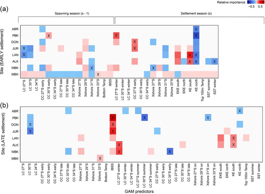
522                                                                         J. Kolbusz et al.: Mystery of the missing puerulus

each half of the puerulus season (Appendix A, Table A1).           dictors of the early puerulus settlement at sites (eight) (Ap-
Firstly, linear regression analysis was performed to assess        pendix A, Table A1). LC strength in summer and the late CC
whether strong (> 0.70) correlations existed between vari-         strength predictors for early settlement were omitted since
ables. Where valid, a case-by-case approach was taken to de-       they occur after early settlement each season. Given the pre-
termine whether both, an average, or one of the two variables      dicted data availability and the spawning season being in the
was included in the overall model before the time series mod-      calendar year prior, the relationship between all predictors
elling – this eliminated potential problems with collinearity      and puerulus settlement was limited to the 2001 to 2017 sea-
and overfitting (Graham, 2009). Bottom temperatures were           sons.
all highly correlated (> 0.89) and therefore averaged to give         The R language for statistical computing (R Core Team
a single variable. Co-correlation between the SST of adjacent      2018) was used for all data manipulation (dplyr; Wickham et
months led to a winter and summer average being used.              al. 2018) and analysis (Wood, 2017) (mgcv; Wood, 2011). In
   GAMs with full subset model selection (FSSgam) were             addition, MATLAB and the M_map toolbox were used for
used to investigate the influence of the final 16 (8, early and    any spatial plotting (MATLAB, 2019b; M_Map: A mapping
late settlement periods) different response variables (Fisher      package for MATLAB, Version 1.4 m).
et al., 2018). Predictors were initially limited to a maxi-
mum of three knots per spline. However, due to the relatively      3.5    Exploration of variation in oceanographic
small sample size and heterogeneous distribution of the pre-              conditions
dictors, cross-shelf transport remained, but other predictors
were treated as linear relationships. Model sizes were lim-        Seasonal and inter-annual variability, not captured within the
ited to three predictors to prevent overfitting. Model selection   GAM, was explored graphically with the inclusion of mov-
was based on Akaike’s information criterion (AIC; Akaike,          ing means. An extended period of low activity was expe-
1973) optimized for small sample sizes (AICc; Hurvich and          rienced in the southeast Indian Ocean between 2001 and
Tsai, 1989). The best models selected were the most parsi-         2007 (Pattiaratchi and Siji, 2020). Given that processes in the
monious within two AICc units of the model with the lowest         ocean do not respond instantaneously, these “hiatus” condi-
AICc (Burnham and Anderson, 2002). Importance scores for           tions were explored as a whole. ENSO information (SOI) and
each variable were obtained by summing the AICc weights            the Fremantle mean sea level (FMSL) were obtained from
of each model that each variable occurred within (Fisher et        the Bureau of Meteorology (2022a, b). Altimeter data were
al., 2018).                                                        accessed from the IMOS AODN to investigate the relation-
   Table 1 shows each predictor variable and the associated        ship between the PI and the energy system, in particular, the
hypotheses for each annual value. The LC consistently flows        long-term KE and EKE over the southeast Indian Ocean (Pat-
southwards and is strongest over the winter months, possi-         tiaratchi and Siji, 2020)
bly flooding the shelf. Therefore, over the winter months,            During the summer, the interactions between the Capes
this would likely positively affect late-stage phyllosoma suc-     Current and Leeuwin Current were also addressed (Pat-
cessfully reaching the nearshore. Over the summer months,          tiaratchi and Woo, 2009). First, the LC and CC summer pe-
the LC strength, if stronger, would likely impede the sur-         riod strengths were standardized for each season, and then
vival of early-stage phyllosoma (Feng et al., 2011). Given the     the difference between the two was plotted alongside the
stronger opposing LC, the northward-flowing CC on the shelf        early and late puerulus settlement levels.
would likely positively impact puerulus settlement (Muh-
ling et al., 2008). Kinetic energy will likely positively im-
pact the transportation of phyllosoma throughout their early       4     Results and discussion
pelagic life cycle (Cetina-Heredia et al., 2019a; Hood et al.,
2017). Similarly, cross-shelf transport offshore would likely      Our findings demonstrate that similar oceanographic con-
increase the survival of phyllosoma, and cross-shelf transport     ditions influence adjacent puerulus monitoring sites. The
onshore after the pelagic phase would assist puerulus trans-       Leeuwin Current strength over the summer months has in-
portation onshore. P. cygnus spawning likely occurs sooner         creased since the low puerulus settlement season, alongside
with an increased bottom water temperature, causing pos-           a decrease in the Capes Current, suggesting a mismatch in
sible timing mismatches over the next 9 to 11 months (de           the puerulus transport processes. In addition, this period oc-
Lestang et al., 2015). Conversely, warmer water temperatures       curred alongside neutral ENSO conditions and cooler wa-
increase the rate of phyllosoma development, therefore likely      ter over the likely P. cygnus pelagic distribution. These re-
increasing their survival (Phillips et al., 1978; de Lestang et    sults and their discussion are in the following three sections:
al., 2015). If the IBSSs were higher, there would be more          (1) time series exploration of P. cygnus settlement between
spawning stock and therefore likely an increase in phyllo-         2001 and 2017 and associated oceanographic conditions ex-
soma and eventual puerulus (de Lestang et al., 2012). These        perienced by the larvae to represent each puerulus settle-
variables resulted in a total of 39 possible predictors of the     ment season (May to April), (2) exploring the correlation
late puerulus settlement (eight sites) and 33 possible pre-        of oceanographic conditions with settlement data through a

Biogeosciences, 19, 517–539, 2022                                                      https://doi.org/10.5194/bg-19-517-2022
J. Kolbusz et al.: Mystery of the missing puerulus 523
Table 1. Predictor variables and metrics used in the GAM analysis to investigate variability in puerulus settlement and associated hypothesis.
The subscript s identifies the relativity of a month to the puerulus settlement season (May–April) in question. s − 1 is within the season prior
and s + 1 is after. − denotes a negative relationship, and + denotes a positive relationship.
Predictor variable Metric used Hypothesized relationship to puerulus
settlement
Leeuwin Current (LC) Southward strength of the current in sverdrups (Sv) at (1) − (all sites)
northern, central, and southern locations for three periods: (2) + (all sites)
(1) larvae hatching/transport offshore (Decs−1 –Febs−1 ) (3) − (north sites), + (south sites)
(2) puerulus transport towards continental shelf (Mays –
Junes )
(3) peak settlement (Decs –Febs )
Capes Current (CC) Northward strength of the current in Sv at a north, two (1) + (all sites)
central, and a south location over two periods: (2) + (north sites), − (south sites)
(1) larvae hatching/transport offshore (Seps−1 –Novs−1
(early) and Decs−1 –Febs−1 (late))
(2) peak settlement (Seps –Novs (early) and Decs –
Febs (late))
Kinetic and eddy kinetic Kinetic and eddy kinetic energy of the southeast Indian (1) + (all sites)
energy Ocean in cm2 s−2 over a north and south area defined in
Fig. 2a:
(1) phyllosoma offshore
(Jans−1 –Decs )
Cross-shelf transport Cross-shelf transport over the continental shelf (150–50 m) (1) Westerly (−0 Sv) +
in sverdrups over a northern and two central and southern (2) Westerly (+Sv) −0
latitudinal bins:
(1) larvae hatching/phyllosoma transport west (Seps−1 –
Mars−1 )
(2) puerulus transport east (Aprs−1 –Seps )
Temperature Water temperature over three periods: (1) SST + (all sites)
(1) SST summer (Seps−1 –Mars−1 ) and SST winter (2) − (all sites)
(Aprs−1 –Augs ) (3) + (all sites)
(2) bottom temperature during spawning (40–60 m depth,
Seps−1 –Mars−1 )
(3) top 100 m
early-stage phyllosoma
(Jans−1 –Decs )
Independent breeding stock (1) IBSS index for the spawning season (1) + (all sites)
surveys (IBSSs)
general additive model analysis, and (3) inter-annual and sea- The three temperature variables (SST, top 100 m temper-
sonal oceanographic variability. ature and bottom temperature) all followed a similar pattern
to one another (Fig. 5a–c). They gradually decreased from
highs in 2000 to a low in 2005 before slightly increasing from
4.1 Time series patterns
2008, all reaching maxima in 2011 when a marine heatwave
occurred in February (Wernberg et al., 2012). A decrease
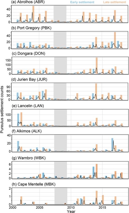
Puerulus settlement differs dramatically over the latitudes of of approximately 1–2 ◦ C in bottom temperature during the
the fishery, with central latitudes experiencing the highest spawning season was evident over the early 2000s, which
numbers (Fig. 4). At the Abrolhos (Fig. 4a), the late settle- shifted over the low-PI seasons (grey seasons, Fig. 5a–c). It
ment is consistently higher and remained consistent after the then increased again by 2012 (Fig. 5). Until the heatwave,
recruitment failure, which is expected (Kolbusz et al., 2021). the variation in PI at some sites (Lancelin and Port Gregory)
Other sites display similar early and late puerulus settlements additionally aligned with the SST fluctuations. This is likely
before 2008. However, after 2009, recovery occurs predomi- the bottom temperature variation captured by de Lestang et
nately in the latter half (Fig. 4a, c, d, and e).
https://doi.org/10.5194/bg-19-517-2022 Biogeosciences, 19, 517–539, 2022
524                                                                          J. Kolbusz et al.: Mystery of the missing puerulus

                                                                     Figure 5. Parameters calculated for seasonal analysis of PI. (a) Sea
                                                                     surface temperature (◦ C) from 24–34◦ S and out to 108◦ E obtained
                                                                     from the SSTAARS daily dataset on the IMOS AODN portal from
                                                                     1996 to 2016. (b) Temperature in the top 100 m of the offshore area
                                                                     from 24–34◦ S and east of 108◦ E over January–December, the av-
                                                                     erage time phyllosoma are offshore. (c) Average bottom tempera-
                                                                     ture (40–80 m depths) (◦ C) of the spawning season for associated
                                                                     PI season for October to March in the northern (blue line, shown in
Figure 4. Monthly average puerulus counts for each monitor-          Fig. 2a) and southern latitudes (red line, shown in Fig. 2a) of the
ing site (black line) with the early (May–October, blue) and late    fishery. (d) The independent breeding stock survey index (IBSS)
(November–April, red) puerulus settlement for the season. The in-    lagged 1 year to give a spawning stock index for the year prior (de
dex is a sum of the included monthly average puerulus counts. Grey   Lestang et al., 2016). Grey shaded seasons (2008 and 2009) indicate
shaded seasons (2008 and 2009) indicate the less-than-expected PI    the less-than-expected PI based on a priori relationships (Caputi et
based on a priori relationships (Caputi et al., 2001).               al., 2001).

al. (2015). The winter months (June to August) had less than         2008 and 2009, restrictions to fishing were designed to pre-
1◦ of between-year annual variability over the entire tempo-         serve spawning biomass. Therefore the IBSS was expected
ral scale.                                                           to increase.
   The IBSS was consistently under 0.5 from 2002 until the              The LC was the strongest over the winter months, reaching
2011 season before increasing 3-fold by 2013 to record highs         7 Sv in the 2000 season at 34◦ S (Fig. 6a). However, the sum-
(Fig. 5) (de Lestang et al., 2016). Previous studies have not        mer LC was strongest in 2010, at 27◦ S. Both values align
found the IBSS to be implicated in the recruitment failure           with strong La Niña conditions (Boening et al., 2012). This
(de Lestang et al., 2015). However, it was included in the           maximum, however, did not correspond to a maximum in
current analysis for completeness and because studies of             winter LC strength (Fig. 6b) (Wijeratne et al., 2018). Over
recruitment failures in other fisheries have frequently sug-         the initial months of the CC forming (Fig. 6c), it is, on aver-
gested spawning biomass to be a factor (Guan et al., 2019;           age, strongest at 30◦ S. The CC displayed a roughly similar
Ehrhardt and Fitchett, 2010). In addition, the IBSS increased        pattern across all latitudes with less variability in current at
from 2011; this is likely due to the restrictive fishery manage-     27◦ S where it is weakest (Fig. 6c and d). CC minima occur
ment. After the lower-than-expected puerulus settlement in           over the 2010 to 2012 seasons in the early and late strength

Biogeosciences, 19, 517–539, 2022                                                         https://doi.org/10.5194/bg-19-517-2022
J. Kolbusz et al.: Mystery of the missing puerulus                                                                                    525

Figure 6. Leeuwin (LC) and Capes (CC) current strengths at 27, 30, and 34◦ S. (a) LC (southward transport, Sv) over winter (May–July)
and (b) summer (December–February). (c) CC (northward transport, Sv) (c) over the early portion of the summer (September–October) and
(b) late portion of the summer (December–March). Grey shaded seasons (2008 and 2009) indicate the less-than-expected PI based on a priori
relationships (Caputi et al., 2001).

signals (Fig. 6c and d). Spatial variations in the LC and CC
were distinguishable with increased LC at the southern lati-
tude (Fig. 6a and b) and the strongest CC signature at 30◦ S
(Fig. 6d) as reported previously by Wijeratne et al. (2018).
   Water circulation at all latitudes of the fishery was predom-
inantly driven by the LC, with the changing topography down
the coast causing less onshore flow on average within the
centre of the fishery (29◦ S) (Rennie et al., 2007; Feng et al.,
2010; Wijeratne et al., 2018). Regions with a wider continen-
tal shelf generally have higher retention of waters, therefore
causing less cross-shelf transport of water. Depth-averaged
cross-shelf transport of water was predominantly onshore at
both 33 and 29◦ S (Fig. 7). This was not unexpected given
the steep topography of the continental shelf and LC inter-
actions. Average monthly variations in cross-shelf transport
indicated that between April and September onshore trans-
port increased at 33 and 29◦ S; however, it decreased at 31
and 27◦ S (Fig. 7). Coastal geographic features increase the
spatial heterogeneity over the latitudes and how the LC in-
teracts with the nearshore (Feng et al., 2010). At 27◦ S, on
average offshore transport was possibly due to more mixing
and a wider continental shelf. This is due to the topography
of Shark Bay and the contribution of the Ningaloo Current
                                                                       Figure 7. Cross-shelf transport (easterly) between 200–50 m over
(Fig. 2b), likely playing a role (Woo and Pattiaratchi, 2008).
                                                                       2◦ latitudinal bins (26–28, 28–30, 30–32, and 32–34◦ S). Averaged
   Variations in EKE and KE over the time series show ap-
                                                                       for the (a) spawning “off” transport season (September–February,
proximately 5-yearly patterns (Fig. 8) in fluctuation with             season −1) and (b) settlement “on” transport season when varia-
maxima in 2000, 2005, and 2011 aligning with ENSO events               tion in cross-shelf transport is the highest (April–September). Grey
(Pattiaratchi and Sijim 2020). From 2002 to 2008, the KE               shaded seasons (2008 and 2009) indicate the less-than-expected PI
and EKE were relatively low, indicating a weaker LC over               based on a priori relationships (Caputi et al., 2001).
those seasons. Particularly over the southern box, the de-
crease in KE and EKE and recovery by 2012 show similar

https://doi.org/10.5194/bg-19-517-2022                                                            Biogeosciences, 19, 517–539, 2022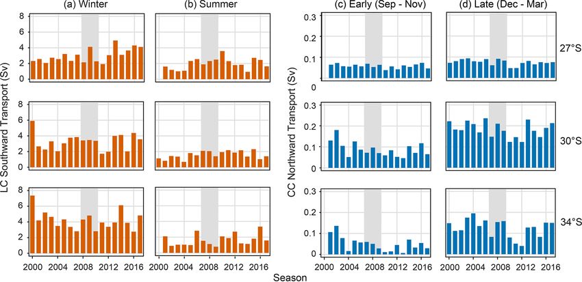
526                                                                             J. Kolbusz et al.: Mystery of the missing puerulus

                                                                        pears spurious. However, the southern and central flows of
                                                                        the South Indian Countercurrent (sSICC, cSICC) flow east-
                                                                        ward within the southern and northern KE “boxes” respec-
                                                                        tively (Menezes et al., 2014). These current jets connect with
                                                                        the LC and may cause the temporal and spatial difference in
                                                                        KE and subsequent influences on puerulus settlement. In par-
                                                                        ticular, for the Abrolhos, KE in the north is within the most
                                                                        parsimonious model for early and late settlement. Due to the
                                                                        sites’ location offshore, increased water movement may pre-
                                                                        vent puerulus from successfully settling on the islands within
                                                                        the defined area of KE. Instead, they could swim elsewhere
                                                                        with less resistance. This difference in KE relationships sug-
                                                                        gests different driving mechanisms over the fishery on both
                                                                        the temporal (early and late) and spatial (north and south)
                                                                        scales.
                                                                           The model results provide clues regarding the influence of
Figure 8. Monthly kinetic energy and eddy kinetic energy (grey)         the LC and CC (LC winter, LC summer, CC early and late)
with yearly averages (January–December) (red). North and south          on phyllosoma when they are in later life stages. Interest-
divides are shown in Fig. 2a. (a) KE (cm2 s−2 ) in the north. (b) EKE   ingly, the LC during the spawning season at 27◦ S was within
(cm2 s−2 ) in the north. (c) KE (cm2 s−2 ) in the south. (d) EKE        the most parsimonious model for Lancelin early settlement as
(cm2 s2 ) in the south. Grey shaded years (2008 and 2009) indicate      a negative relationship (Fig. 9a). Thus, for Lancelin, the LC
the less-than-expected PI based on a priori relationships (Caputi et    may have been too strong for some early-stage phyllosoma
al., 2001).                                                             to cross the shelf, to get westward, without being swept too
                                                                        far south for survival. Especially given the steep continental
                                                                        shelf at this latitude. In winter, a stronger LC (puerulus reach-
patterns to the puerulus settlement (grey years, Fig. 8c and            ing the continental shelf) and a stronger CC (puerulus settling
d). Additionally, the southern box shows increased variabil-            on reefs) were suitable for early settlement at Dongara. This
ity, suggesting greater variability in the LC at southern lati-         was a hypothesized result (Table 1) and was also consistent at
tudes (Fig. 8c and d). Conversely, the northern values, par-            adjoining sites (Port Gregory for LC and Jurien Bay for CC,
ticularly for KE, increased over the same time frame, with              Fig. 9a) (Pearce and Pattiaratchi, 1999). For later settlement,
less variability (EKE), indicating that different forcing mech-         the opposite relationships occur. The LC in summer has a
anisms, such as the South Indian Countercurrent, may play a             negative relationship to Port Gregory (and Abrolhos), and
role (Fig. 8c and d).                                                   the CC has a negative relationship with Warnbro (Fig. 9b).
                                                                        This was expected for Port Gregory, a northern site, to be
4.2   Generalized additive model                                        negatively influenced by the southward-flowing current (LC),
                                                                        transporting puerulus further southward. Similarly, southern
The generalized additive model (GAM) analysis shows that                sites are negatively influenced by the northward-flowing cur-
puerulus settlements at adjacent sites tend to be influenced            rent (CC), transporting puerulus northward. However, these
by similar oceanographic variables. However, the Abrolhos               trends become vague over the central latitudes of the fishery
(northernmost and offshore) and Cape Mentelle (southern-                where little to no relationship is found, especially during the
most) sites are unique (Fig. 9, Appendix B). The most signif-           summer of hatching (Fig. 9a, CC 27◦ S early). This draws at-
icant relationships did vary between the early and late por-            tention to the spatial and oceanographic heterogeneity of the
tions of the seasons and between sites, as expected (Table 1).          study sites. Given the mix of expected and unexpected and
Those of note are discussed hereafter.                                  strong and weak results from the multiple regression analy-
   In contrast to our predictions (Table 1), sites were corre-          sis, particularly for the early settlement, it is clear complex
lated by a negative relationship to KE in the north for early           forcing’s are at play in the system, with both currents flowing
settlement (Fig. 9a). This correlation was more robust for the          in opposing directions perpendicular to the direction pueru-
northern sites. A strong KE implies a strong LC signature               lus are swimming. The influence of factors found to have the
over the defined spatial area (Fig. 2a). Comparatively, EKE             strongest correlation on puerulus settlement is presented in
and KE in the south had positive relationships to sites in the          the following Sect. 4.3.
centre of the fishery for early and late settlement, suggesting            The IBSS shows a strong positive relationship with Port
a different forcing could be at play (Fig. 9). This was alluded         Gregory, Dongara, Jurien Bay, Lancelin, and Warnbro over
to within the time series analysis (Fig. 8). The possibility that       the late settlement. However, it has little relationship with the
two adjacent parts of the southeast Indian Ocean would have             early settlement (Fig. 9a and b). Nevertheless, these positive
opposing effects on the settlement at only two locations ap-            relationships corroborate that the egg production influences

Biogeosciences, 19, 517–539, 2022                                                           https://doi.org/10.5194/bg-19-517-2022
J. Kolbusz et al.: Mystery of the missing puerulus 527
Figure 9. Variable importance scores within 2 AIC of the top model from the multiple linear regression analysis (GAM) to predict the
(a) early and (b) late settlement at sites. Full results are in Appendix Tables B1 (early) and B2 (late). The timeline (above) indicates the
timing of the variables from either the spawning season (s − 1) where larvae are moving offshore (westward) or the settlement season (s)
where larvae are moving eastward. Positive (red), zero (white), and negative (blue) relationships with variables are shown, and variables
within the most parsimonious model for each site are indicated (X).
the number of larvae returning to the coast as puerulus and
may more accurately represent the spawning stock of pueru-
lus reaching the coast over the latter half of the settlement
season. Given the longer time series available for the IBSS
and Dongara settlement, we reanalysed the relationship for a
more extended period. We found that pre-2000 IBSS is a rea-
sonable predictor with an R 2 of 0.434 and explaining 30.3 %
of the deviance in the Dongara settlement (Fig. 10). In an
ideal scenario, one would expect all sites, both early and late,
to have a relationship with the spawning stock. For locations
where increased IBSS did not positively correlate with PI, it Figure 10. Observed (black) and modelled (red) late Dongara
may be solely that the influence of oceanographic factors on (DON) settlement index from 1993 to 2018. The red line is the most
the puerulus settlement was more substantial. parsimonious model extended to 1993.
Cross-shelf transport shows irregular patterns between the
sites. Cross-shelf transport for the spawning season (27, 29,
and 33◦ S, Fig. 9a) has some positive links to increased set-
at different locations. Average cross-shelf transport has pre-
tlement in the early half of the season for sites south of Don-
viously indicated a break over the mid-latitudes of WA (Wi-
gara. However, this is the opposite for 31◦ S (Fig. 9a), but
jeratne et al., 2018, Fig. 9).
these relationships are less pronounced over settlement later
On an annual timescale, increased strength in KE in the
in the year (Fig. 9b). Various transportation pathways are
northern offshore areas of the fishery (Fig. 1) was associ-
likely working in opposing directions to influence settlement
ated with a decrease in puerulus settlement in the early por-
https://doi.org/10.5194/bg-19-517-2022 Biogeosciences, 19, 517–539, 2022528 J. Kolbusz et al.: Mystery of the missing puerulus
tion of the season. It is not uncommon for the advective be- ious oceanographic mechanisms act differently, sometimes
haviour of large-scale eddies to negatively affect crustacean in competition (Fig. 9a, b), to provide contrasting results
species (Medel et al., 2018; Nieto et al., 2014). Retention for the different sites. Using the above multiple regression
and dispersal of larvae can also differ in persistent eddy sce- analysis results as an exploratory tool, we have additionally
narios where a more uniform shape likely leads to retention. drawn upon patterns in the southeast Indian Ocean and WA
However, a more eccentric shape leads to dispersal (Cetina- coastal zone over the last 2 decades. This includes lagging
Heredia et al., 2019b). Earlier studies suggest an increase in conditions, alongside the fishery changes, that may have con-
the number of eddies positively influences the retention of tributed to the “worst-case scenario” and resulted in the re-
larvae and, therefore, transport across the shelf and to the cruitment failure in 2008–2009.
nearshore (Griffin et al., 2001; Yeung et al., 2001; Cetina-
Heredia et al., 2019a, 2015). This is contradictory to our re- 4.3.1 Inter-annual: hiatus period and cross-shelf
sults. Our study used the mean annual KE over a large spatial transport
area, and the site in question is north of the highest density of
puerulus settlement. Using a large spatial area, we have omit- Over the past 30 years, links between ENSO events and the
ted the influence of sub-mesoscale features within the region, PI have been well documented using the SOI (Fig. 3) (Caputi
which could impact a puerulus’ ability to cross the shelf and et al., 2001; Pearce and Phillips, 1988). Warmer temperatures
reach coastal habitats (Cosoli et al., 2020). are experienced during stronger LC conditions evident dur-
The GAM analyses suggest that different environmental ing the La Niña phase (positive SOI), providing better condi-
drivers influence PI at each site, but this varies depending tions for larval development. The SOI record since these re-
on when puerulus return to shore (early or late, Fig. 9a, b). lationships began highlights the possibility of sustained neu-
However, we can establish discernible patterns with some tral ENSO conditions being a reason for this breakdown (Pat-
certainty and physical relevance. Sites closer in latitude have tiaratchi and Hetzel, 2020; Pattiaratchi and Siji, 2020). From
similar results, Abrolhos and Cape Mentelle being the excep- 2000 until 2009, neither a moderate La Niña phase nor a
tions. Abrolhos is located off the shelf and has historically moderate El Niño phase occurred, and consequently, the en-
had different trends in PI compared to other locations and ergy in the system also decreased (Fig. 3). After 2009, an
even on the adjacent coast. The Abrolhos PI has also recov- unusually strong LC (La Niña, 2011) was preceded by an un-
ered to pre-failure levels, whereas coastal locations have not, usually weak year (El Niño, 2010) (Huang and Feng, 2015).
particularly at Lancelin and locations further south (Kolbusz Before 2008 there were fluctuations in LC strength, or phases
et al., 2021). Cape Mentelle has historically had a low settle- of moderate strength, over several seasons whilst the pueru-
ment and also has a unique location being the farthest south. lus settlement also fluctuated similarly (Fig. 3, Caputi et al.,
Early settlement at Cape Mentelle also showed little differ- 2001, Fig. 6). An extended period (> 5 years) of low or neu-
ence between all top models within 2 AIC of the most parsi- tral ENSO conditions, termed a hiatus, had not yet been ex-
monious model (cross-shelf transport at 33◦ S during spawn- perienced since puerulus collection began; therefore, the re-
ing season). Despite one variable having the highest impor- lationship breakdown is not surprising. Recovery in puerulus
tance and being in the top model, there was little difference numbers began after the strong La Niña in 2011, taking a
between all models within 2 AICc units. few seasons to reach levels before 2000. If these strong La
Given the several months over which lobster larvae hatch, Niña conditions had not occurred, what would have been the
followed by their prolonged pelagic life cycle and settlement response? Whether this delayed recovery was due to the cli-
estimated to occur some 9–11 months later (Phillips, 1981), mate inertia in the system adjusting or changes in recruitment
the large amount of variation and lack of solid relationships numbers after changes in the fishing the spawning stock is
between environmental or biological predictors and PI was uncertain.
not unexpected (Fig. 2). However, we have revealed patterns Similarly, SST anomalies (Fig. 11) have periods of neu-
up and down the coast, suggesting that both biological and tral conditions and below-average temperatures, respectively,
environmental predictors can have a strong and sometimes from approximately 2000 to 2008 (Pattiaratchi and Het-
consistent influence on puerulus settlement for adjacent sites. zel, 2020). These extended low-activity conditions may have
caused a shift in the conditions experienced by pelagic west-
4.3 Variation in oceanographic conditions ern rock lobster larvae. The patterns may be due to atmo-
spheric and oceanic processes that imprint themselves upon
All the oceanographic factors examined here have been sug- the SST field. The ocean’s thermal energy is transferred to
gested to directly influence P. cygnus larvae at some point the atmosphere via the sea surface, which the SST controls.
in their first year of life. Over time, the forcing and interac- Thus, SST on a spatial scale plays a crucial role in regulat-
tions between these environmental variables were too com- ing climate and variability. The extended period of cooler
plex to examine in the multiple regression analysis. However, SST anomalies may have contributed to the low 2008 and
they may have as much influence on successful puerulus set- 2009 settlements. A decreasing PI over the start of the cen-
tlement as instantaneous values used. Furthermore, the var- tury was in line with these patterns. Then recovery followed
Biogeosciences, 19, 517–539, 2022 https://doi.org/10.5194/bg-19-517-2022J. Kolbusz et al.: Mystery of the missing puerulus 529
Figure 12. Cross-shelf transport (easterly) between 2000 and 2018
off the shelf. North and south divides are shown in Fig. 1a. North
cross-shelf flux between (a) 250–150 m and (b) 75–25 m. South
Figure 11. (a) Kinetic energy and (b) eddy kinetic energy cross-shelf flux between (c) 250–150 m and (d) 75–25 m. The
(cm2 s−2 ) from altimeter data, the (c) SST (◦ C) anomaly from yearly moving mean (red) and the positive and negative moving
SSTAARS, and (d) PI for the whole western rock lobster fishery. standard deviations (dashed black) are included.
the maxima experiences with the 2011/12 La Niña (Boening
et al., 2012), which perhaps took the system some years to
return to conditions as usual. Thus, it may not be a season-
specific factor that caused the years of low settlement in the
late 2000s. Instead, consecutive years of these hiatus con-
ditions (Fig. 11) have driven a regime shift in the environ-
ment, impacting P. cygnus pelagic life stages (DeYoung et
al., 2004).
Despite cross-shelf transport being a forcing mechanism
behind larval transport into the nearshore, a lack of statisti-
cal relationships was found through the multiple regression
analysis. Given the hiatus conditions or shift after 2008 in the
LC, one would expect some form of accompanying change
in cross-shelf flux (Pattiaratchi and Hetzel, 2020). Over the
Figure 13. Relationship of the more dominant current during the
50 m contour, there are no noticeable inter-annual changes early spring–early summer (September–November) to early PI at
over the 18 years between the south and north boxes. In monitoring sites (a) Abrolhos, (b) Port Gregory, (c) Dongara,
the south, there is minor variation in the standard deviation (d) Jurien Bay, (e) Lancelin, (f) Alkimos, (g) Warnbro, and (h) Cape
from the mean (Fig. 12, dashed lines); however, it is pre- Mentelle. The x axis is the difference between the LC and CC stan-
dominantly onshore transport on the shelf (50 m) and over dardized, providing an indication of which is more prominent at the
the continental shelf (200 m). The cross-shelf transport in the time. Red indicates the seasons before the recruitment failure, and
north shows an apparent increase in variability over the con- blue indicates seasons after.
tinental shelf (Fig. 12, 200 m) after 2008, highlighting the
increased movement in water over the northern part of the
fishery (Fig. 12). This is also where the LC increases over 4.3.2 Seasonal: Capes Current and Leeuwin Current
the summer (Fig. 5b) and puerulus settlement shifts. interactions during summer
Before 2008, conditions were reasonably neutral over the
early settlement season, leading to high and low puerulus set-
tlement potentially controlled by oceanographic and biologi-
cal factors (Fig. 13). Since 2009, the LC has dominated (blue
https://doi.org/10.5194/bg-19-517-2022 Biogeosciences, 19, 517–539, 2022530 J. Kolbusz et al.: Mystery of the missing puerulus
5 Conclusions and implications
The objective of the current study was to determine oceano-
graphic and biological factors that may explain the pre-
viously unexplained failure of puerulus settlement (2008–
2009) and subsequent change in the proportions of puerulus
settling in early vs. late parts of the season (Kolbusz et al.,
2021). The study was completed through an exploratory mul-
tiple regression analysis encompassing direct oceanographic
and biological factors likely to influence the pelagic early life
cycle of P. cygnus. The main conclusions were as follows.
– Local oceanographic and biological conditions greatly
influence P. cygnus, as settlement of puerulus at adja-
Figure 14. Relationship of the more dominant current during the cent sites along the coast tend to be influenced by sim-
late summer–early autumn (December–March) to late PI at moni- ilar oceanographic and biological variables. Offshore,
toring sites (a) Abrolhos, (b) Port Gregory, (c) Dongara, (d) Jurien the Abrolhos Islands had a unique yet consistent pat-
Bay, (e) Lancelin, (f) Alkimos, (g) Warnbro, and (h) Cape Mentelle. tern of settlement that correlated with particular oceano-
The x axis is the difference between the LC and CC standardized, graphic and biological factors.
indicating which is more prominent at the time. Red indicates the
seasons before the recruitment failure; blue indicates seasons after. – On a fishery-wide scale, the period of recruitment fail-
ure (2008 and 2009) and the associated low settlement
period (2004–2010) coincided with a hiatus period in
years skewed to the right, Fig. 13), possibly causing average the Leeuwin Current system. This was associated with
to low puerulus conditions across all sites, except for Cape mainly neutral ENSO conditions and slightly cooler
Mentelle, the southernmost site and potentially most isolated SST anomalies.
from the LC (Fig. 14h). Comparatively, over the late period
of settlement (Fig. 14), the CC dominates the system, with – Increased KE in the northern region of the fishery was
higher settlement occurring later in the summer. Thus, the negatively correlated to puerulus settlement in the early
years of recruitment failure have neutral conditions where period of the season, whilst the KE (and EKE) in the
neither the CC nor LC is particularly dominant over the lat- southern region was positively correlated at selected
ter portion of the season. The same exists for 2007 and 2008 sites. This suggests different driving mechanisms over
during the early portion of the season. Interestingly, during the whole range of latitudes that encompass the fishery
these recruitment failure years, the spatial extent of the LC for settlement early and later in the season.
during spring months was more considerable or on par with – Seasonal variation in the LC system likely controls the
the 6 months prior, when newly hatched phyllosoma trans- conditions that favour increased puerulus settlement.
port across the shelf into the open ocean may have also been During the summer months of hatching, a strong LC
impacted (Huang and Feng, 2015). negatively affects puerulus settlement at central sites af-
These patterns suggest that perhaps a timing mismatch is ter their pelagic phase. During the subsequent winter,
in play, suggested previously by de Lestang et al. (2015). the system is dominated by a strong southward LC and
While puerulus are crossing the shelf, an increase in LC its associated eddies, which then assists onshore phyllo-
strength may transport them past Cape Mentelle, away from soma transport. Then, whilst the newly metamorphosed
suitable habitats. In contrast, a strong CC is likely to assist puerulus are moving onshore across the LC, should it be
transport northward along the shelf, increasing settlement too strong, the current can negatively impact settlement
over the later season. Interaction between these two critical at the northern sites but positively impact the southern
currents over the shelf influences the movement of puerulus sites.
onshore and needs to be investigated in greater detail. Parti-
cle tracking modelling over these months would be a possible – An increase in the strength of the LC in the summer
way to investigate these interactions; however, this is beyond months since 2006, combined with a decrease in the
the scope of the present study. strength of the CC over the early summer months, may
have caused a timing mismatch for puerulus settling on
nearshore reefs. If the LC were stronger in summer, a
strong CC would be needed to counteract the southward
flow to get the puerulus transported northward, which
has occurred in recent years. However, the CC in the
latter half of the summer has been less variable and has
Biogeosciences, 19, 517–539, 2022 https://doi.org/10.5194/bg-19-517-2022You can also read