Simulation of the mid-Pliocene Warm Period using HadGEM3: experimental design and results from model-model and model-data comparison
←
→
Page content transcription
If your browser does not render page correctly, please read the page content below
Clim. Past, 17, 2139–2163, 2021
https://doi.org/10.5194/cp-17-2139-2021
© Author(s) 2021. This work is distributed under
the Creative Commons Attribution 4.0 License.

Simulation of the mid-Pliocene Warm Period using HadGEM3:
experimental design and results from model–model and
model–data comparison
Charles J. R. Williams1,6 , Alistair A. Sellar2 , Xin Ren1 , Alan M. Haywood3 , Peter Hopcroft4 , Stephen J. Hunter3 ,
William H. G. Roberts5 , Robin S. Smith6 , Emma J. Stone1 , Julia C. Tindall3 , and Daniel J. Lunt1
1 School of Geographical Sciences, University of Bristol, Bristol, UK
2 Met Office Hadley Centre, Exeter, UK
3 School of Earth and Environment, University of Leeds, Leeds, UK
4 School of Geography, Earth and Environmental Sciences, University of Birmingham, Birmingham, UK
5 Department of Geography and Environmental Sciences, Northumbria University, Newcastle, UK
6 NCAS, Department of Meteorology, University of Reading, Reading, UK

Correspondence: Charles J. R. Williams (c.j.r.williams@bristol.ac.uk)

Received: 15 April 2021 – Discussion started: 21 April 2021
Revised: 18 August 2021 – Accepted: 13 September 2021 – Published: 18 October 2021

Abstract. Here we present the experimental design                industrial simulation suggests that the Pliocene simulation
and results from a new mid-Pliocene simulation using             is consistent with current understanding and existing work,
the latest version of the UK’s physical climate model,           showing warmer and wetter conditions, and with the great-
HadGEM3-GC31-LL, conducted under the auspices of                 est warming occurring over high-latitude and polar regions.
CMIP6/PMIP4/PlioMIP2. Although two other palaeoclimate           The global mean surface air temperature anomaly at the end
simulations have been recently run using this model, they        of the Pliocene simulation is 5.1 ◦ C, which is the second
both focused on more recent periods within the Quaternary,       highest of all models included in PlioMIP2 and is consis-
and therefore this is the first time this version of the UK      tent with the fact that HadGEM3-GC31-LL has one of the
model has been run this far back in time. The mid-Pliocene       highest Effective Climate Sensitivities of all CMIP6 models.
Warm Period, ∼ 3 Ma, is of particular interest because it rep-   Secondly, the comparison with previous generation models
resents a time period when the Earth was in equilibrium with     and with proxy data suggests a clear increase in global sea
CO2 concentrations roughly equivalent to those of today,         surface temperatures as the model has undergone develop-
providing a possible analogue for current and future climate     ment. Up to a certain level of warming, this results in a better
change.                                                          agreement with available proxy data, and the “sweet spot”
   The implementation of the Pliocene boundary conditions        appears to be the previous CMIP5 generation of the model,
is firstly described in detail, based on the PRISM4 dataset,     HadGEM2-AO. The most recent simulation presented here,
including CO2 , ozone, orography, ice mask, lakes, vegeta-       however, appears to show poorer agreement with the proxy
tion fractions and vegetation functional types. These were       data compared with HadGEM2 and may be overly sensi-
incrementally added into the model, to change from a pre-        tive to the Pliocene boundary conditions, resulting in a cli-
industrial setup to a Pliocene setup.                            mate that is too warm. Thirdly, the comparison with other
   The results of the simulation are then presented, which are   models from PlioMIP2 further supports this conclusion, with
firstly compared with the model’s pre-industrial simulation,     HadGEM3-GC31-LL being one of the warmest and wettest
secondly with previous versions of the same model and with       models in all of PlioMIP2, and if all the models are ordered
available proxy data, and thirdly with all other models in-      according to agreement with proxy data, HadGEM3-GC31-
cluded in PlioMIP2. Firstly, the comparison with the pre-        LL ranks approximately halfway among them. A caveat to

Published by Copernicus Publications on behalf of the European Geosciences Union.
2140                           C. J. R. Williams et al.: HadGEM3 simulates a warmer Pliocene than data and other models

these results is the relatively short run length of the simu-      uation are described in Haywood et al. (2020) (hereafter ab-
lation, meaning the model is not in full equilibrium. Given        breviated to H20). H20 first explored the large-scale fea-
the computational cost of the model it was not possible to         tures (global means, polar amplification and land–sea con-
run it for a longer period; a Gregory plot analysis indicates      trast) of temperature and precipitation in the simulations,
that had it been allowed to come to full equilibrium, the final    finding a global ensemble mean warming of 3.2 ◦ C relative
global mean surface temperature could have been approxi-           to pre-industrial conditions and a 7 % increase in precipi-
mately 1.5 ◦ C higher.                                             tation. There was a clear signal of polar amplification, but
                                                                   tropical zonal gradients remained largely unchanged com-
                                                                   pared with pre-industrial conditions. Compared with proxies
1   Introduction                                                   from Foley and Dowsett (2019), the SSTs in the tropics were
                                                                   broadly consistent in the models and data, and in the Atlantic
Model simulations of past climate states are useful because,       the polar amplification was better represented by the mod-
among other aspects, they allow us to interrogate the mech-        els compared with previous model–data comparisons such
anisms that have caused past climate change (Haywood et            as those from PlioMIP1. Recent studies using the PlioMIP2
al., 2020; Lunt et al., 2021). They also give us a global pic-     ensemble have explored other aspects of the model simula-
ture of past climate variables (such as sea surface tempera-       tions, such as ocean circulation (Zhang et al., 2021) and the
ture, SST) that can only be reconstructed by geological data       African monsoon (Berntell et al., 2021). It is of interest to
at specific locations, and of variables (such as upper atmo-       evaluate simulations from additional models as they become
spheric winds) that cannot be reconstructed by geological          available, and that is what we do here, presenting results
data at all. However, before models can be used in this way,       from a new model, HadGEM3-GC31-LL, for the Pliocene.
it is important to validate them by comparing with geologi-        This is of particular interest because HadGEM3-GC31-LL is
cal data, where available, from the time periods of interest.      a Coupled Model Intercomparison Project Phase 6 (CMIP6)
Such model–data comparisons can also be useful for evalu-          “high Effective Climate Sensitivity (ECS)” model (Zelinka
ating the model outside of the modern climate states that it       et al., 2020), with a climate sensitivity to CO2 doubling
was likely tuned to, thereby providing an independent assess-      of more than 5 ◦ C (Andrews et al., 2019). Only one other
ment of the model that can be important for interpreting any       model in CMIP6, CanESM5, has a higher climate sensitiv-
future climate projections arising from the model (e.g. Zhu        ity (5.64 ◦ C compared with 5.55 ◦ C). HadGEM3-GC31-LL
et al., 2020).                                                     is also of interest because it represents the third generation
   The mid-Pliocene Warm Period (mPWP, ∼ 3 million years           of UK Met Office model that has participated in PlioMIP
ago, hereafter referred to as the Pliocene) is an ideal climate    (Bragg et al., 2012; Tindall and Haywood, 2020; Hunter et
state for such a model–data comparison because (i) there           al., 2019), allowing us to assess how much, if any, progress
has recently been a concerted community effort to provide          has been made in simulating the Pliocene with the UK family
a synthesis of proxy SST reconstructions (McClymont et             of models.
al., 2020), (ii) community-endorsed boundary conditions ex-           In this paper we address the following three main ques-
ist that can be used to configure climate model simulations        tions.
(Haywood et al., 2016) and (iii) there is a wealth of previous
model intercomparison projects (MIPs), with which model             1. What are the large-scale features of the Pliocene climate
simulations can be compared and contrasted, that have been             produced by HadGEM3-GC31-LL?
carried out with these recent boundary conditions (PlioMIP2,
Dowsett et al., 2016; Haywood et al., 2020) and with pre-           2. To what extent has the development of new boundary
vious versions of the boundary conditions (PlioMIP1, Hay-              conditions and more complex models led to improve-
wood et al., 2013). The Pliocene is also a relatively warm             ments in the simulation of the Pliocene by UK Met Of-
period compared to both pre-industrial conditions and those            fice models?
of today, with comparable CO2 levels to today (McClymont
et al., 2020; Salzmann et al., 2013), and thus it provides a        3. How does HadGEM3-GC31-LL compare with other
climate state with similarities to those that might be expected        models participating in PlioMIP2?
in the future (Burke et al., 2018; Tierney et al., 2020).
   PlioMIP2 was a community effort to carry out and analyse           Section 2 of this paper describes HadGEM3-GC31-LL,
coordinated model simulations to explore mechanisms asso-          how the PlioMIP2 boundary conditions were implemented
ciated with Pliocene climate and to evaluate multiple models       in the model and the experimental design of the model. Sec-
with Pliocene proxy data. To date, 16 models have partic-          tion 3 presents the large-scale features of the Pliocene in
ipated in PlioMIP2, all of which used boundary conditions          HadGEM3-GC31-LL, and Sect. 4 compares the HadGEM3-
from the US Geological Survey’s PRISM4 (Pliocene Re-               GC31-LL simulation with proxy data and previous genera-
search, Interpretation and Synoptic Mapping v4; see Dowsett        tions of the same UK model and with other PlioMIP2 mod-
et al., 2016), and the results of this intercomparison and eval-   els.

Clim. Past, 17, 2139–2163, 2021                                                      https://doi.org/10.5194/cp-17-2139-2021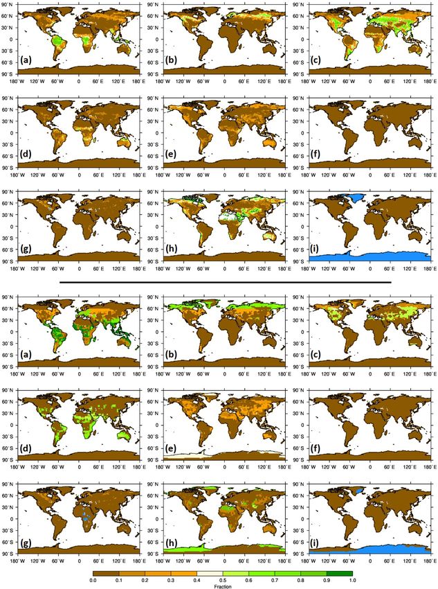
C. J. R. Williams et al.: HadGEM3 simulates a warmer Pliocene than data and other models                                   2141

2     Model and experiment design                                (v) the OASIS3 MCT coupler. All of the above individual
                                                                 components are summarised by Williams et al. (2017) and
2.1    Naming conventions and terminology                        detailed individually by a suite of companion papers (see
                                                                 Walters et al., 2019, for GA7 and GL7; Storkey et al., 2018,
Consistent with CMIP nomenclature, when the simulation is        for GO6; and Ridley et al., 2018, for GSI8). A summary of
spinning up towards atmospheric and oceanic equilibrium,         the major changes in HadGEM3 and their impacts on the
with initially incomplete boundary conditions, it is referred    climate, relative to its most recent predecessor (HadGEM2),
to as the “Spin-up phase” and is only briefly presented here.    are given in Williams et al. (2020b). Here, the mPWP
In contrast, once all required boundary conditions were im-      simulation was run on NEXCS, which is a component of
plemented, the results themselves are taken from the end         the Cray XC40 located at the UK Met Office. NEXCS is
of the simulation, referred to here as the “Production run”.     a partition of the UK Met Office’s platform, Monsoon, on
Here, results are based on the final 50-year climatology of      which the piControl simulation was run, thereby avoiding
this production run. Concerning geological intervals, the pre-   the potential caveat discussed in Williams et al. (2020b)
industrial period and mid-Pliocene Warm Period are referred      concerning different computing platforms.
to as the PI and Pliocene, respectively. In contrast, concern-      Details of the other models discussed here, namely previ-
ing the model simulations using HadGEM3-GC31-LL, con-            ous generations of the same UK Hadley Centre model and
sistent with CMIP6 they are referred to as the piControl and     all of those included in PlioMIP2, are included in the Sup-
mPWP simulations, respectively. We also make use of the          plement (Sect. S1).
naming convention of Haywood et al. (2016; hereafter ab-
breviated to H16), including the nomenclature Exc (where c
is the concentration of CO2 in ppmv, and x is any boundary       2.3     Full Pliocene experiment design
conditions that are Pliocene as opposed to PI, which can be      For the most part, the mPWP simulation presented here
any or none of o = orography, v = vegetation, and i = ice        follows the protocol given in H16, discussed below. The
sheets). Thus, for example Eov500 would be an experiment         main difference is that we do not modify the land–sea mask
using Pliocene orography and vegetation and with CO2 at          (LSM), due to technical challenges of modifying the ocean
500 ppmv but with pre-industrial ice sheets.                     LSM and coupling it to the atmosphere in this model.

2.2    Model description                                         2.3.1    Greenhouse gas atmospheric concentrations,
                                                                          aerosol emissions and ozone
The model presented here is the Global Coupled (GC) 3.1
configuration of the UK’s physical climate model,                Following H16, atmospheric CO2 concentration was mod-
HadGEM3-GC31-LL, which is the “CMIP6-class” UK                   ified in the mPWP simulation, from 280 to 400 ppmv. All
Met Office physical climate model. The piControl simu-           other greenhouse gases, such as CH4 , N2 O and O2 , were
lation for this model was conducted elsewhere as part of         kept as in the piControl simulation. Likewise, aerosol emis-
CMIP6 and is used here for comparative purposes; see             sions (e.g. organic- and black-carbon fossil fuels) and their
Williams et al. (2017), Kuhlbrodt et al. (2018) and Menary       resulting oxidants were kept as in the piControl simulation,
et al. (2018) for further details on HadGEM3-GC31-LL and         consistent with previous palaeoclimate simulations with this
its piControl simulation. The mPWP simulation presented          model (Williams et al., 2020b).
here was run with identical components to those used in             Under strong surface warming, the thermal tropopause
other CMIP6/PMIP4 simulations using this model, namely           rises. In simulations with prescribed ozone concentration it
the midHolocene and lig127k simulations (Williams et             is important that the thermal tropopause remains below the
al., 2020b). The full title for this configuration is HadGEM3-   ozone tropopause in order to avoid unphysical feedbacks as-
GC31-LL N96ORCA1 UM10.7 NEMO3.6 (hereafter                       sociated with increasing cold point temperature (see, for ex-
referred to as HadGEM3). The model was run using the             ample, Hardiman et al., 2019). For this reason, ozone from
Unified Model (UM), version 10.7, and included the follow-       the 1pctCO2 simulation of the UK Earth System Model
ing components: (i) Global Atmosphere (GA) version 7.1,          (UKESM1; see Sellar et al., 2019), in which CO2 concen-
with an N96 atmospheric spatial resolution (approximately        trations are increased relative to 1850 levels at 1 % yr−1 , was
1.875◦ longitude by 1.25◦ latitude) and 85 vertical levels;      prescribed here. UKESM1 uses the same physical climate
(ii) NEMO ocean version 3.6, including Global Ocean              configuration as HadGEM3 but interactively simulates ozone
(GO) version 6.0 (ORCA1), with an isotropic Mercator             chemistry. The ozone was taken from a 10-year period of this
grid that, despite varying in both meridional and zonal          UKESM1 simulation (years 51–60), during which the mean
directions, has an approximate spatial resolution of 1◦ × 1◦     surface temperature was approximately 2 ◦ C warmer than the
and 75 vertical levels; (iii) Global Sea Ice (GSI) version 8.0   piControl simulation. The value of 2 ◦ C was chosen as a
(GSI8.0); (iv) Global Land (GL) version 7.0, comprising          compromise between raising the ozone tropopause enough
the Joint UK Land Environment Simulator (JULES); and             to avoid inconsistency with the thermal tropopause, without

https://doi.org/10.5194/cp-17-2139-2021                                                     Clim. Past, 17, 2139–2163, 2021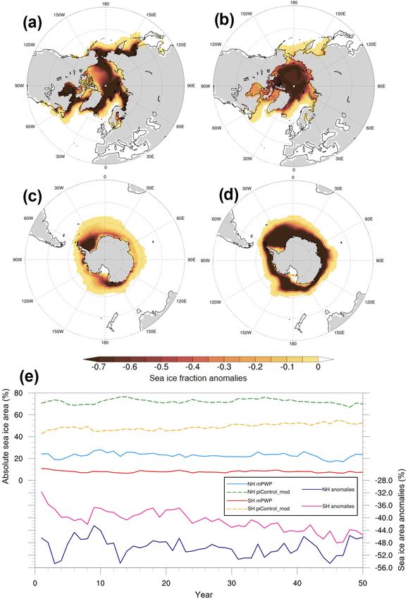
2142                           C. J. R. Williams et al.: HadGEM3 simulates a warmer Pliocene than data and other models

introducing significant changes in ozone forcing relative to       grass and shrubs. In addition to these, there are four non-
the piControl. The impact of the ozone modification could be       vegetated PFTs: urban areas, inland water (or lakes), bare soil
explored in future work, for example by using an ozone pro-        and land ice. This division of grid box into PFTs is consistent
file from a UKESM1 simulation with a higher mean surface           with both of the model’s predecessors (see the Supplement).
temperature (more consistent with the HadGEM3 Pliocene             With the exception of the urban tile, which was kept as PI to
warming; see Sect. 3) or by using the methodology outlined         be consistent with previous palaeoclimate simulations with
in Hardiman et al. (2019), which was used for the CMIP6            this model (Williams et al., 2020b), all of these PFTs were
Shared Socioeconomic Pathway (SSP) scenario simulations            modified in the mPWP simulation.
with HadGEM3.                                                         The US Geological Survey’s PRISM4 (Dowsett et
                                                                   al., 2016) vegetation reconstruction from Salzmann et
2.3.2   Changes to boundary and initial conditions                 al. (2008) was used, provided as a megabiome reconstruction
                                                                   in PlioMIP2 (H16). This can be seen in Fig. 2, where there
Palaeogeography (including land-sea mask, orography                are 10 listed megabiomes corresponding to those used in Har-
and bathymetry)                                                    rison and Prentice (2003): tropical forest, warm-temperate
The mPWP simulation used an identical LSM to the piCon-            forest, savanna and dry woodland, grassland and dry shrub-
trol simulation that, if necessary, is allowed under the exper-    land, desert, temperate forest, boreal forest, tundra, dry tun-
imental design laid out in H16. This differs from both the         dra, and land ice.
standard and enhanced LSMs provided by H16 (accessible,               In order to translate the megabiomes from PRISM into
with all other required boundary conditions, from the US Ge-       the PFTs used by the model, a lookup table was required.
ological Survey’s PlioMIP2 website, http://geology.er.usgs.        Minimum and maximum bounds for each megabiome were
gov/egpsc/prism/7_pliomip2.html, last access: 29 September         firstly obtained, based on values from Crucifix et al. (2005),
2021), in that in both of these the gateways in the Bering         and then estimates were made for each PFT within these
Sea, the Canadian Archipelago and Hudson Bay are closed,           bounds by mapping the pre-industrial megabiomes onto the
whereas in the HadGEM3 simulations only the Canadian               pre-industrial PFT in HadGEM3; the resulting lookup table
Archipelago (Hudson Bay) gateway is closed and the Bering          is shown in the Supplement (Table S1). In this table, for ex-
Strait is open (see Fig. S1 in the Supplement). Likewise, the      ample, each land grid point with the megabiome “Tropical
bathymetry used here is also identical to the piControl simu-      forest” is divided amongst the model PFTs as 92 % BLT, 5 %
lation for the same reasons.                                       bare soil, 2 % tropical C4 grasses and 1 % shrubs. The re-
   The orography used in the mPWP simulation, however,             sulting nine PFTs used in the mPWP simulation, as well as
does follow the protocol of H16. Here, an anomaly is firstly       those from the original piControl, are shown in Fig. 3. The
created by subtracting the PRISM4 modern orography from            largest fractional increases, relative to the piControl, occur
the PRISM4 Pliocene orography and then, after having been          for broadleaf trees and needleleaf trees (18 % and 5 %, re-
re-gridded to the model’s own resolution, adding this to the       spectively; Fig. 3a and b), and the largest decreases occur for
model’s existing orography (see Sect. 2.3.2 in H16). The re-       temperate C3 grass and land ice (15 % and 5 %, respectively;
sults are shown in Fig. 1, where the PRISM4 anomaly shows          Fig. 3c and i). In regions where there is no obvious match
the largest changes are occurring over Greenland and Antarc-       between the model’s PFTs and the megabiomes, such as over
tica, with smaller changes over the Himalayas, North Amer-         western Antarctica (specified as tundra in the PRISM data),
ica and Africa (Fig. 1a). When added to HadGEM3’s existing         the closest match was provided; in this case, a mix of bare
orography (Fig. 1b), the changes result most obviously in a        soil and shrubs.
lowering of orography over Greenland, western and eastern
Antarctica and a raising of orography over central Antarctica      Vegetation functional types
(Fig. 1c). Due to an early model instability relating to the
steep orographic gradients in western Antarctica, this region      Alongside the vegetation fractions, both the piControl and
was smoothed in the final simulation (Fig. 1c).                    mPWP simulations included two monthly varying vegetation
                                                                   functional types, namely leaf area index (LAI) and canopy
                                                                   height, both of which are associated with each of the five
Vegetation fractions (including urban, lakes and ice)
                                                                   vegetated PFTs. Given that no information was available
As part of its GL configuration, both the piControl and            from the PRISM vegetation reconstruction concerning these
mPWP simulations used the community land surface model             fields, two methods were used to create Pliocene LAI and
(JULES; see Best et al., 2011; Clark et al., 2011; Walters et      canopy height. For LAI, a seasonally and latitudinally vary-
al., 2019). In this land surface model, sub-grid-scale hetero-     ing function was created from the zonal means of the piCon-
geneity is represented by a tile approach (Essery et al., 2003),   trol (Fig. 4) and used to build a new field for the Pliocene,
in which each grid box over land is divided into five veg-         for each month and each PFT (see Fig. 4b and c for an ex-
etated plant functional types (PFTs): broadleaf trees (BLT),       ample of the original piControl and the Pliocene newly cre-
needle-leaved trees (NLT), temperate C3 grass, tropical C4         ated field, respectively, both showing LAI for BLT during

Clim. Past, 17, 2139–2163, 2021                                                      https://doi.org/10.5194/cp-17-2139-2021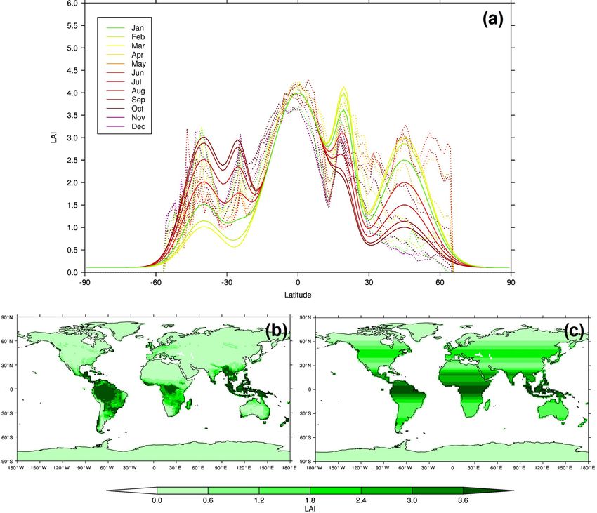
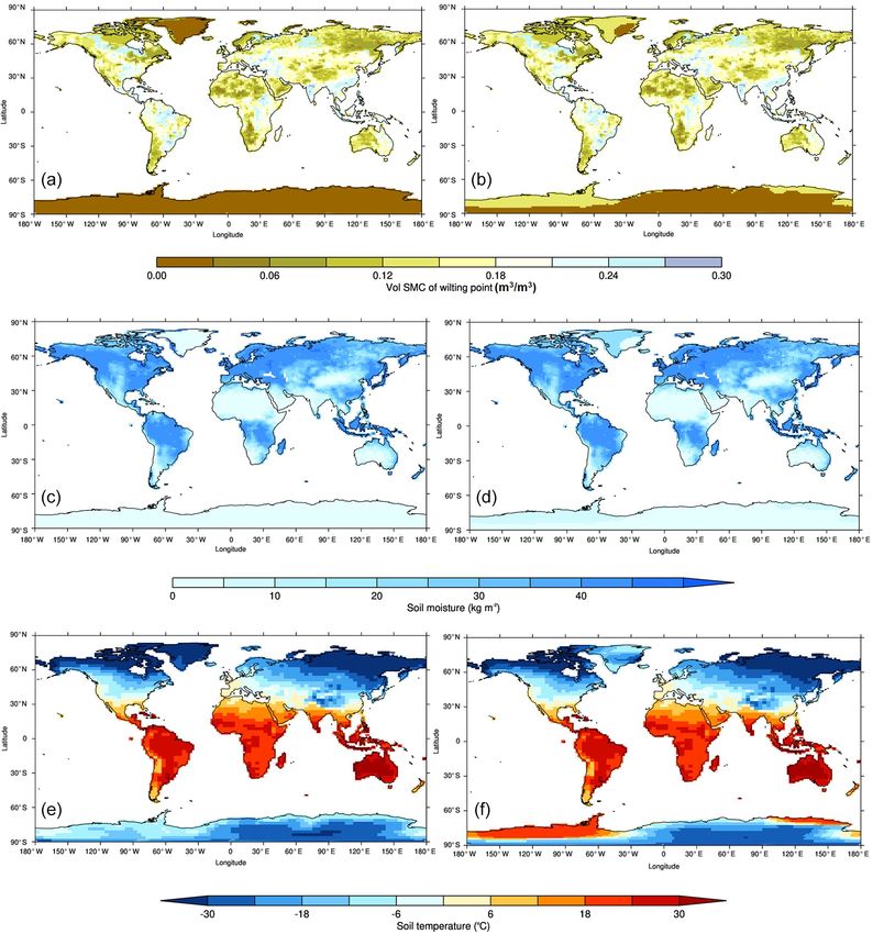
C. J. R. Williams et al.: HadGEM3 simulates a warmer Pliocene than data and other models                                    2143

Figure 1. Changes to topography in HadGEM3 mPWP simulation: (a) PRISM4 anomaly, (b) original field used in the HadGEM3 piControl,
(c) new field used in HadGEM3 mPWP, with smoothed topography over western Antarctica (final version, used in simulation).

Figure 2. The 10 megabiomes from PlioMIP2 used to create the nine PFTs used in HadGEM3 mPWP simulation.

https://doi.org/10.5194/cp-17-2139-2021                                                         Clim. Past, 17, 2139–2163, 2021
2144                             C. J. R. Williams et al.: HadGEM3 simulates a warmer Pliocene than data and other models

Figure 3. The nine PFTs used in HadGEM3. The top half of the figure (the first set of labelled panels) shows the piControl simulation,
and the bottom half shows the mPWP simulation. Values in brackets show global mean differences (mPWP − piControl), expressed as a
percentage: (a) broadleaf trees (18 %), (b) needle-leaved trees (5 %), (c) temperate C3 grass (−15 %), (d) tropical C4 grass (6 %), (e) shrubs
(3 %), (f) urban areas (no change), (g) inland water (1 %), (h) bare soil (−12 %), and (i) land ice (−5 %).

Clim. Past, 17, 2139–2163, 2021                                                               https://doi.org/10.5194/cp-17-2139-2021
C. J. R. Williams et al.: HadGEM3 simulates a warmer Pliocene than data and other models                                    2145

January). This is because LAI varies both in time (i.e. sea-       gradients across western Antarctica; therefore, the field was
sonally) and space in the piControl. Note that although LAI        spatially smoothed so that the gradients were more consis-
does go to zero in the piControl, this was not allowed in the      tent with those in the piControl. Examples of the above soil-
mPWP simulation because the Pliocene does have some veg-           related fields are shown in Fig. 5 for an example month and
etation at high latitudes (see Fig. 3); these functions were       vertical level. A complete list of the soil parameters and soil
therefore increased by x (where x is the mean of the 10 grid       dust properties and how each were changed relative to the
points containing the lowest LAI) such that there is never         piControl are shown in the Supplement (Figs. S3 and S4, re-
zero LAI. In contrast, canopy height in the piControl does not     spectively).
vary monthly and has little variation spatially, and therefore        Outside of the ice regions (i.e. outside Greenland and
canopy height in the mPWP simulation is set to the global          Antarctica), in the mPWP simulation the above soil-related
mean of the piControl simulation (see Fig. S2).                    fields were kept identical to those in the piControl simula-
                                                                   tion.
Soil properties and snow depth

Under newly created land ice based on the new Pliocene ice         2.3.3    Changes to input parameters
mask (i.e. in regions where there is no ice in the piControl       A small number of model input parameters were changed in
simulation but ice in the mPWP simulation), soil parameters,       the mPWP simulation to make the model more stable under
soil dust properties and snow depth were set to be appropriate     the Pliocene boundary conditions. Firstly, a parameter gov-
values for existing ice regions, i.e. whatever these values are    erning the implicit solver for unstable atmospheric bound-
under ice in the piControl simulation are applied to the newly     ary layers was increased, and secondly three parameters for
created ice regions in the mPWP simulation.                        the treatment of canopy snow were made consistent between
   Conversely, and more importantly in this context (as the        BLT and NLT. The same parameter changes will be included
Pliocene represents an overall removal of ice), under newly        in the subsequent version of the physical model (GC4), in or-
exposed land based on the new Pliocene ice mask (i.e. in           der to address occasional model failures that were seen fol-
regions where there is ice in the piControl simulation but         lowing the release of GC3.1. They will be described in more
no ice in the mPWP simulation, primarily over Greenland            detail in a GC4 model documentation paper; however, test-
and western Antarctica), the dominant vegetation fractions         ing of those changes for GC4 has found that they have no
in these regions were firstly identified from the newly cre-       detectable impact on model climatology.
ated Pliocene vegetation. In this case, the dominant fractions
were 40 % shrubs and 60 % bare soil. Following this, grid
points containing this vegetation balance in the piControl         2.4     Modified piControl simulation
were identified, and the soil parameters, soil dust properties
and snow depth values at these points were averaged. This          Given that the official CMIP6 piControl simulation did not
average value, for each of the above fields, was lastly inserted   use the aforementioned model input parameter changes, a
back into the mPWP simulation’s newly exposed grid points;         slightly modified version of this simulation was re-run (sim-
it is acknowledged that this introduces new dust emissions         ulation ID: u-bq637), identical to the piControl other than in-
source regions, which may well impact the resulting Pliocene       cluding the parameter changes outlined in Sect. 2.3.3 (here-
climate state.                                                     after referred to as the piControl_mod simulation). This was
                                                                   run for 200 years, and the last 50-year climatology is consid-
                                                                   ered here in Sects. 3 and 4.
Initial conditions

Oceanic initial conditions, such as ocean temperature and          3     Large-scale features of HadGEM3
salinity, were derived from the mean equilibrium state of the
piControl simulation. Some atmospheric initial conditions,         3.1     Spin-up phase
such as those relating to the land surface (e.g. soil moisture
and soil temperature at four levels of depth), used the same       Consistent with other palaeoclimate model experiments, the
method as that applied to soil properties. These fields con-       simulation should be run for as long as possible to allow the
tain monthly varying values, therefore appropriate timings         model to reach a state of equilibrium before the climatol-
were considered, e.g. if the majority of grid points with the      ogy is calculated over the last 30, 50 or 100 years (Lunt et
above balance were in the Northern Hemisphere, then initial        al., 2017). With this model, however, running for thousands
conditions during Northern Hemisphere summer were used             of years (especially important in obtaining oceanic equilib-
for newly exposed regions in Greenland (and likewise during        rium) was unfeasible given time and resource constraints.
Southern Hemisphere summer for newly exposed regions in            Therefore, by the end of the simulation there was a total of
Antarctica). For the soil temperature field and particularly       576 years for the mPWP simulation, 526 of which are consid-
at upper levels, this process resulted in sharp temperature        ered spin-up, and 50 of which form the final climatologies;

https://doi.org/10.5194/cp-17-2139-2021                                                       Clim. Past, 17, 2139–2163, 2021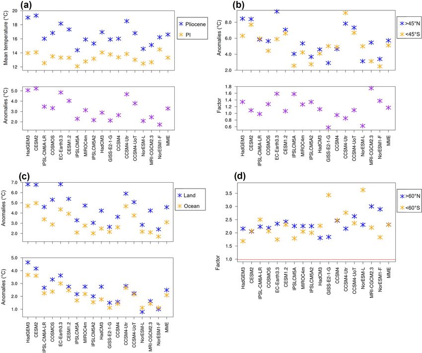
2146 C. J. R. Williams et al.: HadGEM3 simulates a warmer Pliocene than data and other models
Figure 4. LAI used in HadGEM3 for an example PFT (broadleaf trees). (a) Function used to create LAI, where dashed lines show zonal mean
from the piControl simulation and solid lines show seasonally and latitudinally varying function used in the mPWP simulation. (b) Example
of functional types (broadleaf trees, January) used in the piControl simulation. (c) The same as (b) but for the mPWP simulation.
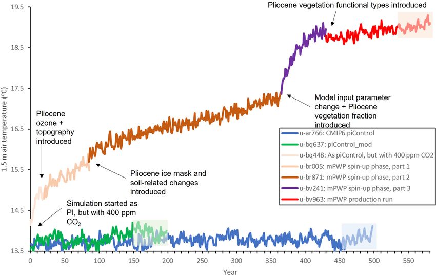
this is approximately consistent with the 652 years of spin-up other than increasing the atmospheric CO2 to 400 ppmv;
used by Menary et al. (2018). identical, therefore, to an E400 experiment following the
naming convention of H16. This ran for ∼ 20 model years,
Evolution of mPWP simulation before branching off to a new suite (u-br005) and introducing
atmospheric ozone appropriate for Pliocene conditions and
The HadGEM3 mPWP simulation was run in multiple parts, Pliocene orography (see Sect. 2.3.1 and 2.3.2, respectively).
each starting from the endpoint of the last, and each introduc- This ran for ∼ 60 model years, before branching off to a new
ing additional boundary conditions so as to gradually move suite (u-br871) and introducing a Pliocene-appropriate ice
from PI conditions to full Pliocene conditions. The mPWP mask along with appropriate values for soil parameters, soil
simulation was started from the endpoint of the CMIP6 pi- dust, soil moisture, soil temperatures and snow depth over
Control simulation, specifically the last part of its spin-up these newly created ice regions (see Sect. 2.3.2); this, there-
phase (u-aq853), consistent with other CMIP6 HadGEM3 fore would be the Eoi400 experiment following the naming
palaeoclimate simulations such as those of the mid-Holocene convention of H16. It should be noted, however, that at this
and Last Interglacial periods (see Williams et al., 2020b). The stage this naming convention is not strictly consistent with
evolution of the mPWP simulation is shown in Fig. 6, where that used by H16 because they specify that orography, lakes
each stage is labelled and the resulting impact on the global and soils should be modified in unison, and therefore “o”
mean 1.5 m air temperature is shown. The first part of the here signifies changes to orography, bathymetry, land–sea
mPWP simulation (u-bq448) is a straight copy of the CMIP6 mask, lakes and soils together. In contrast, at this stage of the
piControl production run (u-ar766), with no modifications
Clim. Past, 17, 2139–2163, 2021 https://doi.org/10.5194/cp-17-2139-2021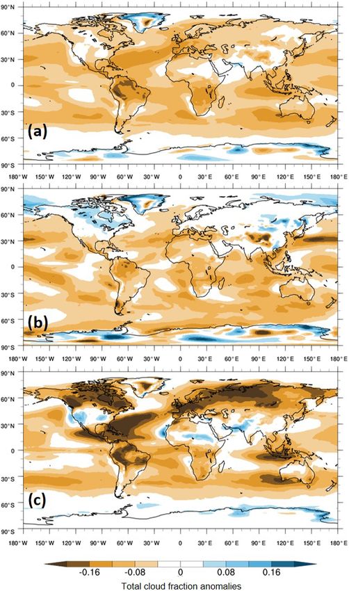
C. J. R. Williams et al.: HadGEM3 simulates a warmer Pliocene than data and other models                                           2147

Figure 5. Example of soil-related fields used in HadGEM3 in the (a, c, e) piControl simulation and (b, d, f) mPWP simulation: (a, b) soil
parameters (example shows volumetric soil moisture content at wilting point), (c, d) soil moisture (example shows January, top level) and
(e, f) soil temperature (example shows January, top level). A complete list of fields is shown in Figs. S3 and S4.

simulation, most boundary conditions are consistent with the           tional types were introduced. This ran for ∼ 150 years, with
experimental design of H16, except vegetation, soils in non-           the final climatology (presented here in Sects 3 and 4) being
ice regions and lakes. This ran for ∼ 280 model years (during          taken from the last 50 years, i.e. allowing a 100-year buffer
which time the task of creating appropriate Pliocene vegeta-           between the final update to the model and the actual results.
tion was completed), before branching off to a new suite (u-              As well as the various stages of the mPWP simulation,
bv241) and introducing a minor parameter change to allow               Fig. 6 also shows time series from the official ∼ 500-year
inclusion of the Pliocene vegetation (see Sect. 2.3.3), as well        CMIP6 piControl simulation (Kuhlbrodt et al., 2018; Menary
as the full Pliocene vegetation fractions. This ran for a further      et al., 2018) and the 200-year piControl_mod conducted here,
∼ 60 years to check the stability of the model in response to          and Fig. S7 shows climatologies of 1.5 m temperature and
the vegetation change, before branching off to a new and final         surface precipitation calculated over the last 50 years of each
suite (u-bv963), in which the full Pliocene vegetation func-           simulation. As the figures show, there is little or no differ-

https://doi.org/10.5194/cp-17-2139-2021                                                            Clim. Past, 17, 2139–2163, 2021
2148                            C. J. R. Williams et al.: HadGEM3 simulates a warmer Pliocene than data and other models

Figure 6. Annual global mean 1.5 m air temperature from the HadGEM3 mPWP spin-up phase and production run, as well as the CMIP6
piControl and the piControl_mod. Labels show introduction of each new Pliocene element. Climatologies discussed here are taken from
final 50 years of each simulation (shown by shaded boxes). See Williams et al. (2020b) for the piControl spin-up phase that preceded these
simulations.

ence between the two PI simulations (also suggested above              in Fig. S6, show the majority of the warming occurring over
in Sect. 2.3.3); using temperature as an example, over the             high-latitude regions in both hemispheres, related to the re-
last 50 years of the simulations there is a mean of 13.79 and          moval of the ice sheets and sea ice loss. By the end of
13.97 ◦ C for the piControl and piControl_mod, respectively,           the mPWP simulation, the mean TOA radiation balance is
and a standard deviation of 0.13 ◦ C for both, further confirm-        0.88 W m−2 , significantly higher than either of the PI simu-
ing the negligible impact of the model parameter change in             lations, suggesting that the mPWP simulation is not yet in full
the model climatology.                                                 atmospheric equilibrium. This TOA imbalance is reducing at
                                                                       a rate of 0.17 W m−2 per century at the end of the simulation.
                                                                       A brief discussion of how the HadGEM3 mPWP simulation’s
3.2    Atmospheric and oceanic equilibrium of the mPWP                 atmospheric equilibrium compares to that of the other Hadley
       simulation                                                      Centre models presented here (introduced in Sect. 4) is given
                                                                       in the Supplement (see Sect. S2 and Table S2).
Concerning atmospheric equilibrium, Table 1 shows sum-                    When the mPWP simulation was stopped, the global
mary statistics for annual global mean 1.5 m air tempera-              annual mean 1.5 m temperature was approximately 19 ◦ C
ture and net top-of-atmosphere (TOA) radiation from the                (Fig. 6). A Gregory plot (Gregory et al., 2004) of the evolu-
last 50 years of the mPWP simulation, compared to both                 tion of TOA energy imbalance and surface temperature can
the piControl and piControl_mod simulations; see Fig. 6 for            indicate how much more warming the model may have expe-
the entire time series of Pliocene 1.5 m air temperature and           rienced if it had been run to full equilibrium. The results of
Fig. S5 for the TOA radiation equivalent.                              this analysis suggest the model would come to equilibrium
   Although the mPWP simulation is clearly warming con-                ∼ 1.5 ◦ C higher (see Fig. S8) at 20.5 ◦ C, i.e. an anomaly rel-
siderably during the ∼ 500-year run (and especially when               ative to the pre-industrial period of 6.6 ◦ C. This is the case
the Pliocene vegetation fraction is introduced), with trends           when the extrapolation is carried out on either of the final
of 0.77 ◦ C per century−1 , it levels off over the final 50 years,     two parts of the simulation (in red and in purple in Fig. S8),
with trends of 0.34 ◦ C per century (Table 1). These values            suggesting that the introduction of the Pliocene vegetation
are higher than those considered by some (e.g. Menary et               functional types does not have a great impact on the final
al., 2018) to be acceptable for equilibrium; however, given            global mean temperature. However, this analysis is associ-
time and resource constraints it was not possible to run the           ated with some uncertainty, related to the interannual vari-
simulation further. The spatial patterns of these trends, shown

Clim. Past, 17, 2139–2163, 2021                                                            https://doi.org/10.5194/cp-17-2139-2021
C. J. R. Williams et al.: HadGEM3 simulates a warmer Pliocene than data and other models 2149
Table 1. Centennial trends (calculated via a linear regression) and climatology over the last 50 years of the simulations. A positive TOA
imbalance indicates a net loss of energy from the Earth system.
Variable piControl piControl_mod mPWP
1.5 m air temperature trends (◦ C per century) 0.51 −0.47 0.34
TOA radiation trends (W m−2 per century) 0.02 −0.2 −0.17
Mean TOA radiation (W m−2 ) 0.18 0.21 0.88
Global ocean volume-mean temperature trends (◦ C per century) 0.03 0.04 0.21
Global ocean volume-mean salinity trends (psu per century) 0.0004 −0.0002 −0.004
ability in temperature and TOA energy imbalance and to the of them are anomalies, i.e. Pliocene − PI. Annual and sea-
fact that the linear extrapolation may not be appropriate if the sonal mean summer/winter 1.5 m air temperature (hereafter
feedbacks vary non-linearly (e.g. Knutti et al., 2015). referred to as near-surface air temperature, SAT) anomalies
As an example of oceanic equilibrium, Table 1 also are shown in Fig. 7. The annual global mean SAT anomaly
shows summary statistics for volume integral annual global for this 50-year climatology is 5.1 ◦ C. Warming relative to
mean ocean temperature and salinity from the end of the the PI is evident throughout the year and globally but more
mPWP simulation compared to both the piControl and pi- so over (i) landmasses (6.8 and 4.5 ◦ C for the annual mean
Control_mod simulations; see Fig. S9 for the Pliocene time SAT over land and ocean, respectively) and (ii) the North-
series. Ocean temperature is steadily increasing throughout ern Hemisphere (8.5 and 6.3 ◦ C for annual mean SAT in the
the mPWP simulation, and likewise ocean salinity is steadily Northern Hemisphere and Southern Hemisphere extratrop-
decreasing (Fig. S9). Freshwater fluxes to the ocean repre- ics; > 45◦ , respectively). Warming is also evident over high
senting iceberg calving and ice sheet basal melt are calibrated latitudes (> 60◦ ) of both hemispheres (10.9 and 8.5 ◦ C for
for the piControl, as described in Sellar et al. (2020). These the Northern Hemisphere and Southern Hemisphere, respec-
fluxes are calibrated to match the ice sheet surface mass bal- tively, and exceeding 12 ◦ C in some places). These partic-
ance (SMB) expected in the piControl, so that salinity drift is ular metrics were chosen to be consistent with those used
minimised. The Pliocene SMB is smaller than that in the pi- by H20 (see Sect. 4.2). Over the tropics (20◦ N–20◦ S) the
Control, and hence net flux of water to the ocean is positive, amount of warming is less than at higher latitudes, but the
leading to the salinity drift. If computational resources al- Pliocene is still much warmer than the PI with annual mean
lowed for a much longer Pliocene simulation, this ocean flux SAT anomalies of 4.6 and 3.7 ◦ C when averaged over trop-
could be calibrated to Pliocene SMB once the temperature ical land and ocean, respectively. This global and regional
and SMB had stabilised or calculated iteratively. The long- warming is consistent with, albeit slightly warmer than,
term trends (Table 1) provide similar conclusions to those other work, namely the results from PlioMIP1 (Haywood et
from the atmospheric trends, for example with centennial al., 2013) and PlioMIP2 (see Sect. 4.2). The majority of the
temperature trends of 0.21 ◦ C per century being much higher annual mean warming (Fig. 7a) in Northern Hemisphere high
than the PI simulations (0.03 and 0.04 ◦ C per century for the latitudes is accounted for during that hemisphere’s winter
piControl and piControl_mod, respectively). Although these (December–February, DJF) with a mean warming of 15 ◦ C
values again do not meet the criteria of Menary et al. (2018) (Fig. 7b), and likewise the majority of the annual mean
for oceanic equilibrium, given the aforementioned computa- warming in Southern Hemisphere high latitudes is accounted
tional cost of this model it was not possible to run the sim- for during that hemisphere’s winter (June–August, JJA) with
ulations further; this is even more true in the ocean, which a mean warming of 10.6 ◦ C (Fig. 7c). If the entire hemisphere
would require many thousands of years of model simula- rather than > 60◦ is considered, then this greater winter con-
tion to reach equilibrium. This compromise has been equally tribution to the annual mean is still true, although the contri-
necessary for other computationally expensive palaeoclimate bution is lower (e.g. 5.6, 6.1, and 5.4 ◦ C for the annual, DJF
simulations (e.g. Williams et al., 2020b). and JJA means, respectively, in the Northern Hemisphere).
The regions of polar SAT increases and seasonal variation
are likely explained by the changes in sea ice shown in Fig. 8
3.3 Simulation comparison: mPWP versus (for the absolute values in sea ice fraction, see Fig. S10). Re-
piControl_mod climatologies ductions in sea ice are shown throughout the year in both
hemispheres, consistent with previous work (e.g. Cronin et
Here the focus is on mean differences between the al., 1993; Howell et al., 2016; Moran et al., 2006; Polyak
HadGEM3 mPWP simulation and its corresponding mod- et al., 2010). Here, although a reduction in sea ice (of up to
ified PI simulation, piControl_mod (Sect. 2.4). All of the 70 %) is evident throughout the year in either hemisphere,
following discussion and figures relate to climatologies cal- at the seasonal timescale the largest loss (exceeding 70 % in
culated over the last 50 years of the simulations, and all
https://doi.org/10.5194/cp-17-2139-2021 Clim. Past, 17, 2139–2163, 20212150 C. J. R. Williams et al.: HadGEM3 simulates a warmer Pliocene than data and other models
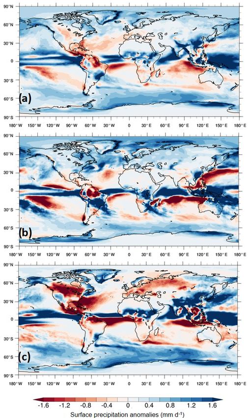
mean precipitation anomaly for this 50-year climatology is
0.34 mm d−1 . In addition to the precipitation increases at
high latitudes at the annual timescale (Fig. 9a), which are
again mostly accounted for by changes during the Northern
Hemisphere’s and Southern Hemisphere’s winters (Fig. 9b
and c, respectively), the largest change relative to the PI
is a northward displacement of the Intertropical Conver-
gence Zone. All timescales are showing wetter conditions
over oceans to the north of the Equator and drier condi-
tions over oceans to the south of the Equator. This is sim-
ilar to work by Li et al. (2018), who suggested a poleward
movement of Northern Hemisphere monsoon precipitation
in PlioMIP1. There is also a noticeable enhancement of mon-
soon systems such as the East Asian and West African mon-
soons, consistent with previous work (e.g. Zhang et al., 2013,
2016). In some places, these changes exceed ∼ 2 mm d−1 ,
geographically consistent with (albeit again much higher
than) other work, such as the multi-model ensemble mean
(MME) from PlioMIP2 models where increases rarely ex-
ceed ∼ 1.2 mm d−1 (see Sect. 4.2). These changes, and in-
deed the temperature changes over Northern Hemisphere
landmasses, may be associated with changes to the total
cloud cover shown in Fig. 10. Although the changes are
small at the annual timescale (Fig. 10a), during Northern
Hemisphere winter (Fig. 10b) there is a noticeable increase
in cloud cover (of ∼ 10 %) over high-latitude regions corre-
sponding to the increases in precipitation. Likewise, during
Northern Hemisphere summer (Fig. 10c) there is a large re-
duction (over 20 % in places) in cloud cover, especially over
Northern Hemisphere landmasses; these regions, such as Eu-
rope and northern Asia, correspond well to the areas of de-
creased precipitation and increased temperature.
4 Comparison of HadGEM3 with other models and
proxy data
Figure 7. The 1.5 m air temperature climatology differences
(mPWP − piControl_mod) from HadGEM3: (a) annual, (b) DJF 4.1 Model–model and model–data comparison: different
and (c) JJA. generations of UK model versus proxy data
Here the focus is on mean SST differences between different
some places, such as the polar Arctic and Antarctic) is seen generations of the UK’s physical climate model, starting with
during each hemisphere’s winter (Fig. 8a and d). The regions three Pliocene simulations using the original fully coupled
and timings of maximum warming (Fig. 7b–c) correspond climate model HadCM3, then a simulation from the more
well to the regions and timings of maximum sea ice loss, im- recent HadGEM2 and finally the mPWP simulation from
plying a role for the sea ice–albedo feedback. When sea ice HadGEM3. See the Supplement for the details of these older
area is averaged over each hemisphere (Fig. 8e), the North- models. For HadCM3, three separate Pliocene simulations
ern Hemisphere is clearly losing more sea ice in the mPWP (and corresponding PIs) are used; the first two were con-
simulation (relative to the piControl_mod) than the Southern ducted by Lunt et al. (2012) and Bragg et al. (2012) and are
Hemisphere. However, the amount of loss in the Southern referred to as HadCM3-PRISM2 and HadCM3-PlioMIP1,
Hemisphere is steadily increasing during the last 50 years of respectively (see Table 2). This is to distinguish them from
the mPWP simulation, suggesting that had the model been a third version of the same model included in PlioMIP2, re-
allowed to run to full equilibrium, the difference between the ferred to here as HadCM3-PlioMIP2.
hemispheres would be reduced. Multi-proxy SST data from the KM5c interglacial com-
Annual and seasonal mean surface daily precipita- piled by McClymont et al. (2020) were used for compara-
tion anomalies are shown in Fig. 9. The annual global tive purposes. Here, they focus on a narrow time slice from
Clim. Past, 17, 2139–2163, 2021 https://doi.org/10.5194/cp-17-2139-2021C. J. R. Williams et al.: HadGEM3 simulates a warmer Pliocene than data and other models 2151
Figure 8. Sea ice fraction climatology differences (mPWP − piControl_mod) from HadGEM3: (a) Northern Hemisphere DJF, (b) Northern
Hemisphere JJA, (c) Southern Hemisphere DJF, (d) Southern Hemisphere JJA and (e) mean sea ice area (both absolute values and differences)
averaged over either hemisphere.
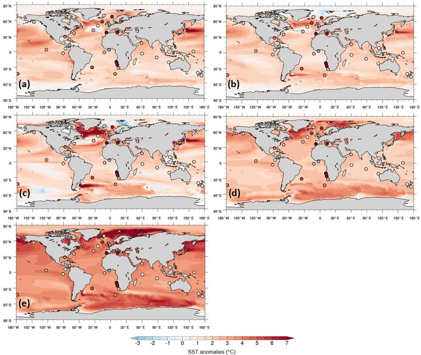
3.195 to 3.215 Ma and compile the SST data from two prox- Maps of annual mean SST anomalies from the simula-
0
ies: an alkenone-derived UK 37 index (Prahl and Wakeham, tions, overlaid with the proxy data, are shown in Fig. 11 and
1987) and foraminifera calcite Mg/Ca (Delaney et al., 1985), summary statistics are shown in Table 3.
with the resulting data comprising the PlioVAR synthesis and The global annual SST anomaly for HadGEM3 is 3.8 ◦ C,
covering 32 locations between 46◦ S–69◦ N (McClymont et followed by HadGEM2 at 2.3 ◦ C and 1.7, 1.5, and 1.6 ◦ C
al., 2020). for the three HadCM3 simulations (starting with the most
recent, HadCM3-PlioMIP2; see Table 3). Comparing the
https://doi.org/10.5194/cp-17-2139-2021 Clim. Past, 17, 2139–2163, 20212152 C. J. R. Williams et al.: HadGEM3 simulates a warmer Pliocene than data and other models
Table 2. Different generations of the UK physical climate model used here and their involvement with PlioMIP.
Model Model name here MIP Boundary conditions Reference
HadCM3 HadCM3-PRISM2 – PRISM2 Lunt et al. (2012)
HadCM3 HadCM3-PlioMIP1 PlioMIP1 PRISM3 Bragg et al. (2012)
HadCM3 HadCM3-PlioMIP2 PlioMIP2 PRISM4 Hunter et al. (2019)
HadGEM2-AO HadGEM2 PlioMIP1 PRISM3 Tindall and Haywood (2020)
HadGEM3-GC31-LL HadGEM3 PlioMIP2 PRISM4 Presented here
Table 3. Global annual mean SST anomalies from Pliocene simulations using different generations of the UK’s physical climate model and
RMSE values between simulations and SST proxy data from McClymont et al. (2020).
HadCM3-PRISM2 HadCM3-PlioMIP1 HadCM3-PlioMIP2 HadGEM2 HadGEM3
Global mean (◦ C) 1.63 1.53 1.67 2.29 3.80
RMSE 3.55 3.62 3.59 3.23 3.36
newest model (HadGEM3) with the oldest model (HadCM3- nor HadGEM3 display (Fig. 11d–e). Where proxy data sug-
PRISM2), which have an anomaly of 3.8 and 1.6 ◦ C, re- gest colder conditions, again none of the models capture the
spectively, clearly the most recent generation shows a much sign of change and all show widespread warming, and this is
warmer Pliocene. most evident in HadGEM3 because of its particularly strong
Comparing an earlier generation of the model with a later warming. The fact that all of the HadCM3 simulations show
generation that has identical boundary conditions (HadCM3- several regions of cooling and have a higher RMSE than the
PlioMIP1 and HadGEM2, respectively; Fig. 11b and d), most recent versions suggests that this early model might be
aside from the greater overall warming (2.3 ◦ C in HadGEM2 too cold. In contrast, the fact that HadGEM3 has a higher
versus 1.5 ◦ C in HadCM3-PlioMIP1) already discussed RMSE than HadGEM2 suggests that, despite involving sig-
above, the main spatial patterns of warming are similar, with nificant model development (see Williams et al., 2020b, for a
both showing the greatest warming over the Labrador Sea summary), concerning Pliocene climate HadGEM3 may ac-
and the northwestern Pacific and HadGEM2 showing greater tually be too warm. Therefore, whilst model development ap-
polar amplification overall. In part thanks to this high-latitude pears to have improved the model’s agreement with proxy
warming, root-mean-squared error (RMSE) values are 3.2 data since earlier versions of the model, this only appears to
and 3.6 ◦ C for HadGEM2 and HadCM3-PlioMIP1, respec- be true up to a certain point; the “sweet spot” appears to be
tively, showing a greater agreement between the proxy data HadGEM2. Moreover, given the aforementioned point about
and HadGEM2 (Table 3). the mPWP simulation not being in full equilibrium and being
Likewise, comparing the other older model with the ∼ 1.5 ◦ C warmer if it had been (see Sect. 3.1.2), it is likely
most recent (HadCM3-PlioMIP2 and HadGEM3, respec- that both the SST anomaly and the RMSE values would be
tively; Fig. 11c and e), the spatial patterns of warming dif- higher when in equilibrium, and therefore the performance
fer more widely, with HadGEM3 showing widespread North- against proxy data may be lower than indicated here.
ern Hemisphere high-latitude warming that is not shown by
HadCM3-PlioMIP2 at all (other than in the Labrador Sea). 4.2 Model–model comparison: HadGEM3 versus
HadGEM3, and indeed HadGEM2, are displaying a greater PlioMIP2 models
extent of polar amplification in both hemispheres (Fig. 11d–
e). As the warmest model, HadGEM3 (RMSE = 3.4 ◦ C) Finally, the focus here is on mean differences, again consid-
shows less agreement with the proxy data than HadGEM2 ering SAT and precipitation anomalies, between the mPWP
(RMSE = 3.2 ◦ C), likely because it is so warm that the dis- simulation from HadGEM3 and the Pliocene simulations
crepancy with the colder proxy data locations (such as in the from all other available models included in PlioMIP2 (Ta-
Indian Ocean, near New Zealand or off equatorial Africa) ble 4).
is greater (Fig. 11e). This is in spite of the fact that in the A number of different metrics of SAT are shown in Fig. 12
warmer proxy data locations (such as in the North Atlantic for each of the models, as well as the MME; the panels shown
and Arctic) HadGEM3 is closer to the proxy data. In these here are updated versions of those shown in H20 but now in-
regions, the earlier versions of the model (Fig. 11a–c) do not cluding HadGEM3. It should be noted that, consistent with
even capture the sign of change and show a weak cooling, H20, the models are listed according to their published ECS,
in stark contrast to the proxy data, that neither HadGEM2 with the highest ECS listed first (see Table 4). HadGEM3
has an ECS of 5.5 K (Andrews et al., 2019), compared to
Clim. Past, 17, 2139–2163, 2021 https://doi.org/10.5194/cp-17-2139-2021C. J. R. Williams et al.: HadGEM3 simulates a warmer Pliocene than data and other models 2153
Table 4. Climate models included here from PlioMIP2 (see Haywood et al., 2020 for each model’s reference).
Model, and modelling centre responsible for simulation Spatial resolution ECS
(long × lat) (◦ C)
Atmosphere Ocean
CCSM4, National Centre for Atmospheric Research, US 1◦ × 1◦ 1◦ × 1◦ 3.2
CCSM4_Utr, Utrecht University, the Netherlands 2.5◦ × 1.9◦ 1◦ × 1◦ 3.2
CCSM4_UoT, University of Toronto, Canada 1◦ × 1◦ 1◦ × 1◦ 3.2
CESM1.2, National Centre for Atmospheric Research, US 1◦ × 1◦ 1◦ × 1◦ 4.1
CESM2, National Centre for Atmospheric Research, US 1◦ × 1◦ 1◦ × 1◦ 5.3
COSMOS, Alfred Wagner Institute, Germany 3.75◦ × 3.75◦ 3.0◦ × 1.8◦ 4.7
EC-Earth3.3, Stockholm University, Sweden 1.125◦ × 1.125◦ 1◦ × 1◦ 4.3
GISS-E2-1-G, Goddard Institute for Space Studies, US 2.0◦ × 2.5◦ 1.0◦ × 1.25◦ 3.3
HadCM3, University of Leeds, UK 2.5◦ × 3.75◦ 1.25◦ × 1.25◦ 3.5
IPSLCM5A, Laboratoire des Sciences du Climat et de l’Environnement, France 3.75◦ × 1.9◦ 2.0◦ × 2.0◦ 4.1
IPSLCM5A2, Laboratoire des Sciences du Climat et de l’Environnement, France 3.75◦ × 1.9◦ 2.0◦ × 2.0◦ 3.6
IPSL-CM6A-LR, Laboratoire des Sciences du Climat et de l’Environnement, France 2.5◦ × 1.26◦ 1.0◦ × 1.0◦ 4.8
MIROC4m, University of Tokyo, Japan 2.8◦ × 2.8◦ 1.4◦ × 1.4◦ 3.9
MRI-CGCM2.3, University of Tsukuba, Japan 2.8◦ × 2.8◦ 2.0◦ × 2.0◦ 2.8
NorESM-L, Bjerknes Centre for Climate Research, Norway 3.75◦ × 3.75◦ 3.0◦ × 3.0◦ 3.1
NorESM-F, Bjerknes Centre for Climate Research, Norway 1.9◦ × 2.5◦ 1.0◦ × 1.0◦ 2.3
the second highest model (CESM2) with an ECS of 5.3 K was 0.09 to 0.18 mm d−1 (Haywood et al., 2013), during
(H20). If, however, all available models within CMIP6 (i.e. PlioMIP2 it was 0.07 to 0.37 mm d−1 (with the higher values
not just those having conducted Pliocene simulations) are being attributed to the models being more sensitive to the
considered, then HadGEM3 has the second highest ECS, just updated PRISM4 boundary conditions), and the PlioMIP2
below that of CanESM5 with an ECS of 5.6 K (Zelinka et ensemble mean was 0.19 mm d−1 (H20). Concerning the
al., 2020). mean, it is the wettest model in terms of both its mPWP
As mentioned above (Sect. 3.2), the global annual SAT (3.49 mm d−1 ) and piControl_mod (3.15 mm d−1 ) simula-
anomaly by the end of the mPWP simulation is 5.1 ◦ C, mak- tions, and both of these are much higher than the MME
ing HadGEM3 one of the warmest models in PlioMIP2 and (3.06 and 2.86 mm d−1 for the Pliocene and PI simulations,
second only to CESM2 (H20). This is true both in terms respectively). The fact that both the HadGEM3 mPWP and
of its anomaly and its mean Pliocene SAT (19 ◦ C); this is piControl_mod simulations are not only the wettest but also
only lagging behind the warmest model by 0.2 and 0.3 ◦ C closer together in terms of mean precipitation, means that
for the anomalous and mean SAT, respectively (Fig. 12a). if the anomaly is considered (Fig. 13b) HadGEM3 does not
HadGEM3 is much warmer than earlier global annual mean quite show the greatest change relative to the PI; an anomaly
temperature estimates (e.g. Haywood and Valdes, 2004), of 0.34 mm d−1 makes it second only to CCSM4-Utr (at
and the range given by models included in PlioMIP1 (1.8 0.37 mm d−1 ). The impact of including HadGEM3 amongst
to 3.6 ◦ C; see Haywood et al., 2013) and PlioMIP2 (1.7 the other PlioMIP2 models is to again slightly increase the
to 5.2 ◦ C, see H20). The impact of including HadGEM3 MME anomaly, from 0.19 mm d−1 as reported by H20 to
amongst the models is to increase the MME anomaly by 0.2 mm d −1 here.
0.1 ◦ C, from 3.2 to 3.3 ◦ C. Interestingly, the HadGEM3 pi- If the hydrological sensitivity (i.e. the relationship be-
Control_mod simulation does not present the warmest ab- tween global annual mean precipitation anomalies and SAT
solute PI compared to the other models, coming fourth in anomalies) of the models is considered, then in line with cur-
the list, suggesting that HadGEM3 is more sensitive to the rent understanding (e.g. Pendergrass and Hartmann, 2014)
Pliocene boundary conditions rather than being a generally there is a clear linear relationship shown by most of the mod-
warmer model overall. els, with Pliocene increases in precipitation increasing in line
Concerning annual global mean precipitation (Fig. 13a), with SAT increases (Fig. 14). This relationship is not entirely
as mentioned above the precipitation anomaly by the end linear, however, with the aforementioned result being shown
of the simulation is 0.34 mm d−1 , making HadGEM3 not again here, i.e. although the HadGEM3 mPWP simulation is
only one of the warmest models in PlioMIP2 but also one of the second warmest of all models in PlioMIP2, it is not the
the wettest (consistent with current understanding, as global wettest, suggesting that although the model is highly sensi-
precipitation is generally a function of global temperature). tive to the Pliocene forcings in terms of its temperature re-
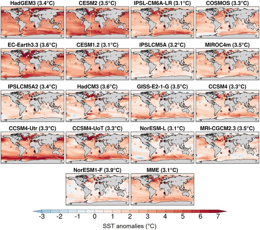
The range of anomalies across all models during PlioMIP1
https://doi.org/10.5194/cp-17-2139-2021 Clim. Past, 17, 2139–2163, 20212154 C. J. R. Williams et al.: HadGEM3 simulates a warmer Pliocene than data and other models Figure 9. Surface precipitation climatology differences Figure 10. Total cloud fraction climatology differences (mPWP − piControl_mod) from HadGEM3: (a) annual, (b) DJF (mPWP − piControl_mod) from HadGEM3: (a) annual, (b) DJF and (c) JJA. and (c) JJA. sponse, it may be less sensitive in terms of its hydrological response. to the MME of 5.1 ◦ C (Fig. 12b, top panel). This is further Returning to SAT and if only extratropical warming (sep- demonstrated by Fig. 12b (bottom panel), showing the ra- arated by hemisphere, above or below 45◦ N or S) is con- tio of warming between the hemispheres (calculated by di- sidered, then HadGEM3 agrees with the other 11 models viding the Northern Hemisphere warming by the Southern (out of 16) that H20 identified as showing enhanced North- Hemisphere warming), where HadGEM3 is giving a ratio ern Hemisphere warming, relative to the Southern Hemi- of 1.34, which is again close to many of the other models sphere (Fig. 12b, top panel). In the Northern Hemisphere, and the MME (1.17). Considering land–sea temperature con- HadGEM3 is again one of the warmest models and (at trasts (Fig. 12c), as H20 state all of the PlioMIP2 models 8.46 ◦ C) is considerably warmer than most other models and show more warming over land both globally and across the the MME; this, with the inclusion of HadGEM3, has now tropics (defined as 20◦ N–20◦ S), and HadGEM3 is no excep- increased from the 5.5 ◦ C reported in H20 to 5.7 ◦ C here. tion. Indeed, over either land or sea, HadGEM3 is the second However, in the Southern Hemisphere HadGEM3 is closer warmest globally and warmest across the tropics, and the in- to many of the other models, although it is still in the top clusion of this model increases the MME by 0.1–0.14 ◦ C de- 33 % of them and with a warming of 6.3 ◦ C is much closer pending on whether land or sea warming is considered. Clim. Past, 17, 2139–2163, 2021 https://doi.org/10.5194/cp-17-2139-2021
You can also read