Representation by two climate models of the dynamical and diabatic processes involved in the development of an explosively deepening cyclone ...
←
→
Page content transcription
If your browser does not render page correctly, please read the page content below
Weather Clim. Dynam., 2, 233–253, 2021
https://doi.org/10.5194/wcd-2-233-2021
© Author(s) 2021. This work is distributed under
the Creative Commons Attribution 4.0 License.

Representation by two climate models of the dynamical and diabatic
processes involved in the development of an explosively deepening
cyclone during NAWDEX
David L. A. Flack1,a , Gwendal Rivière1 , Ionela Musat1 , Romain Roehrig2 , Sandrine Bony1 , Julien Delanoë3 ,
Quitterie Cazenave3 , and Jacques Pelon3
1 Laboratoire   de Météorologie Dynamique/IPSL, Ecole Normale Supérieure, PSL Research University,
Sorbonne University, École Polytechnique, IP Paris, CNRS, Paris, France
2 CNRM, Université de Toulouse, Météo-France, CNRS, Toulouse, France
3 LATMOS-IPSL, CNRS/INSU, University of Versailles, Guyancourt, France
a current affiliation: Met Office, Exeter, UK

Correspondence: Gwendal Rivière (griviere@lmd.ens.fr)

Received: 4 September 2020 – Discussion started: 30 September 2020
Revised: 28 January 2021 – Accepted: 12 February 2021 – Published: 22 March 2021

Abstract. The dynamical and microphysical properties of a        airborne remote-sensing measurements. There is an under-
well-observed cyclone from the North Atlantic Waveguide          estimation of the ice water content in the model compared
and Downstream Impact Experiment (NAWDEX), called the            to the one retrieved from radar-lidar measurements. Consis-
Stalactite cyclone and corresponding to intensive observa-       tent with the increased heating rate in LMDZ6A compared
tion period 6, is examined using two atmospheric compo-          to ARPEGE-Climat 6.3, the sum of liquid and ice water con-
nents (ARPEGE-Climat 6.3 and LMDZ6A) of the global cli-          tents is higher in LMDZ6A than ARPEGE-Climat 6.3 and,
mate models CNRM-CM6-1 and IPSL-CM6A, respectively.              in that sense, LMDZ6A is closer to the observations. How-
The hindcasts are performed in “weather forecast mode”, run      ever, LMDZ6A strongly overestimates the fraction of super-
at approximately 150–200 km (low resolution, LR) and ap-         cooled liquid compared to the observations by a factor of ap-
proximately 50 km (high resolution, HR) grid spacings, and       proximately 50.
initialised during the initiation stage of the cyclone. Cyclo-
genesis results from the merging of two relative vorticity
maxima at low levels: one associated with a diabatic Rossby
vortex (DRV) and the other initiated by baroclinic interac-      1   Introduction
tion with a pre-existing upper-level potential vorticity (PV)
cut-off. All hindcasts produce (to some extent) a DRV. How-      Extratropical cyclones are one of the leading hazards in the
ever, the second vorticity maximum is almost absent in LR        mid-latitudes, but their projected behaviour under climate
hindcasts because of an underestimated upper-level PV cut-       change remains uncertain (e.g. Harvey et al., 2012). This un-
off. The evolution of the cyclone is examined via the quasi-     certainty lies in the location of the extratropical cyclones and
geostrophic ω equation which separates the diabatic heat-        the intensity and position of the storm track (e.g. McDonald,
ing component from the dynamical one. In contrast to some        2011; Zappa et al., 2013b) rather than in the total number
previous studies, there is no change in the relative impor-      of extratropical cyclones (e.g. Finnis et al., 2007; Bengtsson
tance of diabatic heating with increased resolution. The anal-   et al., 2009; Catto et al., 2011; Zappa et al., 2013b).
ysis shows that LMDZ6A produces stronger diabatic heat-             Uncertainties in climate simulations can arise from three
ing compared to ARPEGE-Climat 6.3. Hindcasts initialised         different factors: model physics, internal variability, and
during the mature stage of the cyclone are compared with         forcings (e.g. Hawkins and Sutton, 2009). Therefore, to de-
                                                                 termine confidence in future projections, the historical model

Published by Copernicus Publications on behalf of the European Geosciences Union.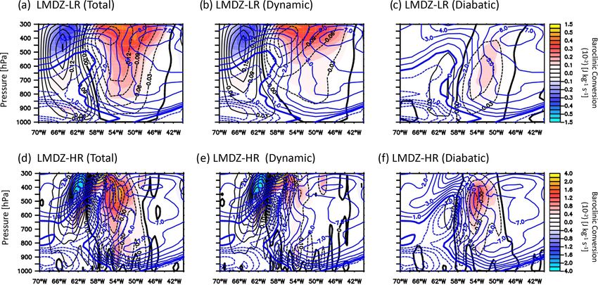
234                                                                     D. L. A. Flack et al.: NAWDEX IOP 6 in two GCMs

climate is compared to observations or re-analyses (e.g.           tural vs. parameter sensitivities (e.g. Sexton et al., 2019; Kar-
Seiler and Zwiers, 2016). Typically, the representation of cy-     malkar et al., 2019).
clones in climate models is considered through statistics, e.g.       The T-AMIP type experiments can also be used as a
number and frequency (e.g. Zappa et al., 2013a; Seiler and         powerful tool for considering the representation of dynam-
Zwiers, 2016). These studies generally indicate systematic         ical processes in climate models. For example, Trzeciak
limitations of coarse-resolution models rarely producing ex-       et al. (2016) showed that climate models of resolution T127
plosively deepening cyclones, producing too many weak cy-          (ca. 1.1–1.5◦ at mid-latitudes) can represent deep extratrop-
clones, and a storm track that is both too zonal and too far       ical cyclones and their tracks well. This good representa-
south.                                                             tion was attributed to an increased importance of the diabatic
   Recently, studies have started to investigate the 3D struc-     heating compared to lower-resolution simulations. Like Trze-
ture of cyclones (e.g. Catto et al., 2010) and the roles of di-    ciak et al. (2016), we consider the dynamical representation
abatic heating in climate models (e.g. Willison et al., 2013;      of extratropical cyclones and the impact of resolution in cli-
Trzeciak et al., 2016; Sinclair et al., 2020). Willison et al.     mate models. However, we focus on a single, well-observed
(2013) and Trzeciak et al. (2016) showed that increased res-       cyclone during the intensive observation period (IOP) 6 of
olution, compared to that of the Coupled Model Intercom-           the North Atlantic Waveguide and Downstream Impact Ex-
parison Project (CMIP) models at the time (CMIP5), was             periment (NAWDEX) field campaign (Schäfler et al., 2018),
required to improve the representation of the diabatic heat-       which is called the “Stalactite” cyclone. This cyclone is ini-
ing and hence representation of the cyclone. This improved         tiated from the interaction of two features that occur on sub-
representation of diabatic heating could be important as Sin-      grid scales of current climate models. The main deepen-
clair et al. (2020) indicated that diabatic processes could be-    ing phase is characterised by the interaction of the surface
come more important in a warming climate. However, fun-            cyclone with successive synoptic-scale upper-level troughs.
damental processes linked to extratropical cyclone formation       Here we answer the following questions on the representa-
and development need further investigation in global circu-        tion of the cyclone in climate models to provide further in-
lation models (GCMs). Fundamental processes linked to fac-         sights into whether climate models are producing cyclones
tors such as cyclogenesis and cyclone development are hard         for the correct reasons.
to examine in full-length free-running climate simulations
and could explain a lack of consideration of this to date.           1. How well do climate models represent the two stages of
Therefore, to examine the representation of the physical pro-           the Stalactite cyclone?
cesses in cyclone formation and development, different tech-         2. What are the relative roles of diabatic and dynamic pro-
niques are required. These techniques include running cli-              cesses in the development of the Stalactite cyclone?
mate model configurations in “weather forecast mode” (e.g.
Phillips et al., 2004) or running short ensemble forecasts (e.g.     3. Are there any differences between the two models’ dia-
Wan et al., 2014).                                                      batic processes that are related to microphysical proper-
   The idea of running climate model configurations in                  ties?
“weather forecast mode” culminated in the formation of the
Transpose – Atmospheric Model Intercomparison Project (T-             The NAWDEX field campaign occurred in September–
AMIP) experiments (Williams et al., 2013). The T-AMIP ex-          October 2016 with the aim of making targeted observations
periments are primarily used to assess whether any long-           of processes that numerical atmospheric models poorly rep-
term model biases occur within the first few days of the           resent (Schäfler et al., 2018). These observations would then
simulations. It was hoped that, if these biases formed early       be used to help determine how well the models represent
in the climate simulations, model improvements to reduce           these processes (e.g. Maddison et al., 2019; Oertel et al.,
those biases could be tested with less computational expense       2019). The observations taken during the field campaign al-
(e.g. Williams et al., 2013; Ma et al., 2013). It was fur-         low for an extra question to be asked in this study.
ther thought this application could help disentangle the ori-        4. Can microphysical observations made during the field
gin of the model biases in a more causal way (e.g. Brient               campaign give any useful information about the climate
et al., 2019). The T-AMIP experiments have considered fac-              model’s performance?
tors such as cloud cover behind fronts in extratropical cy-
clones (e.g. Williams et al., 2013); radiative feedbacks (e.g.     To our knowledge, this study is the first time that a climate
Williams et al., 2013; Bony et al., 2013; Fermepin and Bony,       model is compared with flight data taken during a field cam-
2014); 2 m temperature (e.g. Fermepin and Bony, 2014; Ma           paign without nudging analyses into the simulation, and it is
et al., 2014); precipitation (e.g. Ma et al., 2013; Fermepin and   only feasible because of the T-AMIP protocol.
Bony, 2014; Pearson et al., 2015; Li et al., 2018); and stra-        The questions asked here are of particular interest for the
tocumulus (e.g. Brient et al., 2019); and they have been used      Stalactite cyclone as it influences the development of a block-
alongside random-parameter ensembles to determine struc-           ing anticyclone over Scandinavia and marks the transition
                                                                   between a North Atlantic Oscillation (NAO) positive regime

Weather Clim. Dynam., 2, 233–253, 2021                                                 https://doi.org/10.5194/wcd-2-233-2021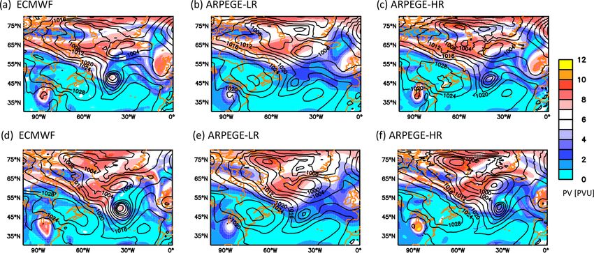
D. L. A. Flack et al.: NAWDEX IOP 6 in two GCMs                                                                                     235

and a Scandinavian blocking regime over the North Atlantic               1 October (Fig. 1a). During the interaction with the second
European sector. Therefore, it is a particularly useful case to          large-scale trough cyclonic wave breaking occurred and the
determine the capabilities of our current climate models.                cyclone re-curved towards Greenland (Fig. 1b). On reach-
   The remainder of this paper has the following layout. The             ing the coast of Greenland cyclolysis (i.e. cyclone decay)
key features of the Stalactite cyclone are discussed in Sect. 2.         occurred; the cyclone had filled in by 00:00 UTC 4 Octo-
The GCMs, experimental set-up, observations, and diagnos-                ber. The cyclone posed an interesting challenge for opera-
tics are described in Sect. 3. The Stalactite cyclone’s repre-           tional numerical weather prediction models as the cyclone
sentation in the two GCMs is discussed in Sect. 4. A sum-                participated in a regime transition from an NAO positive
mary is made in Sect. 5.                                                 regime to a Scandinavian blocking regime which dominated
                                                                         the North Atlantic European sector for the rest of the field
                                                                         campaign (e.g. Schäfler et al., 2018; Maddison et al., 2019).
2   The life cycle of the Stalactite cyclone (NAWDEX                     Correspondingly, there was a reduction in the forecast skill
    IOP 6)                                                               (Schäfler et al., 2018). To determine whether the climate
                                                                         models are correctly simulating the Stalactite cyclone three
The Stalactite cyclone corresponds to IOP 6 of the NAWDEX
                                                                         criteria are developed from its life cycle.
field campaign (Schäfler et al., 2018). It was an explo-
sively deepening cyclone that initially formed at 18:00 UTC                  1. Initial cyclogenesis occurs as a result of the merger of
29 September 2016 (Fig. 1a) off the coast of Newfound-                          a DRV and another near-surface cyclonic vortex associ-
land (ca. 45◦ N, 56◦ W; Fig. 1b). Cyclogenesis occurred as                      ated with baroclinic interaction with an upper-level PV
a result of the merging of two vorticity maxima at low lev-                     cut-off.
els (Fig. 1c). The northern maximum over Newfoundland is
formed via baroclinic interaction with an upper-level poten-                 2. A main deepening phase associated with large-scale
tial vorticity (PV) cut-off that extended down to the surface                   troughs is present.
like a stalactite (hence the name of the cyclone). The southern
                                                                             3. There is a minimum pressure deepening rate of 24 hPa
maximum corresponds to a diabatic Rossby vortex (DRV). A
                                                                                in 24 h during the secondary deepening phase.
DRV corresponds to an isolated positive PV anomaly rapidly
travelling eastward in a moist and baroclinic region1 . To de-           If all of these criteria are met, then the climate models are
termine if this diabatic precursor is a DRV, we use the crite-           able to correctly represent the Stalactite cyclone. The climate
ria set by Boettcher and Wernli (2013). All of the criteria are          models and experimental set-up used are discussed in the fol-
met in ECMWF analysis, which confirms the identification                 lowing section.
of a DRV. It was formed on 27–28 September off the coast
of Florida and South Carolina (not shown). The DRV was
probably produced from a mesoscale convective system, as                 3     Models, observations, and diagnostics
confirmed by satellite images showing cold brightness tem-
perature (e.g. Fig. 1e).                                                 In this section, we discuss the model set-up and experimental
   The two low-level precursors merge into a single cyclonic             protocol of the T-AMIP experiments (Sect. 3.1), the observa-
vorticity maximum in a vortex roll-up by the subsequent                  tions (Sect. 3.2), and diagnostics considered (Sect. 3.3). We
analysis (not shown). The initial cyclogenesis phase led to              also compare our simulations against the European Centre
a short deepening stage over 18 h as the cyclone travelled               for Medium Range Weather Forecasting (ECMWF) analysis
east past Newfoundland. The cyclone underwent a second,                  as a consistent baseline with the initiation state.
more substantial, deepening as a result of an interaction with
                                                                         3.1    Models and experimental set-up
a large-scale region of high PV at upper levels as the cyclone
began to cross the North Atlantic. This region is marked by
                                                                         We use two atmospheric GCMs: ARPEGE-Climat 6.3
multiple regions of high PV (“B” and “C” in Fig. 1d) that are
                                                                         (hereafter ARPEGE) and LMDZ6A (hereafter LMDZ)
successively injected into the upper-level disturbance (“A”)
                                                                         of the CNRM-Cerfacs (Centre National de Recherches
and interact with the Stalactite cyclone. The deepening oc-
                                                                         Météorologiques – Centre Européen de Recherche et de For-
curred at a rate of 24.1 hPa in 24 h and so meets the crite-
                                                                         mation Avancée en Calcul Scientifique; Voldoire et al., 2019)
rion set in Sanders and Gyakum (1980)2 to be classified as
                                                                         and IPSL (Institut Pierre Simon Laplace; Boucher et al.,
an explosively developing cyclone. The explosive deepening
                                                                         2020) climate models: CNRM-CM6-1 and IPSL-CM6A,
occurred between 18:00 UTC 30 September and 18:00 UTC
                                                                         respectively. Both climate models recently contributed to
    1 In essence, this is the same phenomenon as a diabatic Rossby       CMIP6 (Eyring et al., 2016), and here we make use of the
wave (see Appendix of Boettcher and Wernli, 2013).                       same model versions and configurations. Table 1 shows the
   2 A deepening rate of 1 hPa h−1 for 24 h multiplied by                details of the model configurations used. These GCMs are
sin(φ)/sin(60) to adjust to the appropriate latitude to make it equiv-   run in “weather forecast mode” to represent T-AMIP-style
alent to at least 1 bergeron, where φ is the latitude.                   experiments. Hereafter, ARPEGE-LR (-HR) and LMDZ-LR

https://doi.org/10.5194/wcd-2-233-2021                                                      Weather Clim. Dynam., 2, 233–253, 2021
236 D. L. A. Flack et al.: NAWDEX IOP 6 in two GCMs
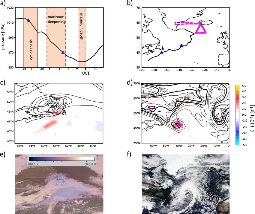
Figure 1. An overview of the Stalactite cyclone. (a) The ECMWF analysis minimum pressure evolution. (b) The track of the Stalactite
cyclone (black). The dashed magenta line is the flight path of SAFIRE Falcon-20 flight 6 and the solid is for flight 7. The star and triangle
in (a) and (b) represent the timing of panels (c) and (e) and (d) and (f), respectively. (c) The ECMWF analysis of the 250 hPa PV > 2 PVU
(contoured) and 850 hPa relative vorticity (shaded) at cyclogenesis (18:00 UTC 29 September), and (d) is like (c) but just before maximum
deepening at 12:00 UTC 1 October. The bold lines are to indicate the PV signature of different PV regions interacting with the cyclone.
“A” is the upper-level signature of the Stalactite cyclone at that time, “B” is the second PV region to interact with the cyclone, and “C” is
the third. The colour scale applies to both (c) and (d). (e) A visible satellite image from MODIS on 29 September indicating the Stalactite
cyclone at cyclogenesis. The brightness temperature has been overlaid and saturated at 50 %. (f) The visible satellite imagery from MODIS
on 1 October 2016. The satellite images are produced by courtesy of NOAA Worldview (https://worldview.earthdata.nasa.gov/, last access:
1 September 2020).
(-HR) refer to low-resolution (high-resolution) runs of the from the centre, resulting in a resolution of approximately
two models. 0.5◦ over the North Atlantic and 1.1◦ elsewhere.
The LMDZ-HR configuration utilises its zoom function, For ARPEGE, microphysics state variables and turbulent
in which the resolution over part of the domain is increased kinetic energy were initialised to zero, and aerosols are pre-
compared to the rest in a variable resolution configuration. scribed from a present-day climatology. On the other hand, in
Here the zoomed domain is centred at 55◦ N, 40◦ E with a the LMDZ model, state variables not defined in the analysis
resolution equivalent to 0.33◦ . The resolution decreases away are set to zero, alongside the aerosols. All hindcasts are per-
formed out to a lead time of T + 10 d. Furthermore, all hind-
Weather Clim. Dynam., 2, 233–253, 2021 https://doi.org/10.5194/wcd-2-233-2021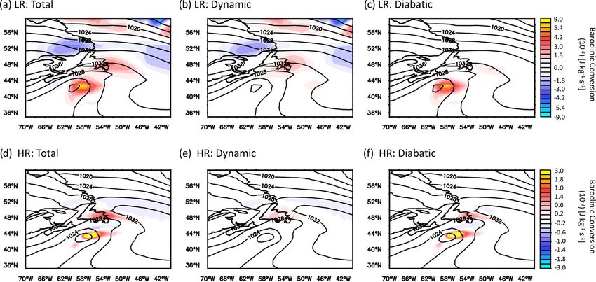
D. L. A. Flack et al.: NAWDEX IOP 6 in two GCMs                                                                                           237

Table 1. Model descriptions with key parameterisations and hindcast resolutions.

                             ARPEGE-Climat 6.3                                        LMDZ6A
                             (Roehrig et al., 2020)                                   (Hourdin et al., 2020)
  Low resolution (LR)        T127 (ca. 150 km globally; output to 1.4◦ )              2.5◦ ×1.2◦
  High resolution (HR)       T359 (ca. 50 km; output to 1.4◦ )                        Zoom function
  Core                       ARPEGE/IFS                                               LMDZ6A
  Vertical levels            91                                                       79
  Convection                 Piriou et al. (2007) and Guérémy (2011)                  Rochetin et al. (2014)
  Long-wave radiation        Mlawer et al. (1997)                                     Mlawer et al. (1997)
  Short-wave radiation       Fouquart and Bonnel (1980); Morcrette et al. (2008)      Extension of Fouquart and Bonnel (1980) to six bands
  Clouds and microphysics    Lopez (2002)                                             Madeleine et al. (2020) and Hourdin et al. (2019)
                                                                                      for low clouds

cast output data are interpolated onto a pressure grid in the              and 1064 nm (e.g. Delanoë et al., 2013). Measurements by
vertical, every 25 hPa, from 1000 to 100 hPa. Output is also               these two instruments allow for the retrieval of ice water
produced using the CFMIP (Cloud Feedback Model Inter-                      content (IWC) thanks to the variational algorithm of De-
comparison Project) Observation Simulator Package (COSP;                   lanoë and Hogan (2008), updated by Cazenave et al. (2019).
Bodas-Salcedo et al., 2011) for radar reflectivities from                  The combination of radar and lidar allows for the identifica-
CloudSat to be compared with the observed aircraft-borne                   tion of the phase of the particles to be identified (e.g. super-
radar reflectivities from the NAWDEX field campaign.                       cooled liquid, ice, liquid, etc.) using principles outlined in
   The hindcasts are initiated at 00:00 UTC 29 September                   Delanoë and Hogan (2010). Furthermore, Doppler-derived
and 1 October 2016 from the ECMWF analysis (including                      wind speeds and radar reflectivities are also used. Retrievals
sea surface and ice cover). The first initiation time is used              from radar products only (RASTA) and a combined radar and
to examine the entire life cycle of the Stalactite cyclone; the            lidar product (RALI) are used to account for uncertainty in
second is used for observational comparisons (Sect. 4.4) to                the measurements. Complementary information on the flight
ensure similar cyclone structure and position to reality. We               and measurements is available in Blanchard et al. (2020).
restrict the number of hindcasts to take into account the im-
pact of the overall synoptic situation at the time being largely           3.3   Vertical motion and baroclinic conversion budgets
unpredictable (e.g. Schäfler et al., 2018). Initial shock (e.g.
Klocke and Rodwell, 2014) is checked for but is not signifi-               Extratropical cyclone evolution can be considered through
cant. However, as a precautionary measure, we do not anal-                 many methods, for example, the surface pressure tendency
yse hindcasts prior to T + 18 h.                                           equation (e.g. Fink et al., 2012); through a potential vorticity
                                                                           framework (e.g. Davis et al., 1993); or the quasi-geostrophic
                                                                           (QG) vertical motion (ω) equation (e.g. Sinclair et al., 2020).
3.2   Observations                                                         Here, as in Sinclair et al. (2020), we consider the evolution
                                                                           through the QG ω equation. We also consider the energetics
During the NAWDEX field campaign, the French SAFIRE                        of the cyclone through the baroclinic conversion (BC).
Falcon aircraft operated from 1–15 October (Schäfler et al.,                  The QG ω equation, which includes diabatic heating and
2018). The SAFIRE Falcon made two flights to observe the                   the β term, can be written in terms of the so-called Q vec-
Stalactite cyclone on 2 October 2016: F6 (towards Green-                   tor following Hoskins et al. (1978) and Hoskins and Ped-
land) and F7 (south of Iceland; Fig. 1b). The second flight                der (1980). We use the formulation of Holton (2004) that in-
(F7) was directly into the cyclone in the ascending branch of              cludes the diabatic heating too:
the associated warm conveyor belt. The first flight (F6) con-
                                                                                       ∂2                         ∂vg
sidered the warm conveyor belt outflow. In the main paper                   σ ∇ 2 + f02     ωQG = −2(∇ · Q) + f0 β
we focus on F7. The first leg of F7 (the most easterly one)                           ∂p 2                         ∂p
was chosen because there was an overpass with CloudSat–                             R 2
                                                                                 −      ∇ J,                                              (1)
CALIPSO track at 14:09 UTC which allows us to assess ob-                           cp p
servation uncertainties by comparing airborne and satellite                for
measurements. The payload on board the SAFIRE Falcon                                 ∂u
included a 95 GHz Doppler cloud radar and a high-spectral-                         R ∂xg · ∇T
                                                                           Q=−       ∂u       ,
resolution Doppler lidar capable of measuring at 355, 532,                         p ∂yg · ∇T

https://doi.org/10.5194/wcd-2-233-2021                                                       Weather Clim. Dynam., 2, 233–253, 2021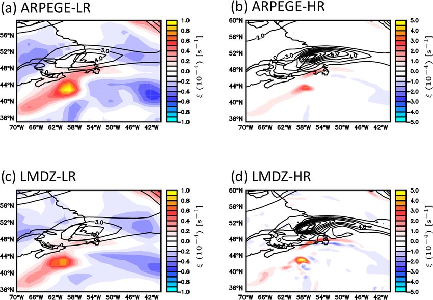
238                                                                       D. L. A. Flack et al.: NAWDEX IOP 6 in two GCMs

where σ is the static stability (obtained by temporally aver-       mum pressure evolution and cyclone track are considered in
aging the temperature across the lifetime of the Stalactite cy-     Sect. 4.1. An in-depth consideration of the cyclogenesis and
clone), f0 is a reference coriolis parameter, β is the beta term    development occur in Sect. 4.2 and 4.3, respectively. The two
in the coriolis forcing, p is the pressure, R is the specific gas   climate models are compared to the flight observations and
constant, cp is the specific heat, J is the rate of heating per     discussed in relation to diabatic heating in Sect. 4.4.
unit mass, ug is the geostrophic wind vector, T is the temper-
ature, x and y are the positions in the meridional and zonal        4.1   Pressure evolution and track
directions, respectively, and ωQG is the vertical velocity ob-
tained from inverting the QG ω equation.                            The representation of the Stalactite cyclone is first considered
   Equation (1) allows us to distinguish between the dynam-         via an overview of the cyclone through its track and mini-
ical and diabatic contributions to the vertical motion in the       mum sea level pressure evolution (Fig. 2). All hindcasts pro-
cyclone. Physically, the Q vector and the β terms represent         duce a rapidly deepening cyclone: slightly more than 24 hPa
the dynamical components of the flow and the Laplacian of           in 24 h in HR hindcasts and slightly less than 24 hPa in 24 h
the rate of heating per unit mass represents the diabatic heat-     in LR hindcasts. However, this deepening is delayed by 24 h
ing.                                                                compared to the analysis in the LR simulations. Furthermore,
   To solve Eq. (1) the 3D Laplacian is inverted over the           the initial cyclogenesis is not as intense in LR simulations
region 35–75◦ N and 70◦ W–0◦ E using Liebmann succes-               compared to the analysis. This weaker cyclogenesis results
sive over-relaxation with boundary conditions such that ω           in an initially weaker cyclone compared to the analysis in
is zero at 1000 hPa, 100 hPa, and all horizontal boundaries.        both models (Fig. 2a). However, the explosive deepening in
The vertical motion is computed every 25 hPa in the vertical.       LMDZ-LR compensates for the lack of initial deepening.
Comparisons of modelled ω and ωQG occur in Sect. 4.3. We            Conversely, ARPEGE-LR has the same secondary deepen-
also invert the dynamic and diabatic components of the ωQG          ing strength as the analysis, so it produces a weaker cyclone.
(ωdyn , ωdiab ) to gain further insights into the development of    The HR hindcasts both have an improved representation of
the cyclone.                                                        the initial cyclogenesis, so they show more realistic cyclone
   Vertical velocity occurs in different key terms of the classi-   development in terms of pressure evolution.
cal equations for the development of extratropical cyclones.           The cyclone track also differs from the analysis. The dif-
We adopt the energetic framework and compute the baro-              ference occurs 18 h after the start of initialisation. The two
clinic conversion from eddy potential energy to eddy kinetic        LR hindcasts produce a track that is too far south and has
energy within the extratropical cyclone (e.g. Orlanski and          a later re-curvature, so the cyclone track occurs further east
Katzfey, 1991; Rivière and Joly, 2006). The baroclinic con-         compared to the analysis and HR hindcasts (Fig. 2b). The
version is proportional to the vertical heat flux and can be        eastward shift in the track agrees with global weather fore-
written as                                                          casts prior to 29 September 2016 (e.g. Maddison et al., 2020).
                                                                    Given the rapid divergence of the forecast track from the
BC = −hω0 θ 0 ,                                                     analysis, differences in the cyclogenesis could be one aspect
                                                                    leading to the track occurring too far east as argued later in
where h = (R/p)(p/ps )R/Cp , ps is the surface pressure, and
                                                                    that section. The cyclogenesis being important for the cy-
θ is the potential temperature. Primes denote the difference
                                                                    clone track is also corroborated by the track representation
from the 5 d temporal average of that quantity centred over
                                                                    having improved (i.e. no eastward shift) after the cyclone ap-
the life cycle of the Stalactite cyclone. The results are insen-
                                                                    pears in the initial conditions (not shown).
sitive to the definition of the temporal average provided it is
                                                                       The main differences to the representation of the Stalactite
made over an interval equal to or longer than the life cycle of
                                                                    cyclone compared to the analysis, on initial inspection, ap-
the cyclone to suppress the cyclone’s signal. The baroclinic
                                                                    pear to be within the cyclogenesis phase of the cyclone and
conversion term is mainly positive in areas following the cy-
                                                                    the different deepening rate of LMDZ compared to ARPEGE
clone trajectory (Rivière and Joly, 2006; Rivière et al., 2015).
                                                                    and the analysis. These two aspects are examined further
   We approximate BC by replacing the vertical velocity by
                                                                    within the following subsections.
its QG formulation in Eq. (1), denoted as ωQG , and keep-
ing θ 0 unchanged. The approximated −hωQG θ 0 is decom-
                                                                    4.2   Cyclogenesis
posed into its dynamic and diabatic components (respec-
tively −hωdyn θ 0 and −hωdiab θ 0 ) by inverting the correspond-
                                                                    The cyclogenesis of the Stalactite cyclone occurs on the
ing components of vertical velocity in Eq. (1) separately.
                                                                    mesoscale as the merging of two low-level vorticity precur-
                                                                    sors: a DRV coming from the subtropics and a vortex lo-
4     Representation of the Stalactite cyclone                      cated further north baroclinically interacting with an upper-
                                                                    level PV cut-off (Fig. 1c). In the present section we anal-
Throughout this section the dynamical and diabatic repre-           yse the representation of the two precursors and their subse-
sentation of the Stalactite cyclone is discussed. The mini-         quent merging in the different simulations. The same vortic-

Weather Clim. Dynam., 2, 233–253, 2021                                                  https://doi.org/10.5194/wcd-2-233-2021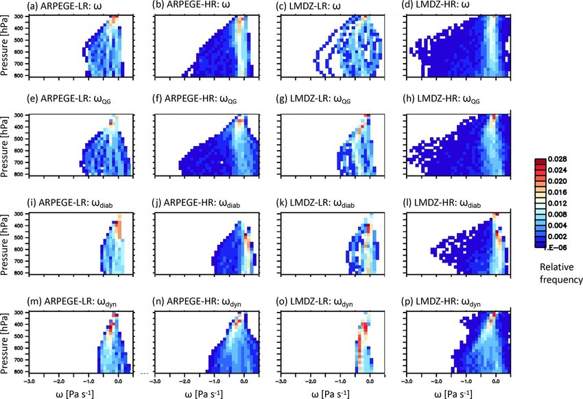
D. L. A. Flack et al.: NAWDEX IOP 6 in two GCMs                                                                                     239

Figure 2. An overview of the Stalactite cyclone: (a) the minimum pressure evolution and (b) the cyclone track. The ECMWF analyses are
in black, LMDZ hindcasts in red, and ARPEGE hindcasts in blue. The LR hindcasts are the solid lines, and the HR hindcasts are dashed. All
hindcasts are initiated at 00:00 UTC 29 September 2016.

ity fields as in Fig. 1c are shown in Fig. 3 for the different         4.2.2   Formation of the northern precursor via
simulations. Figures 4 and 5 show the baroclinic conversion                    baroclinic interaction with the PV cut-off
at T + 18 h for both ARPEGE and LMDZ, respectively, and
help identify the mechanisms behind the two precursors for
the Stalactite cyclone; there is a close relationship between          More important differences appear between LR and HR runs
the two components as the dynamics and diabatic processes              in the representation of the northern precursor. In the LR
are tightly coupled.                                                   hindcasts the vorticity of the northern precursor is much
                                                                       smaller than the vorticity of the DRV precursor (reduced
4.2.1   The diabatic Rossby vortex                                     by factors of 2.4 in ARPEGE-LR and 3.3 in LMDZ-LR),
                                                                       whereas it is only slightly smaller in HR runs (ratio of 1.6
Criteria of DRV introduced by Boettcher and Wernli (2013)              in ARPEGE-HR and 1.3 in LMDZ-HR). Furthermore, the
have been analysed in the different simulations. The two HR            LR runs (Fig. 3a, c) have a more zonal PV cut-off than in the
hindcasts fit all the criteria of a DRV, producing a stronger          analysis (Fig. 1c) and in the two HR runs (Fig. 3b, d). Also,
DRV than the ECMWF, which shows that 50 km grid spac-                  the low-level northern vorticity maximum moves to the east
ing is enough to represent the DRV. The LR hindcasts meet              of the cut-off in the HR runs and analysis, which is typical of
all but two of the criteria of Boettcher and Wernli (2013): the        strong baroclinic interaction, whereas it stays to the south of
PV intensity (for both) and propagation speed (LMDZ-LR;                the cut-off in LR runs (Fig. 3a and c).
Table 2). However, it is encouraging to see that the LR hind-             Unlike the DRV, the northern precursor is a mixture of dia-
casts produce a qualitative representation of a DRV despite            batic and dynamic processes, as shown by the baroclinic con-
the coarse resolution of the models and the mesoscale nature           version rates of Figs. 4 and 5. The vertical cross sections of
of this self-sustaining phenomenon. The identification of the          Fig. 6 show that the dynamical component is mainly centred
southern precursor as a DRV is confirmed by the baroclinic             at upper levels but with an equivalent barotropic structure.
conversion of Figs. 4 and 5 which show that the diabatic com-          This suggests that the northern precursor is forced by the ver-
ponent is almost equal to the total in the vicinity of the vortex      tical velocity associated with the PV cut-off, which is char-
and that the dynamical component is negligible. The DRV                acteristic of type-B cyclogenesis (Petterssen and Smebye,
is more active in LMDZ-LR compared to ARPEGE-LR as                     1971). In LR hindcasts the dynamical forcing has a smaller
the associated heating rate reaches higher values in LMDZ-             vertical extent and is more spread out than the HR hindcasts.
LR compared to ARPEGE-LR (cf. Figs. 4c and 5c). Vertical               The dynamical forcing in LR hindcasts is located further east
cross sections of the heating rates across the DRV indicate            than the diabatic forcing (Fig. 6b and c), while the two forc-
that its structure extends throughout the atmospheric column           ings are more superimposed in HR hindcasts (Fig. 6e and f
(Fig. S1 in the Supplement) confirming the impression left             and Fig. S2 for ARPEGE). Both forcings increase with reso-
by the satellite image (Fig. 1e).                                      lution by a factor of more than 5 in the two models. However,
                                                                       the peak values of the diabatic baroclinic conversion exhibit a
                                                                       larger increase than those of the dynamical baroclinic conver-

https://doi.org/10.5194/wcd-2-233-2021                                                   Weather Clim. Dynam., 2, 233–253, 2021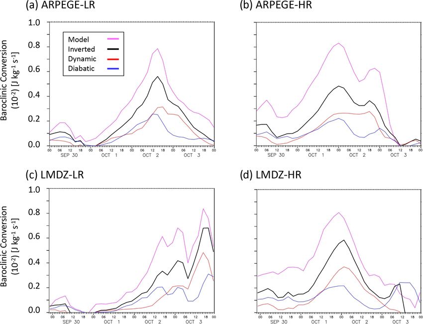
240                                                                           D. L. A. Flack et al.: NAWDEX IOP 6 in two GCMs

Figure 3. Hindcasts for the cyclogenesis of the Stalactite cyclone at 18:00 UTC 29 September (T +18 h) for hindcasts initiated at 00:00 UTC
29 September. The 250 hPa PV above 2 PVU (contoured every 1 PVU) and the 850 hPa relative vorticity (shaded) for (a) ARPEGE-LR,
(b) ARPEGE-HR, (c) LMDZ-LR, and (d) LMDZ-HR. The colour scale is different between LR and HR runs.

Figure 4. Vertically averaged baroclinic conversion between 850 and 300 hPa (shaded) and mean sea level pressure (contoured) at 18:00 UTC
29 September 2016 (T +18 h from hindcast initiation at 00:00 UTC 29 September 2016) for ARPEGE hindcasts. (a–c) ARPEGE-LR hindcast
and (d–f) ARPEGE-HR hindcast. (a, d) Total (dynamic plus diabatic) baroclinic conversion, (b, e) baroclinic conversion from dynamical
processes, and (c, f) baroclinic conversion from diabatic processes. The colour scales refer to each row.

Weather Clim. Dynam., 2, 233–253, 2021                                                       https://doi.org/10.5194/wcd-2-233-2021
D. L. A. Flack et al.: NAWDEX IOP 6 in two GCMs                                                                                          241

Figure 5. As in Fig. 4 but for LMDZ-LR (and -HR) hindcasts.

Table 2. Distance and PV criteria from Boettcher and Wernli (2013) for identifying DRVs between T + 18 and T + 24 from the hindcast
initialised at 00:00 UTC 29 September. The PV criterion is based on a minimum PV value when averaged at the minimum MSLP location and
the eight surrounding grid boxes, which is set to 0.8 PVU. The distance criterion is based on a minimum distance travelled by the vortex in
6 h, which is 250 km. When the threshold is reached a X is present, otherwise a ×. The DRV is described as quantitative if all the thresholds
are reached and qualitative otherwise. Only criteria for which at least one of the hindcasts do not meet the criteria are shown.

  Model              PV (T + 18)     PV (T + 24)     850 hPa PV criterion    Distance     Distance criterion   DRV type
                       (PVU)           (PVU)               (X/×)              (km)             (X/×)           (qualitative or quantitative)
  ECMWF (1.1◦ )          0.94            1.18                  X               370.6              X            Quantitative
  ARPEGE-LR              0.65            0.72                  ×               302.4              X            Qualitative
  ARPEGE-HR              1.45            1.74                  X               328.3              X            Quantitative
  LMDZ-LR                0.51            0.68                  ×               138.6              ×            Qualitative
  LMDZ-HR                2.77            2.54                  X               264.5              X            Quantitative

sion during the formation of the northern precursor (Figs. 5b,           and upper-level dynamical precursor 12–18 h earlier than the
c, e, f and 6b, c, e, f).                                                LR runs (not shown). For LMDZ-LR there is even no merg-
   To conclude, the northern precursor is rather poorly rep-             ing of the two precursors. The delay or absence of interaction
resented in LR compared to HR hindcasts because the less                 between the two precursors likely has an impact on the track
intense, and more spatially diluted, PV inside the cut-off in-           of the cyclone which was systematically located too far east
duces a weaker dynamical forcing. An additional factor is                in the LR runs (Fig. 2b) as the precursor merger starts the
the more active diabatic forcing in HR hindcasts in the vicin-           more northward movement of the cyclone in the track. This is
ity of the northern precursor. So whilst both the dynamical              understandable by the fact that the earlier merging is associ-
and diabatic terms improve with resolution, it is difficult to           ated with a stronger upper-level forcing which is required for
determine which component matters most.                                  a cyclone to move northward perpendicularly to the jet axis
                                                                         (Coronel et al., 2015). There are two factors to explain the de-
4.2.3   Merging of the two precursors                                    layed or missed merging. One is the more rapidly eastward
                                                                         propagation of the DRV in HR than LR runs (Fig. 3; Table 2),
                                                                         which is consistent with stronger latent heating in the former
For the hindcasts shown here, the merger of these two dif-
                                                                         runs. The second is that the low-level northern precursor and
ferent precursors differs in timing from the analysis and be-
                                                                         the upper-level cut-off are moving less rapidly eastward in
tween resolutions. The HR configurations (although delayed
                                                                         HR runs (not shown). This can be partly explained by the
by 6 h compared to the ECMWF analysis) merge the DRV

https://doi.org/10.5194/wcd-2-233-2021                                                      Weather Clim. Dynam., 2, 233–253, 2021
242                                                                            D. L. A. Flack et al.: NAWDEX IOP 6 in two GCMs

Figure 6. A vertical cross section averaged across the northern precursor in the LMDZ hindcasts at 18:00 UTC 29 September 2016 (T +18 h).
The baroclinic conversion (shaded), potential temperature anomaly (blue contours), and inverted ω (black contours) for (a, d) total baroclinic
conversion, (b, e) the baroclinic conversion due to dynamic processes only, and (c, f) the baroclinic conversion from diabatic processes.
(a–c) LMDZ-LR and (d–f) LMDZ-HR. Note that the colour scales and contours are different between the LR and HR runs.

difference in longitude of the dynamical forcing between LR                 In the cyclone average values (Fig. 7) the two stages of
and HR hindcasts (compare Fig. 6b and e). The more rapid                 cyclone development are well separated: (i) the initial cy-
propagation of the DRV and less rapid motion of the north-               clogenesis stage occurring on 29–30 September (Sect. 4.2)
ern precursor explain why the DRV is more able to catch up               and (ii) the main development stage that is dominated by the
to the northern precursor in HR runs as in the analysis.                 presence of a large-scale trough and an explosively devel-
   To conclude on cyclogenesis, the LR hindcasts struggle                oping cyclone. The initiation stage is clearly dominated by
to correctly represent the initiation of the cyclone because             diabatic processes. During the main deepening stage the dy-
they miss the initial deepening of the northern small-scale              namical processes begin to be more important, and more so
low-level vortex and the roll-up of the merging of the two               in the HR hindcasts compared to the LR hindcasts. In the
low-level vortices around the PV cut-off. However, the unex-             HR runs the dynamical term is even larger than the diabatic
pected result is that the LR hindcasts are able to reproduce             term during the whole main deepening stage. The delay in the
the behaviour of the DRV rather well, albeit with a smaller              dynamical processes compared to diabatic processes is par-
propagation speed.                                                       ticularly clear in LR hindcasts, suggesting a delayed forcing
                                                                         by the large-scale upper-level trough. Therefore, there is an
4.3   Main deepening                                                     increased importance of the dynamic term relative to the di-
                                                                         abatic term with increased resolution. This ratio consistency
The main focus of this section is the main deepening stage of            is true for both the maximum (Fig. S3) and average values
the Stalactite cyclone. Like the cyclogenesis phase, the main            (Fig. 7) in both models and lead times. Furthermore, the ra-
deepening phase is considered by analysing the baroclinic                tio consistency in the main deepening stage disagrees with
conversion. The baroclinic conversion is considered either as            the previous studies of Willison et al. (2013) and Trzeciak
an average over a 10◦ × 10◦ area centred on the minimum                  et al. (2016). However, for the northern precursor at cycloge-
pressure of the Stalactite cyclone (Fig. 7) or from its local            nesis we do agree with their studies.
maximum (Fig. S3). The averaged QG baroclinic conversion                    Considering the dynamical processes in more detail
roughly recovers 60 %–70 % of the amplitude of that directly             (Figs. 8 and S4) helps to indicate the reason for the delay in
calculated from the model ω (Fig. 7) throughout the cyclone              the maximum deepening in the LR hindcasts compared to the
life cycle. In addition, the model and QG baroclinic conver-             analysis and the HR hindcasts. On 1 October at 00:00 UTC
sions are very similar in the timing, evolution, structure (not          an upper-level PV signature is clearly visible above the sur-
shown), and maximum peaks (Fig. S3). This good correspon-                face cyclone in HR hindcasts, while in the LR hindcast the
dence provides confidence in our inversions and results.

Weather Clim. Dynam., 2, 233–253, 2021                                                         https://doi.org/10.5194/wcd-2-233-2021
D. L. A. Flack et al.: NAWDEX IOP 6 in two GCMs 243
Figure 7. The evolution of the average baroclinic conversion in a 10 ◦ × 10 ◦ box around the minimum pressure of the Stalactite cyclone for
(a) ARPEGE-LR, (b) ARPEGE-HR, (c) LMDZ-LR, and (d) LMDZ-HR. The magenta line is for the baroclinic conversion calculated with
the model ω, the black line is the total inverted ω, the red line is the inverted ω from dynamical processes, and the blue line is the inverted ω
from diabatic processes. All hindcasts were initiated at 00:00 UTC 29 September 2016, and average times are defined, subtly, differently in
LMDZ and ARPEGE, hence the 1.5 h extension in LMDZ plots. Maximum point values of baroclinic conversion are shown in Fig. S3.
cyclone is still mainly a DRV. The PV injection coming from casts the delay is about 24 h and the eastward shift is more
the large-scale region of high PV, located to the north-east, marked.
into the upper-level disturbance interacting with the surface
cyclone is delayed in the hindcasts. In the analysis some PV 4.4 Interpretation of the difference between the models
injection has already occurred (Fig. 8a) but is just starting in and comparison with aircraft observations
the HR runs (Fig. 8c). The situation in ARPEGE-HR on 1
October at 12:00 UTC (Fig. 8f) resembles more that of the As previously said, to have cyclone features roughly at
analysis approximately 6 h earlier (not shown), with the cy- the same place in the models as in the observations, for a
clonic wave breaking being more advanced in the ECMWF clean comparison, simulations initiated at 00:00 UTC 1 Oc-
analysis (Fig. 8d). Several studies have shown that the PV of tober 2016 are analysed in the present section.
the upper-level trough baroclinically interacting with a sur-
4.4.1 Diabatic heating in the models
face extratropical cyclone tends to advect the cyclone pole-
wards (Rivière et al., 2012; Oruba et al., 2013; Coronel et al., To more deeply investigate the relative contributions of dy-
2015). Therefore, the earlier non-linear interaction of the cy- namics and diabatic components, as well as to assess po-
clone with the large-scale upper-level PV reservoir and the tential differences between the models, Fig. 9 shows distri-
earlier roll-up of the two features around each other explain butions of vertical velocities around the cyclone centre for
the earlier deviation of the cyclone track to the north and the hindcasts initiated at 00:00 UTC 1 October 2016, but sim-
more westward position of the track in the analysis than in ilar results occur for the hindcasts initiated at 00:00 UTC
the hindcasts. For the HR hindcasts the delay is a maximum 29 September 2016 (not shown). Figure 9 first shows that the
of 6 h and the eastward shift is minimal, while for LR hind- distribution of the model ω is rather well represented by its
https://doi.org/10.5194/wcd-2-233-2021 Weather Clim. Dynam., 2, 233–253, 2021244 D. L. A. Flack et al.: NAWDEX IOP 6 in two GCMs Figure 8. The 250 hPa PV (shaded) and mean sea level pressure (contoured) during the maximum deepening phase of the Stalactite cyclone. (a–c) 00:00 UTC 1 October 2016 and (d–f) 12:00 UTC 1 October 2016. (a, d) ECMWF analysis, (b, e) ARPEGE-LR hindcast, and (c, f) ARPEGE-HR hindcast. All hindcasts were initiated at 00:00 UTC 29 September 2016, and the colour scale applies to all plots. LMDZ-LR(- HR) plots at the same time are shown in Fig. S4. Figure 9. Bivariate histograms of vertical velocity vs. pressure in a 6◦ × 6◦ box around the minimum pressure during the mature stage of the cyclone around maximum depth (ca. 12:00 UTC 2 October 2016; T +33–36 h) for (a–d) modelled ω, (e–h) ωQG , (i–l) ωdiab , and (m–p) ωdyn and for (a, e, i, m) ARPEGE-LR, (b, f, j, n) ARPEGE-HR, (c, g, k, o) LMDZ-LR, and (d, h, l, p) LMDZ-HR. The colour scale applies to all plots. The hindcasts were initiated at 00:00 UTC 1 October 2016. Weather Clim. Dynam., 2, 233–253, 2021 https://doi.org/10.5194/wcd-2-233-2021
D. L. A. Flack et al.: NAWDEX IOP 6 in two GCMs 245
QG approximation ωQG (Fig. 9a–d and e–h). Only some peak certainty in the observations, which is useful to be compared
values of model ω near −2 Pa s−1 for LMDZ-LR are miss- with model outputs.
ing in ωQG . Second, both vertical velocities increase with in- The model contribution to Fig. 10 consists of four rows:
creased resolution (Fig. 9a, c, e, g and b, d, f, h). Distribu- the first two rows show “potential” IWC, while the last
tions of ωQG are rather similar in ARPEGE-LR and LMDZ- two show “maximum” IWC. Comparing the first two rows
LR, but the relative contributions of dynamic and diabatic (Fig. 10b–e and g–j) with the observations shows an under-
parts differ between the two runs. There are more frequent estimation of the model IWC. This underestimation is by a
strong ascents of the diabatic component for LMDZ-LR than factor of 3–4, similar to what Rysman et al. (2018) found
ARPEGE-LR (Fig. 9i, k), while the dynamical component when comparing observations and Weather Researching and
partly offsets this difference (Fig. 9m, o). In HR hindcasts, Forecasting (WRF) model simulations of Mediterranean sys-
there are the largest values of ωQG in LMDZ-HR compared tems. Furthermore, the peak of the model IWC distribution
to ARPEGE-HR (Fig. 9f, h) which is mainly due to the dia- occurs at 700–750 hPa, 100–150 hPa lower than in the ob-
batic term. servations. There are small improvements with resolution:
To conclude, diabatic processes have a stronger impact on the HR simulations have a larger IWC throughout, particu-
vertical velocities in LMDZ than ARPEGE, and the diabatic larly aloft and in the maximum values. Furthermore, there
heating in the former model is stronger than in the latter. The are differences between the models. The first difference is
terms that dominate the heating profiles both in ARPEGE that the IWC values of LMDZ-LR are more dispersed than
and LMDZ are the large-scale condensational heating and those of ARPEGE-LR, suggesting a larger number of ice
convective terms (not shown). Thus, it is likely that obser- clouds at this altitude in LMDZ-LR (Figs. 10b, d, g, i; 11a,
vations of microphysical properties of the Stalactite cyclone b). The greater values at upper levels in LMDZ are more in
could be used to qualitatively determine which model has the line with the values given by the observations than ARPEGE
better heating rates or structure. These comparisons are con- (cf. Fig. 10a–j). However, although LMDZ may be better at
sidered next. representing the IWC at upper levels, the overall shape of
the distribution is better in ARPEGE compared to LMDZ.
4.4.2 Microphysical properties in the models and in Indeed, the decreased IWC from 600 to 300 hPa is better
observations represented in ARPEGE. Applying the observation mask to
the models (Fig. 10g–j) brings the frequencies more in line
To determine whether observations of microphysical proper- with the observations compared to those without the mask
ties from field campaign flights can provide information on by removing all the lowest values seen in the no-mask statis-
the underlying diabatic heating, the Stalactite cyclone hind- tics. This is due to instruments not being sensitive to very
casts are compared with flight F7 (Fig. 1b) of the SAFIRE small IWC, and also the models do not create discontinuities
Falcon during the NAWDEX field campaign. To ensure a fair in IWC between cloudy and clear-sky regions. The compar-
comparison, the observation data have been linearly interpo- isons between the mask (Fig. 10g–j) and no-mask (Fig. 10b–
lated onto the model grid, and a nearest-neighbour approach e) values implies that there are very small IWC values in
has been used to convert the model onto the flight track. Ob- the model outside of the observed region (particularly for
served IWC is compared against “potential” IWC (cloud ice ARPEGE-LR), indicating the horizontal structure of the cy-
plus snow) and “maximum” IWC (cloud ice plus snow plus clone is reasonable.
liquid water content, LWC) to take super-cooled liquid into Is the underestimated IWC in the models due to the un-
account. derestimated liquid-to-solid transition for cold temperatures
The wind speeds in the cyclone are well represented in or to the underestimation of condensates as a whole? To an-
all hindcasts with there only being a small shift in the prob- swer this question the LWC below 273 K is added to the IWC
ability density function toward smaller values by less than to create the last two rows (“maximum” IWC; Fig. 10k–r).
5 m s−1 (not shown). This comparison provides confidence Adding the LWC makes limited difference to either of the
in the large-scale features of the cyclone. Therefore, micro- ARPEGE hindcasts (Fig. 10k, l, o, p), suggesting that either
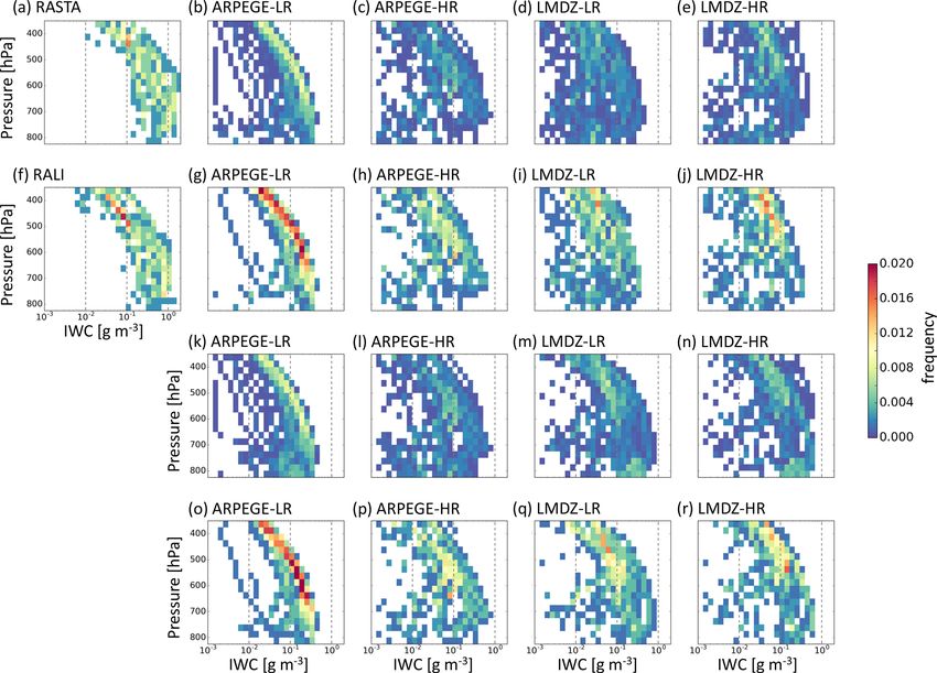
physical features can be further considered. Figure 10 shows there are fewer LWC points added or the LWC points added
bivariate histograms of the IWC for F7 from two observation have a small magnitude. On the other hand, adding LWC into
platforms: RASTA (Fig. 10a) and RALI (Fig. 10f). There the LMDZ definition drastically changes the shape and in-
are larger values of IWC in RASTA compared to RALI be- creases the values of total IWC at lower levels (Fig. 10m, n,
cause the lidar (being sensitive to smaller ice particles and q, r). The LMDZ distributions have been changed to the ex-
smaller quantities of ice) information in RALI leads to a re- tent that the shape now shows more agreement with the ob-
duction of IWC compared to RASTA. Both platforms show servations than when the LWC was not taken into account.
the same shape with increasing values of IWC to around These changes in LMDZ are also apparent in Fig. 11, al-
600 hPa and then a uniform distribution until around 800 hPa, though the model difference is reduced at increased resolu-
below which the instruments no longer detect ice clouds. The tion (Fig. 11c and d). The much larger “maximum” IWC in
two retrieved IWC histograms provide an indication of un-
https://doi.org/10.5194/wcd-2-233-2021 Weather Clim. Dynam., 2, 233–253, 2021246 D. L. A. Flack et al.: NAWDEX IOP 6 in two GCMs Figure 10. Bivariate histograms of ice water content vs. pressure for F7 for (a) RASTA observations (radar only), (f) RALI (radar plus lidar) observations, (b–e) hindcast output using “potential” ice water content (cloud ice plus snow) without applying a mask to the observations, (g–j) hindcast output of “potential” ice water content with the observation mask applied, (k–n) hindcast for “maximum” ice water content (ice water content plus liquid water content) without the observation mask applied, and (o–r) hindcast of “maximum” ice water content with the observation mask applied for (b, g, k, o) ARPEGE-LR, (c, h, l, p) ARPEGE-HR, (d, i, m, q) LMDZ-LR, and (e, j, n, r) LMDZ-HR. The hindcast data are initiated at 00:00 UTC 1 October 2016 and use the nearest grid point to the flight path from the two times surrounding the flight path (12:00 and 15:00 UTC 2 October 2016; T + 36–39 h). The flight occurred from 13:00–16:00 UTC. The colour scale applies to all panels, and the histograms have been normalised by all points. LMDZ compared to ARPEGE over all the levels is consistent are combined with the mixed-phase values. Table 3 shows with the larger diabatic heating shown in Fig. 9e–h. that whilst the combined ice points exceed those of the obser- Given the change by the inclusion of LWC in the def- vations (particularly for ARPEGE) the values are not unrea- inition of the IWC, it is useful to know the proportion of sonable. However, when the combined super-cooled liquid ice, mixed-phase, and super-cooled liquid points that make water is considered, the models significantly overestimate up these distributions. We arbitrarily define ice points in the the amount of super-cooled liquid points by factors of 24– model to be those in which the LWC component of the “max- 47. Considering Table 3 alongside the earlier discussion of imum” IWC is less than 1 % and “pure” super-cooled liquid the impact of adding LWC shows that the super-cooled liq- to be points in which the LWC component is greater than uid water being added to ARPEGE is of a smaller magnitude 99 % of the “maximum” IWC; all other points are mixed than that of LMDZ. It is also worth noting that although the phase. These results are compared with those points defined LR hindcasts are more largely underestimating the IWC than as super-cooled liquid, mixed phase, and ice retrieved IWC the HR hindcasts, they are closer to the observations than the from RALI measurements. To ensure a fair comparison be- HR hindcasts in the percentage of super-cooled water. tween ice and super-cooled liquid water, the “pure” values Weather Clim. Dynam., 2, 233–253, 2021 https://doi.org/10.5194/wcd-2-233-2021
D. L. A. Flack et al.: NAWDEX IOP 6 in two GCMs                                                                                           247

Figure 11. Difference bivariate histograms for F7 of ice water content vs. pressure between ARPEGE and LMDZ for (a) LR differences in
“potential” ice water content (cloud ice plus snow) only (Fig. 10b–d), (b) HR differences in “potential” ice water content only (Fig. 10c–e),
(c) LR differences in “maximum” ice water content (ice water content plus liquid water content) (Fig. 10k–m), and (d) HR differences in
“maximum” ice water content (Fig. 10l–n). Reds refer to ARPEGE having a larger quantity and blues for LMDZ. The colour scale applies
to all panels. The hindcasts are initiated at 00:00 UTC 1 October 2016 and use the nearest grid point to the flight path from the two times
surrounding the flight path (12:00 and 15:00 UTC 2 October 2016; T + 36–39 h).

Table 3. The fraction of points within F7 that have values deemed as super-cooled liquid, mixed phase, and ice. “MAX” equals IWC plus
LWC, combined super-cooled liquid equals super-cooled liquid plus mixed phase, and combined ice equals ice plus mixed phase. The
hindcasts are initiated at 00:00 UTC 1 October 2016 and use the nearest grid point to the flight path from the two times surrounding the flight
path (12:00 and 15:00 UTC 2 October 2016; T + 36–39 h).

                                                     Observations     LMDZ-LR        LMDZ-HR        ARPEGE-LR         ARPEGE-HR
                                                              (%)         (%)             (%)             (%)                (%)
          Super-cooled liquid                                   1.5           1.2             0.5              0.0               0.0
          LWC > 0.99(“MAX”)
          Mixed phase                                           0.2          72.8           79.7              41.4             64.6
          0.01(“MAX”) < LWC < 0.99(“MAX”)
          Ice                                                 98.3           26.0           19.8              58.6             38.4
          LWC < 0.01(“MAX”)
          Combined super-cooled liquid                          1.7          74.0           80.2              41.4             61.6
          Combined ice                                        98.5           98.8           99.5            100.0             100.0

   Radar reflectivities confirm the strong underestimation                Despite a systematic underestimation of reflectivity at all lev-
of IWC in the hindcasts (Fig. 12). The smaller values                     els, the ARPEGE-LR reflectivity exhibits the closest shape to
reached by LMDZ compared to ARPEGE are probably due                       the observations compared to the other three hindcasts.
to the larger percentage of liquid hydrometeors which induce                 Finally, to be confident in the above results, additional fig-
smaller reflectivities than ice. It also confirms that the LR             ures are presented in the Supplement. Figures S5 to S7 sup-
hindcasts outperform the HR hindcasts and ARPEGE is bet-                  port the above findings by doing the same analysis along
ter than LMDZ in terms of shape of the IWC distribution.                  flight F6. Also, a comparison between RALI and CloudSat–

https://doi.org/10.5194/wcd-2-233-2021                                                       Weather Clim. Dynam., 2, 233–253, 2021
248 D. L. A. Flack et al.: NAWDEX IOP 6 in two GCMs
Figure 12. Contour frequency altitude diagrams (CFADs) of radar reflectivity for F7 (a) RASTA observations, (b) ARPEGE-LR,
(c) ARPEGE-HR, (d) LMDZ-LR, and (e) LMDZ-HR. The hindcasts are initiated at 00:00 UTC 1 October 2016 and use the nearest grid
point to the flight path from the two times surrounding the flight path (12:00 and 15:00 UTC 2 October 2016; T + 36–39 h). The colour scale
applies to all panels. No mask to the observations has been applied here.
CALIPSO measurements has been made along the common The T-AMIP protocol is used to determine how well the cli-
path of flight F7 and the A-train. The CloudSat reflectivities mate models can represent the physical processes linked to
have a similar structure and similar amplitude to the RALI the Stalactite cyclone and how well it compares to flight ob-
reflectivities (Fig. S8c, d). The DARDAR and RALI target servations made during the NAWDEX field campaign. The
classifications tend to agree with the main discrepancies orig- protocol gives us valuable insight into the formation of the
inating from the time shift and the higher noise in CALIPSO Stalactite cyclone.
backscatter and the lower sensitivity of RASTA close to the Figure 13 shows a schematic of the many stages of the
surface. This explains why the super-cooled layer detection Stalactite cyclone: from initiation as a diabatic Rossby vor-
is consistent, but the mixed-phase attribution is slightly dif- tex (DRV) initiated from a mesoscale convective system
ferent due to the radars sensitivity (Fig. S8e, f). Despite these (point 0) through the merger of the DRV (point 1) and a dy-
differences regions of combined super-cooled liquid (super- namical forcing factor (point 2) at cyclogenesis (point 3) to
cooled plus mixed phase) are rather similar, which gives con- its rapid deepening (point 4) and comparisons with the ob-
fidence in the above conclusions. servations (point 5) then around to cyclolysis. There are dif-
To conclude, LMDZ produces more IWC which is asso- ferences between each of the models and with the analysis at
ciated with a more intense latent heating than ARPEGE. In each of these points, and these are summarised in the main re-
that sense, it is closer to the observations. However, the ra- sults below. The points are numbered based on the schematic
tio between liquid vs. solid species contributing to the IWC is (Fig. 13).
less realistic in LMDZ than ARPEGE. Hence, it is worth not- 1. All hindcasts produce a DRV to some degree of accu-
ing that whilst the IWC can provide some information about racy: LR hindcasts produce a qualitative DRV, whereas
the diabatic heating, caution is needed in interpreting the re- HR hindcasts produce a quantitative DRV that meets the
sults as it does not provide complete information to be able to criteria of Boettcher and Wernli (2013).
determine which of the two models produce the better heat-
ing compared to reality. However, the microphysical obser- 2. All models produce an upper-level potential vorticity
vations from flights during field campaigns are still useful in cut-off. However, due to its fine-scale structure, the cut-
helping to identify the deficiencies of each model and deter- off is not as intense nor as deep in the LR hindcasts as
mine what processes are linked in the models and why one of in the HR hindcasts and analysis.
the models produces a more active cyclone compared to the
3. Due to the above, the initial deepening associated with
other.
the vortex roll-up between the two precursors at cy-
clogenesis is weaker in LR hindcasts, and the initial
deepening is better represented when the resolution in-
5 Summary creases. The reduced initial deepening implies that LR
versions cannot fully (dynamically) represent the Sta-
The representation of the Stalactite cyclone in the two atmo-
lactite cyclone. In particular, they do not represent the
spheric GCMs, ARPEGE-Climat 6.3 (hereafter ARPEGE)
right tracks because their interaction with the upper-
and LMDZ6A (hereafter LMDZ), corresponding to the at-
level PV reservoir is too late.
mospheric components of the CNRM and IPSL climate mod-
els (CNRM-CM6-1 and IPSL-CM6A) has been examined in 4a. All hindcasts produce an explosively deepening cyclone
detail. The two models are run at two resolutions: one at a with near 24 hPa deepening in 24 h during the mature
coarse resolution of approximately 150–200 km (LR) and the stage similar to the analysis. However, the strong deep-
other at a higher resolution of approximately 50 km (HR). ening stage is delayed by 24 h in LR hindcasts.
Weather Clim. Dynam., 2, 233–253, 2021 https://doi.org/10.5194/wcd-2-233-2021You can also read