Experimental evidence that viscous shear zones generate periodic pore sheets
←
→
Page content transcription
If your browser does not render page correctly, please read the page content below
Solid Earth, 12, 405–420, 2021
https://doi.org/10.5194/se-12-405-2021
© Author(s) 2021. This work is distributed under
the Creative Commons Attribution 4.0 License.

Experimental evidence that viscous shear zones generate
periodic pore sheets
James Gilgannon1 , Marius Waldvogel1 , Thomas Poulet2 , Florian Fusseis3 , Alfons Berger1 , Auke Barnhoorn4 , and
Marco Herwegh1
1 Institute
          of Geological Sciences, University of Bern, 3012 Bern, Switzerland
2 CSIRO  Mineral Resources, Kensington, WA 6151, Australia
3 School of Geosciences, The University of Edinburgh, Edinburgh EH9 3JW, UK
4 Department of Geoscience and Engineering, Delft University of Technology, Delft, the Netherlands

Correspondence: James Gilgannon (james.gilgannon@geo.unibe.ch)

Received: 10 August 2020 – Discussion started: 19 August 2020
Revised: 8 January 2021 – Accepted: 12 January 2021 – Published: 18 February 2021

Abstract. In experiments designed to understand deep shear          sequentially, mylonites represent important interfaces in the
zones, we show that periodic porous sheets emerge sponta-           lithosphere that crosscut different geochemical, geophysical
neously during viscous creep and that they facilitate mass          and hydrological domains. This role places them at the centre
transfer. These findings challenge conventional expectations        of discussions on slow earthquakes and the hydrochemical
of how viscosity in solid rocks operates and provide quanti-        exchange of deep and shallow reservoirs (e.g. Beach, 1976;
tative data in favour of an alternative paradigm, that of the       Fusseis et al., 2009; Bürgmann, 2018). In this context, it is
dynamic granular fluid pump model. On this basis, we argue          critical to have a robust and complete model of deep shear
that our results warrant a reappraisal of the community’s per-      zones and the viscous rocks in them.
ception of how viscous deformation in rocks proceeds with              The accepted conceptual model for lithospheric shear
time and suggest that the general model for deep shear zones        zones supposes that there is a mechanical stratification with
should be updated to include creep cavitation. Through our          depth from an upper frictional to lower viscous domain (Sib-
discussion we highlight how the integration of creep cavita-        son, 1977; Schmid and Handy, 1991; Handy et al., 2007). In
tion, and its Generalised Thermodynamic paradigm, would             this model, viscous creep is a continuous slow background
be consequential for a range of important solid Earth topics        deformation and, at certain conditions, is punctuated by frac-
that involve viscosity in Earth materials like, for example,        turing. It is this fracturing, which can have physical (e.g.
slow earthquakes.                                                   Beall et al., 2019) or chemical (e.g. Alevizos et al., 2014)
                                                                    driving forces, that creates seismicity and mass transport
                                                                    pathways through the deep Earth (Sibson, 1994). Two core
                                                                    assumptions of this conceptual model are that creep in poly-
1   Introduction                                                    crystalline aggregates mainly contributes to distorting the de-
                                                                    forming mass (e.g. Poirier, 1985; Hobbs and Ord, 2015) and
Our existing models for mantle convection, the advance of           the large confining pressures of the viscous domain reduce
glaciers and even the dynamics of the seismic cycle all in-         porosity and permeability with compaction (Edmond and Pa-
clude, and rely on, the concept that solids can be viscous and      terson, 1972; Xiao et al., 2006). In contrast, there is a newer
flow with time. In this sense, the fluid mechanical concept         paradigm that argues viscous creep in mylonitic rocks can
of viscosity is a cornerstone of geoscience and our view of a       intrinsically produce a dynamic permeability called creep
dynamic Earth is built around it. In rocks, a record of this vis-   cavitation (cf. Mancktelow et al., 1998; Herwegh and Jenni,
cosity is found in mylonitic shear zones, the largest of which      2001; Dimanov et al., 2007; Fusseis et al., 2009). The most
are the deep boundaries of tectonic plates that can reach into      well known formulation of this paradigm is the Generalised
the asthenospheric upper mantle (Vauchez et al., 2012). Con-

Published by Copernicus Publications on behalf of the European Geosciences Union.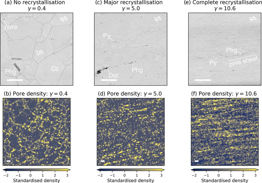
406                     J. Gilgannon et al.: Experimental evidence that viscous shear zones generate periodic pore sheets

Thermodynamic model (cf. Hobbs et al., 2011) known as the           Table 1. Sample porosity.
dynamic granular fluid pump (Fusseis et al., 2009). While
much of this paradigm remains to be tested, the notion that                          Sample     γmax   Porosity (%)
mylonites generate self-sustaining and dynamic pathways for                          PO344       0.4           0.29
mass transport is radical and consequential for the interpre-                        PO422       5.0           0.20
tation of how deep shear zones behave during deformation.                            PO265      10.6           1.15
   The dynamic permeability is proposed to be created and
sustained through the opening and closure of syn-kinematic
pores, called creep cavities, by viscous grain boundary slid-
                                                                    temperature (T = 1000 K, Th = 0.6) with confining pressure
ing during creep (e.g. Herwegh and Jenni, 2001; Dimanov
                                                                    (p = 300 MPa) at constant twist rates. Samples were de-
et al., 2007; Fusseis et al., 2009). In recent years the paradigm
                                                                    formed to large shear strains and during this deformation
has gained traction with many more contributions interpret-
                                                                    recorded the dynamic transformation of undeformed, homo-
ing the presence of, or appealing to, creep cavities in nat-
                                                                    geneous, coarse-grained marbles into fine-grained ultramy-
ural samples (e.g. Gilgannon et al., 2017; Précigout et al.,
                                                                    lonites. The experiments demonstrated that microstructural
2017; Lopez-Sanchez and Llana-Fúnez, 2018; Giuntoli et al.,
                                                                    change by dynamic recrystallisation was concurrent with me-
2020). The most notable claims involving creep cavities are
                                                                    chanical weakening and the development of a strong crystal-
that in polymineralic viscous shear zones their formation es-
                                                                    lographic preferred orientation. More recently, it was shown
tablishes an advective mass transport pump (Fusseis et al.,
                                                                    that these experiments contain creep cavities and that the
2009; Menegon et al., 2015; Précigout et al., 2019), they
                                                                    pores emerged with, and because of, grain-size reduction by
aid melt migration (Závada et al., 2007; Spiess et al., 2012)
                                                                    sub-grain rotation recrystallisation (Gilgannon et al., 2020).
and they have even been speculated to nucleate earthquakes
                                                                    In this contribution we expand on these observations and
(Shigematsu et al., 2004; Dimanov et al., 2007; Rybacki
                                                                    present new results that quantify and contextualise the de-
et al., 2008; Verberne et al., 2017; Chen et al., 2020). How-
                                                                    velopment of porosity inside of an evolving viscous shear
ever, much of the most convincing supporting evidence cur-
                                                                    zone.
rently available is limited to deformation experiments on fab-
                                                                       Please refer to the Appendix for details of the methods
ricated geomaterials and is generally restricted to grain-scale
                                                                    used in the following results.
observations. Hence, it has been difficult to evaluate if this
phenomenon is extensive and relevant at the material scale          2.1   Porosity evolution with mylonitisation
for natural samples and, moreover, if it is applicable to natu-
ral deformations in deep shear zones.                               At very low shear strains, and before any dynamic recrys-
   In this contribution we provide unambiguous experimen-           tallisation, pores decorate grain boundaries and appear as
tal evidence in a natural starting material that supports, and      trails through large grains (d ≈ 200 µm, Fig. 1a). These pores
extends, the paradigm concerning the role of creep cavities         are likely fluid inclusions trapped in and around the orig-
in shear zones. We present quantitative results showing that        inal grains (Covey-crump, 1997) (the pore density map in
creep cavities are generated in periodic sheets making them         Fig. 1b reflects this by highlighting the outlines of the ini-
a spatially significant feature of viscous deformation. Our         tial grain size). In the experiment run to a shear strain of
analyses are intentionally made over large areas of the exper-      5, which is in the midst of significant microstructural ad-
imentally deformed samples in order to contextualise and un-        justment, the porosity has a clearly different character. The
derstand the role of creep cavities at a scale more comparable      pores appear at the triple junctions of small recrystallised
to those where macroscopic material descriptions are unusu-         grains (d ≈ 10 µm) and in some cases are filled with new
ally made. We argue that our results warrant a reappraisal of       precipitates (Fig. 1c). The pore density map of this experi-
the community’s perception of how viscous deformation pro-          ment highlights that pores appear in clusters and that these
ceeds with time in rocks and suggest that the general model         clusters repeat across a large area with a systematic orienta-
for viscous shear zones should be updated to include creep          tion (Fig. 1d). Once the microstructure is fully recrystallised
cavitation. A key consequence of this would be that the en-         (γ = 10.6) and has reached a microstructural steady state, the
ergetics of the deforming system become the keystone of our         porosity forms elongated sheets (Fig. 1e). The density map of
perspective rather than the mechanics.                              this experiment reveals that this porosity has become more
                                                                    spatially extensive and also shows a systematic orientation
                                                                    (Fig. 1f). These pore sheets contain new precipitates of mica,
2   New results from classical experiments                          magnesium calcite and pyrite, implying that the sheets are
                                                                    permeable and act as mass transfer pathways (Fig. 2). When
To make this argument, we have revisited the microstruc-            quantified, it appears that the porosity values before and after
tures of a set of classical shear zone formation experi-            dynamic recrystallisation are similar, but as strain increases
ments performed on Carrara marble (Barnhoorn et al., 2004).         the porosity increases by an order of magnitude (Table 1).
The torsion experiments were run at a high homologous

Solid Earth, 12, 405–420, 2021                                                           https://doi.org/10.5194/se-12-405-2021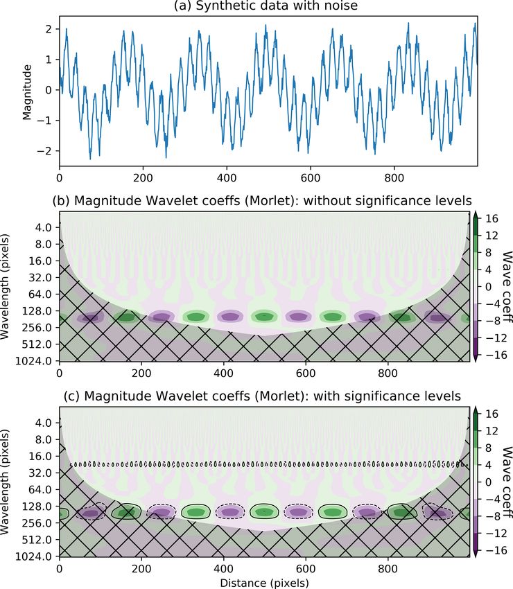
J. Gilgannon et al.: Experimental evidence that viscous shear zones generate periodic pore sheets                                        407

Figure 1. Microstructure and pore density in samples with increasing strain. The samples document the production of a mylonite through
dynamic recrystallisation. Panels (a), (c) and (e) are backscatter electron images while (b), (d) and (f) are pore density maps. In all images
the white scale bar is 100 µm. The pointed ends of the colour bars refer to the fact that some data values are larger than the max and min of
the colour map (Py – pyrite, Dol – dolomite, Phg – phengite, Cc – calcite, gb – grain boundary).

Figure 2. A more detailed view of the pore sheet labelled in Fig. 1e. Please find supporting spectra from energy dispersive spectroscopy
(EDS) in the Appendix for the small precipitates (Py – pyrite, Phg – phengite, Mg-Cc – magnesium calcite).

2.2   2D continuous wavelet analysis of pore sheets                      testing used in climate sciences (Torrence and Compo, 1998)
                                                                         to 2D to filter for noise in the data. Furthermore, by imple-
We quantify the spatial extent and character of these perme-             menting a 2D (pseudo) cone of influence we exclude bound-
able pore sheets with 2D continuous wavelet analysis. In par-            ary effects of the analysis at large wavelengths. For details
ticular, we use the fully anisotropic 2D Morlet wavelet (Neu-            of the wavelet analysis see the Methods section. Fundamen-
pauer and Powell, 2005) to identify features in the pore den-            tally, wavelet analysis can be thought of as a filter that high-
sity maps and expand a 1D scheme of feature-significance                 lights where the analysed data interacts with the wavelet most

https://doi.org/10.5194/se-12-405-2021                                                                   Solid Earth, 12, 405–420, 2021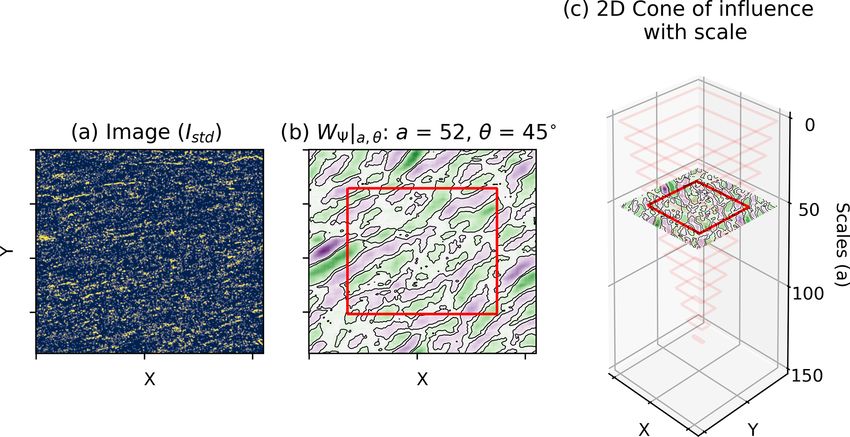
408 J. Gilgannon et al.: Experimental evidence that viscous shear zones generate periodic pore sheets
strongly. By varying the size and orientation (λ and θ in et al., 2006), and Ar that has likely diffused into the sample
Fig. 3a) of the Morlet wavelet, one can isolate significant fea- from the confining medium. While it is unclear what the ex-
tures in the data and gain quantitative information about them act composition of the fluid was, the presence of many newly
including orientation, dimension and any spatial frequency. precipitated minerals in pores, and across pore clusters, is
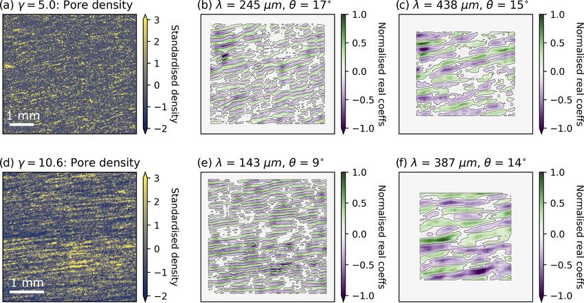
Wavelet analysis reveals that, in both the partly and fully evidence that mass was mobile and redistributed during the
recrystallised samples, porosity is highly ordered with a deformation. Thus if extrapolated to a natural deformation
strong periodicity and anisotropy. Both samples show two where the chemical system may be more open, mass trans-
dominant modes of porosity distribution (Fig. 3b and c). port through this porous network could lead to mass gain or
While the sample is only partly recrystallised, porosity is loss in the mylonite rather than just redistribution. Addition-
preferentially oriented at 17 and 15◦ (measured antithetically ally, our results validate the prediction of pore sheets in the
in relation to the shear plane, see Fig. 3a) with wavelengths of dynamic granular fluid pump model (Fusseis et al., 2009) and
∼ 240 and ∼ 440 µm, respectively (Figs. 3b and 4a–c). This extend it to show that pore sheets can develop spontaneously
is both contrasted and complemented by the modes found in homogenous rocks, with a periodic and oriented charac-
in the fully recrystallised experiment, where the anisotropy ter. Curiously, our results also seem to suggest that porous
is oriented at 9 and 14◦ with wavelengths of ∼ 140 and domains develop within zones of stable orientation and, pos-
∼ 390 µm, respectively (Figs. 3c and 4d–f). Interestingly the sibly, wavelength (approx. 15◦ from the shear zone bound-
longer wavelength porosity features in both samples share ary with a wavelength of 400 µm). This is consequential be-
similar orientations and spacing (11◦ , 150 µm). As wavelet cause it implies that the emergence of porous sheets is de-
analysis does not require that features be periodic to be iden- termined by some bulk material characteristic (for example,
tified, the periodicity is a result and not an artefact of the like the elastic moduli) and not by the positions of any ini-
analysis. tial heterogeneities hosted within the starting material (akin
to grain-size variations). This speculation about the role of a
bulk material characteristic controlling the location of pore
3 Discussion sheet formation is possibly supported by other experimen-
tal observations that the regular spacing of creep fractures
These results provide an unambiguous foundation for dis- from the coalescence of pore sheets changed with temper-
cussing the community’s perception of how viscous defor- ature (see Fig. 16 in Dimanov et al., 2007). What exactly
mation proceeds with time and more generally the role of governs the appearance and location of these apparently sta-
viscous deformation in the conceptual shear zone model. We bly oriented and spaced microstructural adjustments is a clear
claim this because our results show that a mylonitic shear candidate for important future research as it hints at a chal-
zone deforming viscously can spontaneously develop highly lenge to the widely cited role of material inhomogeneity in
anisotropic and periodic porous domains. This is not some- determining the location of deformationally induced trans-
thing that is expected within the prevailing paradigm for the formations and fluid pathways often cited in geological stud-
deformation of rocks at high temperatures and pressures. For ies (e.g. Goncalves et al., 2016; Fossen and Cavalcante, 2017;
this reason it is important for us to reconsider the role of Giuntoli et al., 2020).
mylonites during geochemical, geophysical and hydrological
processes in the lithosphere. 3.2 Does a porous anisotropy affect the mechanics of a
mylonite?
3.1 How mylonites could focus mass transport
Two questions naturally arise from our results: (1) how could
Firstly, we suggest that the presence of periodic, porous the presence of periodic porous sheets affect the mechanical
sheets in natural shear zones would act to focus fluid dur- behaviour of mylonites in the deep lithosphere? and (2) why
ing active deformation. Geochemical studies have proposed did the emergence of a spatially extensive and anisotropic
that the enrichment or depletion of elements in purely vis- porosity not affect the viscous mechanical state recorded in
cous shear zones must reflect syn-deformational fluid mi- the original experiments of Barnhoorn et al. (2004)? Answer-
gration (e.g. Carter and Dworkin, 1990; Selverstone et al., ing these questions is not trivial, but there is some ground to
1991). Our results provide an experimental insight into as- be gained by considering the broader Generalised Thermody-
pects of the syn-kinematic pore network that likely facili- namic literature behind the paradigm concerning creep cav-
tates this fluid transport in natural mylonites. The fluid phase ities and contrasting our results to other experiments where
in our experiments is not constrained but likely some mix creep cavities have been observed to have a mechanical im-
of CO2 , H2 O and Ar. The mixture is expected to be de- pact.
rived from the initial fluid inclusions (of unknown compo-
sitions) in the starting material; from decarbonation of the
dolomite present (cf. Delle Piane et al., 2008); the break-
down of some, but not all, phengite minerals (cf. Mariani
Solid Earth, 12, 405–420, 2021 https://doi.org/10.5194/se-12-405-2021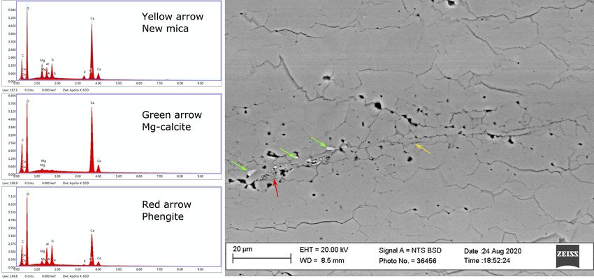
J. Gilgannon et al.: Experimental evidence that viscous shear zones generate periodic pore sheets                                            409

Figure 3. Wavelet analysis of partly (γ = 5.0) and fully (γ = 10.6) recrystallised samples. Panel (a) shows a generic 2D Morlet wavelet. The
wavelet analysis is conducted by considering the wavelet’s interaction with the porosity density maps at each spatial position. This is repeated
for different orientations (θ ) and wavelengths (λ). Panels (b) and (c) visualise the wavelet analysis results for the two samples. Peaks in η
represent the largest interaction with the wavelet (see Sect. A7 for details). Peaks are identified by local extremes in η and marked with red
crosses. We note that two local extremes are not discussed in the text. This is because one was very close to the sensible limit of the analysis
(θ = −12◦ , λ = 530 µm) defined in Appendix A6 and the other did not correlate with any microstructural features (θ = −84◦ , λ = 173 µm).

Figure 4. Visualisation of the results of the wavelet convolution with the pore density maps. The anisotropy identified by the dominant peaks
in Fig. 3 are shown for the partly (a–c) and fully (d–f) recrystallised samples. For each convolution at each wavelength analysed, areas are
defined where edge effects may occur. Data in these areas have been removed, which results in the white areas in the edge of (b) and (c) and
(e) and (f) (see Sect. A6 for details). As before, the pointed ends of the colour bars refer to the fact that some data values are larger than the
max and min of the colour map.

https://doi.org/10.5194/se-12-405-2021                                                                      Solid Earth, 12, 405–420, 2021
410                     J. Gilgannon et al.: Experimental evidence that viscous shear zones generate periodic pore sheets

3.2.1   What effect are creep cavities expected to have in         els (see Fig. 5 in Shawki, 1994). Thus, from a Generalised
        a Generalised Thermodynamic model?                         Thermodynamic perspective, the boundary conditions of our
                                                                   experiments may, in part, explain why we do not see an obvi-
In the dynamic granular fluid pump model, creep cavities are       ous mechanical effect of the porosity with ongoing straining.
predicted to emerge as one of several dissipative processes        Once the steady state microstructure is attained, the sample is
that act to bring the reacting and deforming rock mass into        in a thermodynamic stationary state for the imposed bound-
a thermodynamic stationary state (Fusseis et al., 2009). That      ary velocity that favours a distributed deformation.
is to say that the chief concern of the model is that of the          A constant force boundary condition (also known as
energetics of the system with a focus on the rate of entropy       a constant thermodynamic force boundary condition; cf.
production. Theoretically this means no process is a priori        Regenauer-Lieb et al., 2014; Veveakis and Regenauer-Lieb,
excluded from activating and the most efficient combination        2015) is predicted to produce instability and localisation
of processes that use and store energy act in congress to pro-     in rock deformation at high homologous temperatures (e.g.
duce a thermodynamic stationary state (Fusseis et al., 2009;       Fressengeas and Molinari, 1987; Paterson, 2007). It is often
Regenauer-Lieb et al., 2009, 2015); the system is neither ac-      assumed that plate boundaries in nature will be under such a
celerating or decelerating in a dissipative sense but is in some   boundary condition (cf. Alevizos et al., 2014) and in this in-
kind of steady state. Therefore, in this model, many factors       stance the presence of anisotropic domains of porosity may
play a role in determining whether or not creep cavities will      have a different impact than in our experiments. For example,
affect the mechanical state of the deforming body.                 in experiments not dissimilar in geometry to our own, run on
   One of the factors that may be pertinent to our experiments     olivine, it was found that localisation did indeed occur at con-
is the boundary conditions for deformation. It is known from       stant force conditions and not for constant velocity (Hansen
various types of modelling that different boundary condi-          et al., 2012). At a constant force this localisation was ex-
tions, i.e. constant force vs. constant velocity, can promote      pressed both in the microstructural adjustments (with the de-
or inhibit material instability and localisation (e.g. Fressen-    velopment of an oriented foliation and domains of varying
geas and Molinari, 1987; Cherukuri and Shawki, 1995; Pater-        grain size) and in the mechanical behaviour of the olivine
son, 2007). In the case of constant velocity boundary condi-       aggregates (noted by a continual weakening of the samples
tions, like those applied in our torsion experiments, localisa-    beyond a shear strain of 0.5). If we speculate on how our ex-
tion is not expected to occur (e.g. Fressengeas and Molinari,      periments may have proceeded under constant force bound-
1987; Paterson, 2007). Indeed, from a Generalised Thermo-          ary conditions, it could be that porous domains emerge with
dynamic perspective, when the boundary conditions are set          some similar modes of periodicity to those observed under
to a constant thermodynamic flux, i.e. a constant velocity         a constant velocity, but in this case they might provide the
(like the experiments we revisit; cf. Regenauer-Lieb et al.,       sites for some kind of instability. For example, in our hypo-
2014), the dissipative conditions are fixed and the material is    thetical case, pore sheets may aid in establishing features like
forced to meet them through the activation of as many dissi-       the high frequency foliation and lower frequency domains of
pative micro-mechanisms at as many positions in the rock as        grain-size variation observed by Hansen et al. (2012) (e.g.
necessary (cf. Veveakis and Regenauer-Lieb, 2015; Guével           Figs. 5c and d and 9a in Hansen et al., 2012). Of course,
et al., 2019). Conducting a deformation experiment in this         our speculation is only that, and this line of argument re-
fashion means that the onset of a localising instability can       quires new experimental testing that is beyond the scope of
be missed because the rock is not allowed to incrementally         our revisiting of the classical experiments of Barnhoorn et al.
adjust to an incrementally applied energy input (e.g. Peters       (2004). What it does highlight is that viscous deformation in
et al., 2016). This does not prohibit the possibility of local     mylonites requires more research to understand exactly when
microstructural differences developing, but it does mean that      and where a periodic occurrence of creep cavities could have
at the scale of the material a distributed deformation can         a mechanical impact.
remain favourable despite a heterogeneous microstructure.
This observation of a stable but heterogeneous microstruc-         3.2.2   A comparison to other experiments that
ture suggests that the size of the heterogeneities produced                developed domains of creep cavities
are not sufficiently large to impose further localisation. In
the work of Shawki (1994) it was shown that thermal pertur-        In this context, there are four other experimental works in
bations below a critical wavelength would not impose local-        which creep cavities were documented to develop that are
isation during constant velocity boundary conditions. If the       worth comparing to our results. All of these experiments
variation in creep cavity domains reflect different amounts        were run in torsion with constant twist rates (constant ther-
of work being dissipated locally, and hence heat being pro-        modynamic flux boundary conditions) at high confining pres-
duced, then one can see that the shorter wavelength porous         sures and homologous temperatures on synthetic dolomite
domains, which reflects the size of actual pore sheets (Fig. 2),   (Delle Piane et al., 2008), synthetic gabbro (Dimanov et al.,
are below the size of the thermal heterogeneities that were        2007) and synthetic anorthite aggregates (Rybacki et al.,
found to impose localisation in the constant velocity mod-         2008, 2010). All experiments developed creep cavities in

Solid Earth, 12, 405–420, 2021                                                          https://doi.org/10.5194/se-12-405-2021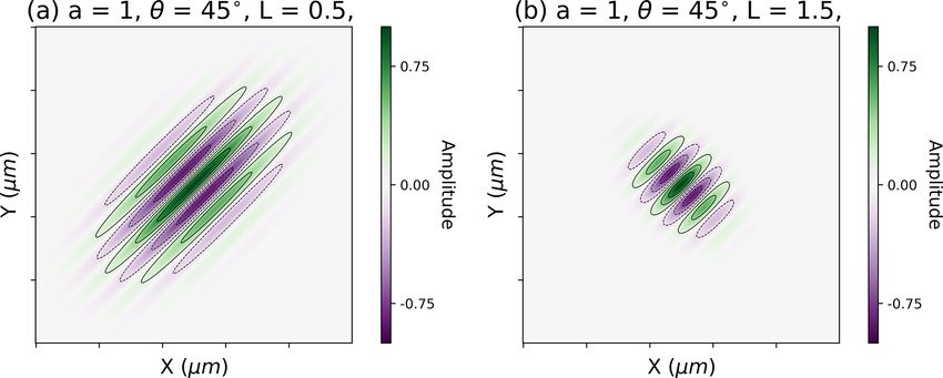
J. Gilgannon et al.: Experimental evidence that viscous shear zones generate periodic pore sheets                               411

oriented and spaced domains during linear viscous flow.             5 (e.g. Dimanov et al., 2007; Rybacki et al., 2008, 2010) with
In the gabbroic and some of the anorthitic samples, these           others flowing up to a shear strain of 50 with no fractures
porous domains became sites for the generation of instabili-        developing (Barnhoorn et al., 2004). This observation also
ties known as creep fractures (Dimanov et al., 2007; Rybacki        seems to highlight a limitation to the use of empirical rela-
et al., 2008, 2010). When one compares the four experimen-          tionships that link strain or time to failure by creep fracture
tal sets to our samples and to one another, it is clear there are   (e.g. Rybacki et al., 2008). Taken together, we suggest that
many differences and similarities. Firstly, the starting mate-      this potential disconnection between the microstructure and
rials are all compositionally different and have various initial    mechanics of a mylonite places a need for the use of more
mean grain sizes, grain shapes and grain size distributions.        complex physics to describe how a shear zone may deform
Secondly, all four of these experiments use fabricated sam-         with time.
ples in comparison to our natural Carrara marble samples.              This point complements the fact that the dynamic granular
Thirdly, when domains of creep cavities did emerge in the           fluid pump model (Fusseis et al., 2009), which our work tests
four experiments, some produced bands that were broadly             aspects of, requires the consideration of energy, mass and
a mirrored orientation to our results around the shear plane        momentum balance alongside rate equations for irreversible
(see Figs. 14 and 16 in Dimanov et al., 2007, Fig. 1 in Ry-         physical deformation (like plastic or viscous flow laws) and
backi et al., 2008, Fig. 6 in Rybacki et al., 2010 and Fig. 2       both reversible and irreversible chemical processes (Fusseis
in Spiess et al., 2012) with others being similarly oriented to     et al., 2009; Regenauer-Lieb et al., 2009, 2015). These dif-
our results (see Fig. 8a in Delle Piane et al., 2008 and Fig. 5     ferent dissipative processes act at different diffusive length
in Rybacki et al., 2010). Lastly, for the gabbroic and anor-        scales and are predicted to account for the geometry and
thitic experiments these oppositely oriented porous domains         temporal variation of several phenomena that all act syn-
were reported to evolve into fractures while those domains          chronously during a deformation (cf. Regenauer-Lieb et al.,
of a similar orientation to our results did so less or not at       2015). In this perspective, a flow law(s) is necessary but not
all (Dimanov et al., 2007; Rybacki et al., 2008, 2010) and          sufficient to fully describe a deformation, with the balancing
never in the dolomite experiments where linear viscous flow         of the energy equation being of chief importance. Said an-
was maintained (Delle Piane et al., 2008). It is not clear what     other way, many thermally activated rate equations for phys-
critical condition leads some to fracture and others to not. For    ical processes may compete to dissipate energy and collec-
example, is it the local pore density, differences in pore fluid    tively produce a bulk mechanical diffusivity (Veveakis and
pressure or the widths of the porous domains that controls if       Regenauer-Lieb, 2015). While our results cannot speak to all
a fracture develops? While it is hard to draw any categori-         of these claims, they do show that there is some validity to the
cal conclusions from the comparison of these experiments, it        predictions of this newer paradigm, namely the emergence of
is noteworthy that in each experimental case the mechanical         pore sheets. This generally adds weight to older discussions
data recorded a viscous deformation, regardless of whether          about the possible need for a more complex view of defor-
fracture instabilities occurred or not. This point draws atten-     mation in mylonites (Evans, 2005; Mancktelow, 2006; Di-
tion to a conclusion already made in the seminal work of            manov et al., 2007) and suggests further testing is needed of
Dimanov et al. (2007), “[c]learly, the ‘microstructural state’      the Generalised Thermodynamic ideas behind the paradigm
is not obviously representative of the ‘mechanical state’.”. If     concerning creep cavities.
this holds true for mylonites in nature then it opens an am-
biguity over how the deformation of a mylonite will proceed         3.3   Some consequences of incorporating creep cavities
with time: will it fracture, or will it flow?                             into the conceptual shear zone model

3.2.3   Is a flow law enough to describe a mylonite?                There are several enigmatic observations that are not well ac-
                                                                    counted for in the current conceptual model for lithospheric
Our results, and those of the four other experiments described      shear zones. To name a few: there is field evidence of fric-
above, suggest that mylonites of various compositions de-           tional melting in the deep crust (e.g. Hobbs et al., 1986),
velop complicated microstructures that for an unknown set           the intrusion of dykes during upper amphibolite facies condi-
of critical conditions can facilitate a spontaneous mechan-         tions (Weinberg and Regenauer-Lieb, 2010) and the fact that
ical change from flow to fracture. While there are many             some geophysical data suggest that slow earthquake phenom-
ways to incorporate history dependence into flow laws that          ena can occur at depths below the seismogenic zone (Wang
account for some microstructural change (cf. Renner and             and Tréhu, 2016). If the new evidence we present, namely
Evans, 2002; Barnhoorn et al., 2004; Evans, 2005), it does          that mylonites can develop periodic porous domains during
not seem that this kind of rate equation would capture the          a viscous deformation, is incorporated into our conceptual
differences between ours and the four other experiments de-         model for lithospheric shear zones, many new possible expla-
scribed. For example, a flow law that integrated strain (e.g.       nations emerge for otherwise hard to explain observations.
Hansen et al., 2012) would not be able to account for why              In the case of dyke intrusion at high grade conditions, the
some of the five experiments fractured at shear strains below       work of Weinberg and Regenauer-Lieb (2010) in fact already

https://doi.org/10.5194/se-12-405-2021                                                           Solid Earth, 12, 405–420, 2021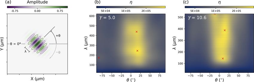
412                    J. Gilgannon et al.: Experimental evidence that viscous shear zones generate periodic pore sheets

invoked creep cavities and their coalescence into creep frac-        Moreover, any instability of pore sheets in natural plate
tures as the responsible mechanism for allowing dyking to         boundaries may factor into explaining how both ambient and
occur. While our results do not show the development of           teleseismically triggered tremors can occur at depths below
creep fractures, they forward the speculative argument of         the seismogenic zone (Wang and Tréhu, 2016). This could
Weinberg and Regenauer-Lieb (2010) that creep cavities will       place sheets of creep cavities alongside brittle fracturing and
occur during ductile shearing in rocks and could be inter-        non-isochoric chemical reactions as the potential nuclei of
preted to add weight to the discussion of Spiess et al. (2012)    slow earthquake phenomena. As the emergence of creep
about the grain-scale role of creep cavities in promoting melt    cavities was linked to dynamic recrystallisation (Gilgannon
segregation and flow. When this is considered alongside the       et al., 2020), a process expected throughout the lithosphere,
body of seminal experimental work on partially molten rocks       the porous anisotropy presented here would allow slow earth-
(e.g. Kohlstedt and Holtzman, 2009), it becomes clear that        quake phenomena to occur across a range of metamorphic
tests need to be devised to distinguish between the different     conditions and mineralogical compositions (Peacock, 2009).
theories of melt segregation and migration (e.g. compaction
length vs. sheets of creep cavities).
   Additionally, recent experiments on calcite gouges made        4   Conclusions
observations of creep cavities and argued that their forma-
                                                                  In summary, the current paradigm of viscosity that is bor-
tion allowed the gouge to transition from flow to friction
                                                                  rowed from fluids is not a completely adequate analogy for
(Chen et al., 2020). While these were lower temperature ex-
                                                                  solid geomaterials. We claim this because we observe that
periments than our own, they reinforce the notion that rocks
                                                                  during the formation of a mylonite, which was recorded to
could spontaneously transition from a viscous rheology to
                                                                  possess viscous mechanical properties, a heterogeneous mi-
another mechanical state. This is relevant for observations of
                                                                  crostructure of periodic porous domains emerged. The cur-
deep seated frictional melting where the presence of a porous
                                                                  rent paradigm of viscosity in rocks does not expect this to
anisotropy in mylonites may facilitate changes to some kind
                                                                  occur and we have discussed how this observation of pore
of granular or frictional mechanical mode that is otherwise
                                                                  sheet formation during viscous deformation is seen in at least
unexpected. This would complement earlier work that sug-
                                                                  four other experiments of differing compositions. The porous
gested that the mechanical behaviour of mylonites may be
                                                                  anisotropy we observe likely has a role to play in both the
more pressure dependent than generally assumed (Manck-
                                                                  transport of mass and the mechanics of the lithosphere. On
telow, 2006) and the emergence of creep cavities with high
                                                                  this basis, we advocate for an update to the current concept
strains would facilitate this.
                                                                  of viscosity at high temperatures and pressures in rocks to in-
   In the case of quartz and calcite-dominated crustal-scale
                                                                  clude the periodic porous anisotropy we have presented. Our
shear zones there often exists a peculiar relationship between
                                                                  discussion has explored some of the possible consequences
viscous strain localisation in ultramylonites, fracturing and
                                                                  of changing our paradigm and, moving forward, these specu-
precipitation of syn-kinematic veins/–fluid flux within these
                                                                  lations should be further tested. As the viscosity of solids is a
ultramylonites (e.g. Badertscher and Burkhard, 2000; Her-
                                                                  cornerstone of geoscience, our results have farther reaching
wegh and Kunze, 2002; Herwegh et al., 2005; Haertel et al.,
                                                                  implications than the conceptual shear zone model and may
2013; Poulet et al., 2014; Tannock et al., 2020) . In the
                                                                  even be relevant for other scenarios where solid state defor-
wake of our results, it is tempting to propose that this syn-
                                                                  mation is modelled with viscous rheologies like glacial flow
kinematic veining may be related to an interplay of fluid
                                                                  (e.g. Egholm et al., 2011) and tectonics on exoplanets (e.g.
transport and the instability of the anisotropic porous do-
                                                                  Noack and Breuer, 2014).
mains. This is especially so for cases like the deeper portions
of the basal shear zones of the nappes of the Helvetic Alps,
where veining is observed to broadly increase with proxim-
ity to ultramylonitic shear zones (cf. Herwegh and Kunze,
2002) that are expected to be purely viscous in our current
mechanical paradigm of the crust.

Solid Earth, 12, 405–420, 2021                                                         https://doi.org/10.5194/se-12-405-2021
J. Gilgannon et al.: Experimental evidence that viscous shear zones generate periodic pore sheets 413
Appendix A: Methods Table A1. Experimental samples revisited.
The results of the main article come from the investigation of Sample γ̇ γmax Amount of recrystallisation
three experimental samples (see Table A1). Each sample was
PO344 3 × 10⁻⁴ 0.4 none
imaged using scanning electron microscopy, segmented and
PO422 3 × 10⁻⁴ 5.0 majora
analysed. In the following, the data acquisition, processing
PO265 2 × 10⁻³ 10.6 completeb
and analysis used is outlined. For a description of the starting
material or the original experimental procedure please refer a 65 %–90 % as classified by Barnhoorn et al. (2004). b 90 %–100 % as
to Barnhoorn et al. (2004) and Gilgannon et al. (2020). classified by Barnhoorn et al. (2004)
A1 Acquisition of large backscatter electron mosaics Table A2. Dimensions and resolutions of mosaics.
Three large BSE maps were acquired on a Zeiss Evo 50 SEM Sample γmax Pixel dimensions Scale (px : µm)
with a QBSD semiconductor electron detector (acceleration
voltage = 15 kV; beam current ≈ 500 pA). In each case the PO344 0.4 15 000 × 13 944 1 : 0.36
PO422 5.0 8745 × 7392 1 : 0.55
maps were stitched together by the Zeiss software Multiscan.
PO265 10.6 21 127 × 20 494 1 : 0.16
The pixel dimensions and scales are listed in Table A2.
A2 Segmentation for porosity
here was to retain as much data as possible in the visualisa-
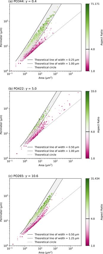
We used the segmentation, labelling and filtering work flow tion. In this way we visualised local neighbourhoods and pro-
described in Gilgannon et al. (2020) for open pore space. In duced an image for further analysis that had not been overly
this work flow grain boundaries must be filtered for by using smoothed. It was these density maps that we then quantita-
each labelled feature’s aspect ratio. Specifically, the data are tively analysed with 2D continuous wavelet analysis.
filtered to remove features with aspect ratios greater than 4.
Figure A1 shows all features initially labelled as porosity by A4 2D continuous wavelet analysis
the segmentation process in each sample. These are plotted
for their area and perimeter, while colour coded for aspect Wavelets are highly localised waveforms that can be used to
ratio. In each data set there are two trends: analyse signals with rising and falling intensity. Our images
are such signals. Simply put, wavelets can be used to reveal
1. features with aspect ratios > 4 that show area–perimeter
the location (in space or time) and the frequency at which the
relationships for lines of widths between 0.25–1.25 µm
most significant parts of a signal can be found. Continuous
2. features with aspect ratios < 4 that do not show, area– wavelet analysis is the particular wavelet-based method that
perimeter relationships of a line. we employ in this contribution.
To identify features at different frequencies, the wavelet is
Based on these criteria, only features with aspect ratios of stretched over what are known as different scales (a). The
< 4 are considered as pores. The centres of mass of features scales relate to the central frequency of the wavelet, which in
meeting this criteria were then extracted and used in the ker- turn can be related to the wavelength (λ):
nel point density analysis.
4π a
A3 Kernel density estimator maps λ= q , (A1)
k0 + k02 + 4
At the first instance, one of the major difficulties in under-
standing the relationship of micrometre-scale features across where k0 is the wavenumber.
millimetres is simply visualising the problem. We utilised the In the broadest sense, a wavelet can be seen as a filter
kernel density (KDE) for point features function in ESRI’s that finds peaks in an image. To do this it is shifted around
ArcGIS v10.1 software to overcome this issue. This has the the spatial domain (x) of an image, by way of the shift pa-
effect of converting point data, which only tell us something rameter (b), and this is repeated at different scales to find
about individual pores, to a map that considers the distribu- peaks. In this way features of different sizes can be located
tion of pores and, in part, their relation in space. in space and in scale: short wavelengths highlight small fea-
We manually set the output cell size and search radius to 1 tures and long wavelengths larger ones. In this contribution,
and 20 µm, respectively. The kernel smoothing factor was au- we utilise the fully anisotropic Morlet wavelet (Neupauer and
tomatically calculated with reference to the population size Powell, 2005) because it also allows features of varying ori-
and the extent of analysis and contoured based on a 1/4σ entation to be identified. The wavelet is considered to be fully
kernel. We specifically did not use the default search radius anisotropic because it produces in-phase elongation along the
(calculated with Silverman’s Rule of Thumb). Our intention wave vector, such that the wavelet can be rotated and main-
https://doi.org/10.5194/se-12-405-2021 Solid Earth, 12, 405–420, 2021414 J. Gilgannon et al.: Experimental evidence that viscous shear zones generate periodic pore sheets
Figure A2. Examples of how a wavelet changes with the anisotropy
ratio (L).
This rotation matrix rotates the entire wavelet by θ , which
is defined as positive in a counter-clockwise direction with
respect to the positive x axis (see Fig. 3 of the main article):
L 0
A= , (A5)
0 1
where the ratio of anisotropy (L) is defined as the ratio of
the length of the wavelet perpendicular to θ over the length
parallel to θ . In this way, values of L < 1 represent extreme
anisotropy parallel to the angle of the wavelet.
We chose to use an anisotropy ratio of L = 1.5 (see
Fig. A2). This was done because the input images are kernel
density maps and the estimator used is circular. We wanted
our wavelet to utilise its inherent anisotropy and angular se-
lectivity to identify extended concentrations of the estimator
that would appear as elliptical clusters of circles. We did not
use an L < 1 as these wavelets anisotropies are too far from
the shapes expected from the features we investigated (Tor-
rence and Compo, 1998). If, for example, we had been inves-
tigating linear features like fractures we would have used a
more anisotropic wavelet shape (for example, L = 0.5).
To ensure that the total energy of the analysing wavelet is
independent of the scale of analysis the relationship between
the wavelet (Eq. A2) and the mother wavelet is
√
Figure A1. Filtering criteria for grain boundaries and pores. L x −b
9 a,b (x, θ, L) = 9 , θ, L . (A6)
a a
tain its anisotropy. The wavelet takes the form: To be clear, we refer above to energy in the generalised
T ACx)
sense of signal processing.
9(x, θ, L) = eik 0 ·Cx e−1/2(Cx·A , (A2) Our input images for wavelet analysis are 32-bit kernel
density maps for the centres of mass of open pores. Each
where θ , L, k 0 , C and A are the angle for the rotation ma-
density map can be considered as an intensity function (I (x))
trix, ratio of anisotropy, wave vector, rotation matrix and
whose magnitude limits are that of the KDE density calcula-
anisotropy matrix, respectively. The non-scalar terms are
tion. We standardise each input image such that
given by
I −µ
k 0 = (0, k0 ), k0 > 5.5. (A3) I std (x) = , (A7)
σ
In this study we use k0 = 6.0. where µ and σ are the image’s mean and standard devia-
tion. This is because the best results of wavelet analysis are
cos θ − sin θ achieved on a zero-mean random field (Neupauer and Pow-
C= (A4)
sin θ cos θ ell, 2005).
Solid Earth, 12, 405–420, 2021 https://doi.org/10.5194/se-12-405-2021J. Gilgannon et al.: Experimental evidence that viscous shear zones generate periodic pore sheets 415
It is on this new standardised image that we perform
the wavelet transformation. The wavelet transformation of
I std (x) is a convolution with the analysing wavelet:
√ Z∞
L x −b
W 9 f (b, a, θ, L) = f (x)9̄ , θ, L dx
a a
−∞
(A8)
√
L b
= f (b)∗9̄ − , θ, L .
a a
Here, ∗ is the convolution and the overbar denotes the
complex conjugate. The convolution is evaluated by tak-
ing the inverse fast Fourier transform of the products of the
Fourier transforms of f (b) and 9̄(−b/a, θ, L). This wavelet
and the convolution follow those outlined in Neupauer and
Powell (2005).
A5 Defining significance
As outlined above, wavelet analysis will highlight regions of
an image where the wavelet and the image interact strongly.
This interaction alone is not enough to say that what the
wavelet highlighted is relevant when compared to any ex-
pected noise in the image. Therefore, it is important to know Figure A3. Example of why a significance test is needed. Panel (a)
if the areas highlighted by the wavelet are significant. To de- is a 1D synthetic, noisy signal made of two waves of different wave-
fine what is significant in the analysis we adopt the method lengths. Panels (b) and (c) present the 1D wavelet transformation of
outlined in Torrence and Compo (1998). (a) with a 1D Morlet wavelet. In (b), the result is only visualised,
while in (c) the significance test is also visualised. In both, the
The general assumption of the null hypothesis is that the
hatched area contains edge effects and is delimited by a 1D cone of
image analysed has some mean power spectrum (Pk , see
influence. The contouring in (c) shows domains that are within the
Eq. 16 in Torrence and Compo, 1998) related to a back- 95 % confidence level of not being white noise. The contours high-
ground geophysical process(es). If the wavelet power spec- light values that are both positively and negatively larger than the
trum is found to be significantly above this background spec- white noise model. The takeaway message is that the significance
trum then the feature is a real anomaly and not a result of the test is needed to accurately identify regions of “real anomaly”.
assumed background process(es).
To test the null hypotheses, the local wavelet power spec-
trum at each scale (following Eq. 18 in Torrence and Compo, assumes a uniform power across frequencies. We chose this
1998) must be considered: because we wish to identify when porosity density is non-
|Wb (a)2 | 1 random and, based on our knowledge of the active processes,
2
H⇒ Pk χ22 , (A9) we consider that any noise will be uniform across the scales
σ 2
of analysis. We make this assumption about the background
where |Wb (a)2 | is the local power, σ 2 is the variance, H⇒ spectra for the following reasons.
indicates “is distributed as” and χ22 represents a chi-square The experiments we revisit are non-localising at the sam-
distribution with two degrees of freedom. Using the relation ple scale and are considered as the exemplar of a sub-solidus,
in Eq. (A9) one can find how significantly the local wavelet homogenous, viscous deformation. The prevailing assump-
power deviates from the background spectrum. To do this, tion for such a sample being deformed is that the microstruc-
the mean background spectrum, Pk (where k is the Fourier tural change will first occur where locally favourable condi-
frequency), is multiplied by the 95th percentile value of χ22 tions allow. For example, some poorly oriented grains may
to give a 95 % confidence level. As the local wavelet power is develop more deformation induced defects and be prone to
distributed equivalently, this confidence level can be used to recrystallise earlier than other grains. The general distribu-
contour the global wavelet power (|W 9 2 |). The result allows tion of grain orientations is determined by the starting ma-
the identification of data that has a 95 % chance of not being terial’s texture, which in the case of Carrara marble is ran-
a random peak from the background spectrum (see Fig. A3). dom (Pieri et al., 2001). Therefore, as there is not any initial
In this contribution we adopted a white noise model as anisotropy in grain orientations, it is expected that porosity
our background spectra. White noise is a random signal that will form randomly in space at favourable sites in the mi-
https://doi.org/10.5194/se-12-405-2021 Solid Earth, 12, 405–420, 2021416 J. Gilgannon et al.: Experimental evidence that viscous shear zones generate periodic pore sheets
crostructure. Any deviation from this expectation is of inter- In this way, our COI does not account for the wavelet’s
est to us. For these reasons, we use a white noise model as shape and anisotropy. While this means our COI is not the
our background spectra and it forms the reference for testing correct mathematical solution for defining where edge effects
where the porosity density is non-random. end for this 2D wavelet, it is a best first attempt at defining
As stated in the main text, it was shown for our experi- a limit to the analysis. We then delete data that lie within the
ments that creep cavities emerged with, and because of, grain COI. Furthermore, we define a sensible limit to the largest
size reduction by sub-grain rotation recrystallisation (Gilgan- relevant scale of analysis by only considering scales that have
non et al., 2020). The white noise null hypothesis used sup- edge-effect-free windows that are greater than 30 % of the
poses that this grain size change and porosity development original image size.
occurred with no preference in space or frequency. By using
this as our null model we can show when the wavelet analysis A7 Visualising wavelet results
produces interactions that are very unlikely to have occurred
randomly and highlights heterogeneity and anisotropy in the Figure 3 of the main article uses the global measure η (Neu-
porosity density maps. pauer et al., 2006) to investigate peaks in the data. Here we
define η as
A6 Defining limits of the analysis Z
η(a, θ, L) = |W 9 2 | db. (A10)
As images have finite length and width, the analysing wavelet
will misinterpret these edges and produce erroneously posi- As we use only one value of anisotropy, η can be visualised
tive results. To avoid this, one may use padding but ultimately to reveal information about peaks in orientation and scale.
the problem will remain (Torrence and Compo, 1998). In- To quantitatively identify peaks in η we use the h_maxima
stead, we have chosen to implement a 2D cone of influence function (where h = 0.03) of the Scikit-image python library
(COI). Starting from the edge of the image, the COI defines (van der Walt et al., 2014).
a zone in which data will likely suffer from edge effects
(see area outside of red contour in Fig. A4b). The zone in- A8 Energy dispersive spectroscopy (EDS) spectra of
creases proportionally with the wavelet scales. We consider small precipitates in the pore sheet
our 2D COI as a pseudo-COI because we simply project two
1D COIs across the 2D surface. We use the e-folding time Point analysis was used to collect spectra with energy disper-
defined by Torrence √ and Compo (1998) for their 1D Morlet sive spectroscopy (EDS) of the small precipitates in the pore
wavelet, which is 2a. For both the y and x axis of the in- sheet presented in Fig. 2 of the main article. These data are
put image we can calculate the appropriate length 1D COI. shown alongside a higher resolution BSE image taken un-
Each of these 1D COIs is calculated for the set of discrete der high vacuum on the same Zeiss Evo 50 SEM described
scales defined for the wavelet transformation. At each scale, above.
the y and x axis COIs are projected to produce a contour that
defines the 2D COI at each scale (see Fig. A4b and c).
Solid Earth, 12, 405–420, 2021 https://doi.org/10.5194/se-12-405-2021J. Gilgannon et al.: Experimental evidence that viscous shear zones generate periodic pore sheets 417 Figure A4. Defining the limits of the analysis across scales. For some image (a), an arbitrary wavelet transformation is visualised at an arbitrary scale and angle (b). Here, the black contours enclose data that are within the 95 % confidence level. Overlaying this is a red contour that delimits the zone of possible edge effects of the analysis. At this scale, this is a slice of the cone of influence (COI). Panel (c) visualises the COI across scales. As the scale, and therefore the wavelength, of the analysing wavelet increases, the zone without edge effects decreases. For the purposes of demonstration, data within the COI have not been removed in this figure. Figure A5. Energy dispersive spectroscopy (EDS) spectra of small precipitates in the pore sheet shown in Fig. 2 of the main article. https://doi.org/10.5194/se-12-405-2021 Solid Earth, 12, 405–420, 2021
418                       J. Gilgannon et al.: Experimental evidence that viscous shear zones generate periodic pore sheets

Code and data availability. Data and code are available from            Carter, K. and Dworkin, S.: Channelized fluid flow
the Bern Open Repository and Information System (BORIS,                   through shear zones during fluid-enhanced dynamic
https://boris.unibe.ch/, last access: 17 February 2021) under             recrystallization,     Northern       Apennines,       Italy,   Ge-
https://doi.org/10.7892/boris.151266 (Gilgannon, 2021).                   ology,       18,      720–723,        https://doi.org/10.1130/0091-
                                                                          7613(1990)0182.3.CO;2, 1990.
                                                                        Chen, J., Verberne, B., and Niemeijer, A.: Flow-to-Friction Transi-
Author contributions. JG, TP, AlB and MH designed the study. JG           tion in Simulated Calcite Gouge: Experiments and Microphysi-
and MW implemented the wavelet method. AuB ran the original               cal Modelling, J. Geophys. Res.-Sol. Ea., 125, e2020JB019970,
experiments. All authors were involved in the interpretation of the       https://doi.org/10.1029/2020JB019970, 2020.
results and the writing of the final manuscript.                        Cherukuri, H. and Shawki, T.: An energy-based localiza-
                                                                          tion theory: I. Basic framework, Int. J. Plast., 11, 15–40,
                                                                          https://doi.org/10.1016/0749-6419(94)00037-9, 1995.
Competing interests. The authors declare that they have no conflict     Covey-crump, S.: The high temperature static recovery and
of interest.                                                              recrystallization behaviour of cold-worked Carrara marble,
                                                                          J. Struct. Geol., 19, 225–241, https://doi.org/10.1016/S0191-
                                                                          8141(96)00088-0, 1997.
                                                                        Delle Piane, C., Burlini, L., Kunze, K., Brack, P., and Burg,
Acknowledgements. We would like to thank Klaus Regenauer-Lieb
                                                                          J.-P.: Rheology of dolomite: Large strain torsion experi-
for several stimulating discussions about the role of creep cavities
                                                                          ments and natural examples, J. Struct. Geol., 30, 767–776,
and rock rheology in general. We thank Federico Rossetti for his
                                                                          https://doi.org/10.1016/j.jsg.2008.02.018, 2008.
role as editor alongside Alberto Ceccato and Lars Hansen for their
                                                                        Dimanov, A., Rybacki, E., Wirth, R., and Dresen, G.: Creep and
constructive reviews that helped improve the final manuscript.
                                                                          strain-dependent microstructures of synthetic anorthite-
                                                                          diopside aggregates, J. Struct. Geol., 29, 1049–1069,
                                                                          https://doi.org/10.1016/j.jsg.2007.02.010, 2007.
Financial support. This research has been supported by                  Edmond, J. and Paterson, M.: Volume changes during the deforma-
the Schweizerischer Nationalfonds zur Förderung der Wis-                  tion of rocks at high pressures, Int. J. Rock Mech. Min. Sci., 9,
senschaftlichen Forschung (grant no. 162340).                             161–182, https://doi.org/10.1016/0148-9062(72)90019-8, 1972.
                                                                        Egholm, D., Knudsen, M., Clark, C., and Lesemann, J.: Modeling
                                                                          the flow of glaciers in steep terrains: The integrated second-order
Review statement. This paper was edited by Federico Rossetti and          shallow ice approximation (iSOSIA), J. Geophys. Res.-Earth,
reviewed by Lars Hansen and Alberto Ceccato.                              116, F02012, https://doi.org/10.1029/2010JF001900, 2011.
                                                                        Evans, B.: Creep constitutive laws for rocks with evolv-
                                                                          ing structure, Geol. Soc. Spec. Publ., 245, 329–346,
                                                                          https://doi.org/10.1144/GSL.SP.2005.245.01.16, 2005.
References                                                              Fossen,      H.     and      Cavalcante,      G.:      Shear    zones
                                                                          – A review, Earth Sci. Rev., 171, 434–455,
Alevizos, S., Poulet, T., and Veveakis, E.: Thermo-poro-mechanics         https://doi.org/10.1016/j.earscirev.2017.05.002, 2017.
  of chemically active creeping faults. 1: Theory and steady            Fressengeas, C. and Molinari, A.: Instability and localization of
  state considerations, J. Geophys. Res.-Sol., 119, 4558–4582,            plastic flow in shear at high strain rates, J. Phys. Chem. Solids,
  https://doi.org/10.1002/2013JB010070, 2014.                             35, 185–211, https://doi.org/10.1016/0022-5096(87)90035-4,
Badertscher, N. and Burkhard, M.: Brittle–ductile deformation in          1987.
  the Glarus thrust Lochseiten (LK) calc-mylonite, Terra Nova,          Fusseis, F., Regenauer-Lieb, K., Liu, J., Hough, R., and
  12, 281–288, https://doi.org/10.1046/j.1365-3121.2000.00310.x,          De Carlo, F.: Creep cavitation can establish a dynamic gran-
  2000.                                                                   ular fluid pump in ductile shear zones, Nature, 459, 974–977,
Barnhoorn, A., Bystricky, M., Burlini, L., and Kunze, K.: The role        https://doi.org/10.1038/nature08051, 2009.
  of recrystallisation on the deformation behaviour of calcite rocks:   Gilgannon, J.: se-2020-137_dataset_and_code, BORIS, available
  large strain torsion experiments on Carrara marble, J. Struct.          at: https://doi.org/10.7892/boris.151266, 2021.
  Geol., 26, 885–903, https://doi.org/10.1016/j.jsg.2003.11.024,        Gilgannon, J., Fusseis, F., Menegon, L., Regenauer-Lieb, K., and
  2004.                                                                   Buckman, J.: Hierarchical creep cavity formation in an ultramy-
Beach, A.: The Interrelations of Fluid Transport, Deformation, Geo-       lonite and implications for phase mixing, Solid Earth, 8, 1193–
  chemistry and Heat Flow in Early Proterozoic Shear Zones in the         1209, https://doi.org/10.5194/se-8-1193-2017, 2017.
  Lewisian Complex, Philos. Trans. Royal Soc. A, 280, 569–604,          Gilgannon, J., Poulet, T., Berger, A., Barnhoorn, A., and Her-
  1976.                                                                   wegh, M.: Dynamic recrystallisation can produce porosity
Beall, A., Fagereng, Å., and Ellis, S.: Fracture and Weakening of         in shear zones, Geophys. Res. Lett., 47, e2019GL086172,
  Jammed Subduction Shear Zones, Leading to the Generation of             https://doi.org/10.1029/2019GL086172, 2020.
  Slow Slip Events, Geochem. Geophy. Geosy., 20, 4869–4884,             Giuntoli, F., Brovarone, A., and Menegon, L.: Feedback be-
  https://doi.org/10.1029/2019GC008481, 2019.                             tween high-pressure genesis of abiotic methane and strain lo-
Bürgmann, R.: The geophysics, geology and mechanics of                    calization in subducted carbonate rocks, Sci. Rep., 10, 1–15,
  slow fault slip, Earth Planet. Sci. Lett., 495, 112–134,                https://doi.org/10.1038/s41598-020-66640-3, 2020.
  https://doi.org/10.1016/j.epsl.2018.04.062, 2018.

Solid Earth, 12, 405–420, 2021                                                                https://doi.org/10.5194/se-12-405-2021
You can also read