Impact of the quality of hydrological forecasts on the management and revenue of hydroelectric reservoirs - a conceptual approach - HESS
←
→
Page content transcription
If your browser does not render page correctly, please read the page content below
Hydrol. Earth Syst. Sci., 25, 1033–1052, 2021
https://doi.org/10.5194/hess-25-1033-2021
© Author(s) 2021. This work is distributed under
the Creative Commons Attribution 4.0 License.

Impact of the quality of hydrological forecasts on the management
and revenue of hydroelectric reservoirs – a conceptual approach
Manon Cassagnole1 , Maria-Helena Ramos1 , Ioanna Zalachori1,a , Guillaume Thirel1 , Rémy Garçon2 , Joël Gailhard2 ,
and Thomas Ouillon3
1 UniversitéParis-Saclay, INRAE, UR HYCAR, 1 Rue Pierre-Gilles de Gennes, 92160 Antony, France
2 EDF-DTG,   Electricité de France, Division Technique Générale, Grenoble, France
3 EDF-Lab, Electricité de France, Paris Saclay, Paris, France
a now at: TERNA ENERGY, Hydroelectric Projects Department, Athens, Greece

Correspondence: Maria-Helena Ramos (maria-helena.ramos@inrae.fr)

Received: 6 August 2020 – Discussion started: 3 September 2020
Revised: 24 December 2020 – Accepted: 7 January 2021 – Published: 25 February 2021

Abstract. The improvement of a forecasting system and the         rent positive bias (overestimation) and low accuracy generate
continuous evaluation of its quality are recurrent steps in       the highest economic losses when compared to the reference
operational practice. However, the systematic evaluation of       management system where forecasts are equal to observed
forecast value or usefulness for better decision-making is        inflows. The smallest losses are observed for forecast sys-
less frequent, even if it is also essential to guide strategic    tems with underdispersion reliability bias, while forecast sys-
planning and investments. In the hydropower sector, sev-          tems with negative bias (underestimation) show intermediate
eral operational systems use medium-range hydrometeoro-           losses. Overall, the losses (which amount to millions of Eu-
logical forecasts (up to 7–10 d ahead) and energy price pre-      ros) represent approximately 1 % to 3 % of the revenue over
dictions as input to models that optimize hydropower pro-         the study period. Besides revenue, the quality of the forecasts
duction. The operation of hydropower systems, including the       also impacts spillage, stock evolution, production hours and
management of water stored in reservoirs, is thus partially       production rates, with systematic over- and underestimations
impacted by weather and hydrological conditions. Forecast         being able to generate some extreme reservoir management
value can be quantified by the economic gains obtained with       situations.
the optimization of operations informed by the forecasts. In
order to assess how much improving the quality of hydrom-
eteorological forecasts will improve their economic value, it
is essential to understand how the system and its optimiza-       1   Introduction
tion model are sensitive to sequences of input forecasts of
different quality. This paper investigates the impact of 7 d      According to the 2018 report of the International Hy-
streamflow forecasts of different quality on the management       dropower Association (IHA, 2018), the worldwide total gen-
of hydroelectric reservoirs and the economic gains generated      erating capacity of hydropower plants is more than 1200 GW,
from a linear programming optimization model. The study           making hydropower the world’s leading renewable energy
is based on a conceptual approach. Flows from 10 catch-           source. The share of global renewable energy production was
ments in France are synthetically generated over a 4-year         25.6 % in 2018, of which 15.9 % came from hydroelectric
period to obtain forecasts of different quality in terms of ac-   production. In France, hydropower is expected to play a cen-
curacy and reliability. These forecasts define the inflows to     tral role in meeting the flexibility needs of the evolving elec-
10 hydroelectric reservoirs, which are conceptually parame-       tricity system under the clean energy transition. The coun-
terized. Relationships between forecast quality and economic      try has 25.5 GW of installed hydropower capacity, which
value (hydropower revenue) show that forecasts with a recur-      makes it the third largest European producer of hydroelec-
                                                                  tricity (IHA, 2018). Among the existing hydropower plants,

Published by Copernicus Publications on behalf of the European Geosciences Union.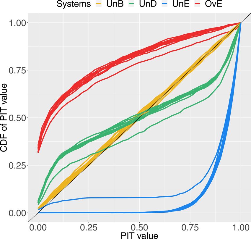
1034                            M. Cassagnole et al.: Impact of hydrological forecast quality on hydroelectric reservoirs

more than 80 % are operated by Électricité de France (EDF).         Among the data used in reservoir management and op-
EDF develops in-house forecasting systems to forecast river      eration, the water inflows to the reservoir, characterized by
discharges and reservoir inflows in catchments of sizes rang-    their time variability, are crucial if they are either observed
ing from a few tens to thousands of square kilometers. Most      hydrologic flows or forecasts. Streamflow forecasts provide
catchments are located in mountainous areas and are gov-         short- to long-term information on the possible scenarios of
erned by different hydrological regimes from glacio-nival to     inflows and, consequently, affect the decisions to be made
more pluvial-dominant runoff regimes. Forecasting systems        on releases and storage. The effectiveness of an optimiza-
allow one to anticipate hydrometeorological conditions from      tion model may thus depend on how good these forecasts
hours to days and months ahead. Over the years, investments      are. Murphy (1993) lists three main aspects that define if
have been made to develop deterministic and probabilistic        a forecast is good: consistency, quality and value. Forecast
forecast products that meet the requirements of being reli-      consistency relates to the correspondence between the fore-
able and accurate. Usefulness is ensured by constant interac-    cast and the forecaster’s best judgment, which depends on the
tion with users. However, questions remain: are investments      forecaster’s base knowledge. Forecast quality relates to how
in forecast quality rewarding in terms of economic benefits      close the forecast values (or the forecast probabilities) are to
and improved hydropower production management; and how           what actually happened. Forecast value relates to the degree
does forecast quality impact reservoir management and hy-        to which the forecast helps in a decision-making process and
dropower revenues?                                               contributes to realize an economic or other benefit.
   Operating a hydroelectric reservoir involves deciding            Forecast quality is often characterized by attributes, such
when it is more beneficial to produce energy (i.e., use the      as reliability, sharpness, bias and accuracy. It is often as-
water stored in the reservoir by releasing it through the tur-   sessed with numeric or graphic scores and independently of
bines of the power plant) and when it is more beneficial to      forecast value. When forecasts are affected by errors and dis-
store the water in the reservoir to use when demand (and         play biases or inaccuracies, they can be improved by apply-
electricity prices) are higher. Management decisions are also    ing statistical corrections, also called postprocessing tech-
affected by other roles the reservoir may have within inte-      niques, to the biased forecasts. Postprocessing is widely
grated river basin management (e.g., irrigation for agricul-     discussed in the literature (Ma et al., 2016; Crochemore
ture, flood control and drought relief) as well as by manage-    et al., 2016; Thiboult and Anctil, 2015; Pagano et al., 2014;
ment constraints (e.g., reservoir capacity and production ca-    Verkade et al., 2013; Trinh et al., 2013; Gneiting et al.,
pacity), which are specific to each reservoir. To help reser-    2005, 2007; Fortin et al., 2006) for deterministic and prob-
voir management decision-making, tools exist that model          abilistic (or ensemble-based) forecasts. It is also widely
the management problem and help to find the optimal se-          demonstrated that multiscenario ensemble forecasts provide
quence of releases in order to fulfill the management objec-     forecasts of better quality and enhanced potential usefulness
tives. In the literature, there are several optimization algo-   when compared to single-value deterministic forecasts, even
rithms used to manage hydroelectric reservoirs. Dobson et al.    when the mean of all ensemble members is used (Fan et al.,
(2019), Rani and Moreira (2010), Ahmad et al. (2014), Ce-        2015; Velázquez et al., 2011; Boucher et al., 2011; Roulin,
leste and Billib (2009) and Labadie (2004) carried out ex-       2007).
tensive reviews of the most common optimization methods.            While the analysis of forecast quality receives much at-
Three main classes of optimization algorithms that are ef-       tention, with numerous scores developed to quantify quality
ficient for optimizing reservoir management are (1) linear       gains when improving a forecasting system, the evaluation
and nonlinear programming (Arsenault and Côté, 2019; Yoo,        of forecast value remains a challenge. The value of a fore-
2009; Barros et al., 2003), (2) dynamic programming (Bell-       cast represents the benefits realized through the use of the
man, 1957) and its variants, deterministic dynamic program-      forecast in decision-making. It is therefore necessary to ac-
ming (DDP) (Haguma and Leconte, 2018; Ming et al., 2017;         quire knowledge on how decisions are made when informed
Yuan et al., 2016), stochastic dynamic programming (SDP)         by forecasts. In the context of hydroelectric reservoir man-
(Wu et al., 2018; Yuan et al., 2016; Celeste and Billib, 2009;   agement, the value of a forecast is often assessed by the per-
Tejada-Guibert et al., 1995), sampling stochastic dynamic        formance and benefits obtained from optimal management,
programming (SSDP) (Haguma and Leconte, 2018; Faber              when management objectives are satisfied and constraints are
and Stedinger, 2001; Kelman et al., 1990) and stochastic         respected (storage capacity and environmental constraints).
dual dynamic programming (SDDP) (Macian-Sorribes et al.,         It can be expressed (1) in terms of economic revenues, often
2017; Tilmant and Kelman, 2007; Tilmant et al., 2008, 2011;      associated with a monetary unit (Arsenault and Côté, 2019;
Pereira and Pinto, 1991), and (3) heuristic programming          Tilmant et al., 2014; Alemu et al., 2011; Faber and Stedinger,
(Macian-Sorribes and Pulido-Velazquez, 2017; Ahmed and           2001), and (2) in terms of utility, often associated with a pro-
Sarma, 2005). The choice among these algorithms depends          duction unit (Côté and Leconte, 2016; Desreumaux et al.,
on many factors, such as the stakes and objectives to address,   2014; Boucher et al., 2012; Tang et al., 2010).
as well as the configuration of the system and the data avail-      The analysis of the relationship between the quality of
able to parametrize and run the model.                           hydrometeorological forecasts and their economic value in

Hydrol. Earth Syst. Sci., 25, 1033–1052, 2021                                     https://doi.org/10.5194/hess-25-1033-2021
M. Cassagnole et al.: Impact of hydrological forecast quality on hydroelectric reservoirs                                     1035

the hydroelectric sector is more frequent in the context of           Lamontagne and Stedinger (2018) presented two statisti-
seasonal hydropower reservoir management. For example,             cal models to generate synthetic forecast values based on a
Hamlet et al. (2002) show that the benefits generated by the       time series of observed weekly flows. The synthetic fore-
use of seasonal forecasting for the management of a water          casts are then used in a simplified conceptual reservoir oper-
reservoir used for irrigation, hydropower production, nav-         ation framework where operators aim at keeping their reser-
igation, flood protection and tourism represent an average         voir level at a target level during summer. Hydropower ben-
increase in annual revenue of approximately USD 153 mil-           efits are maximized based on the weekly flows and benefits
lion per year. Boucher et al. (2012) studied the link between      are computed based on the assumption of constant electricity
forecast quality and value at shorter, days ahead, lead times.     prices. Forecast quality is evaluated using the coefficient of
The authors reforecast a flood event that occurred in the          determination as a measure of skill. The study showed that
Gatineau river basin in Canada due to consecutive rainfall         more accurate forecasts result in higher reservoir freeboard
events and evaluate the management of the Baskatong hy-            levels and reduced spills. It also highlighted the importance
dropower reservoir under different inflow forecast scenarios.      of using synthetic forecasts with varying precision to com-
They show that the use of deterministic or raw (without bias       pare the relative merit of different forecast products.
correction) ensemble streamflow forecasts does not affect the         Arsenault and Côté (2019) investigated the effects of sea-
forecast management value. However, the use of a postpro-          sonal forecasting biases on hydropower management. The
cessor to correct ensemble forecast biases lead to a better        study is based on the ensemble streamflow prediction (ESP)
reservoir management.                                              method, which uses historic precipitation and temperature
   In order to better understand the relationship between          time series to build possible future climate scenarios and
the quality of hydrometeorological forecasts and their value       force a hydrological model. The forecasts are issued at 120 d
through the management of hydroelectric reservoirs, some           time horizons. The authors apply a correction factor to the
studies have created synthetic, quality-controlled hydrolog-       ESP hydrometeorological forecasts, generating a positive
ical forecasts. The use of synthetic forecasts for reservoir       bias of +7 % (overestimation) and a negative bias of −7 %
management is, for example, implemented by Maurer and              (underestimation). The study is carried out on the Saguenay-
Lettenmaier (2004). The authors study the influence of syn-        Lac-St-Jean hydroelectric complex in Quebec, which con-
thetic seasonal 12-month hydrological forecasts on the man-        sists of five reservoirs. The authors also vary the manage-
agement of six reservoirs in the Missouri River basin in North     ment constraints by imposing, or removing, a minimum pro-
America. Synthetic forecasts are created by applying an er-        duction constraint on management. The study concludes that
ror to past observed flows (flows reconstructed over a 100-        more constrained systems tend to be more robust to forecast
year period). The error is defined according to the lead time      biases due to their reduced degree of freedom to optimize
(increasing error with lead time) and according to the level       the release/storage scheduling of inflows. Forecasts with a
of predictability the authors wanted to give to the synthetic      positive bias (overestimation) led to lower spill volumes than
forecast. Predictability is assessed by the correlation between    forecasts with a negative bias (underestimation). In addition,
past observed seasonal mean flows and the river basin ini-         it was shown that forecasts with a positive bias (overestima-
tial conditions. Four levels of predictability are defined ac-     tion) were correlated with a lower reservoir level.
cording to the variables considered in assessing the initial          For practical applications, the value of synthetic forecasts
conditions: (1) good predictability (climate variables, snow       is related to how the biases in these forecasts reflect the ac-
water equivalence and soil moisture are considered), (2) av-       tual biases encountered in operational forecasts. In opera-
erage predictability (only climate variables and snow water        tional hydrological forecasts, biases may vary according to
equivalence are considered), (3) poor predictability (only cli-    the time of the year, the magnitude of flows (different bi-
mate variables are considered) and (4) zero predictability (no     ases may be observed for high and low flows), the catch-
variables are considered). These levels of predictability are      ment and its climatic conditions, among other things. Ad-
expressed in terms of coefficients (the stronger the coeffi-       ditionally, forecast biases are often dependent on lead time.
cient, the higher the predictability), which are taken into ac-    Lamontagne and Stedinger (2018) emphasized that synthetic
count in the error of the synthetic forecast. The results of       forecasts should replicate the most important statistical prop-
this study draw two main conclusions: (1) synthetic fore-          erties (mean, variance and accuracy) of the real forecasts or
casts with better predictability generate the highest revenues     the specified properties of a potential forecast product to be
(closer to those of a perfect forecast system) and (2) the size    analyzed. Arsenault and Côté (2019) explained that they ex-
of the reservoir influences the value of the synthetic forecast    cluded larger variations of biases in their study since this
(for a large reservoir, the difference between the benefits of     would not be of additional help in exploring the behavior
the synthetic forecast with zero predictability and those of       of biases on the hydropower system operation of their case
the perfect forecast system represented by observed stream-        study.
flows are 1.8 %, compared to 7.1 % for a reservoir reduced by         Most of the studies in the literature deal with seasonal fore-
nearly a third of its capacity, which represents a difference of   casts, specific flood events or specific contexts of applica-
EUR 25.7 million in average annual revenues).                      tion, including single-site case studies. Furthermore, to the

https://doi.org/10.5194/hess-25-1033-2021                                       Hydrol. Earth Syst. Sci., 25, 1033–1052, 2021
1036 M. Cassagnole et al.: Impact of hydrological forecast quality on hydroelectric reservoirs
best of our knowledge, there have not been studies that tried located in the Cévennes mountains, where the hydrological
to untangle the influence of the different quality attributes regime is also marked by very low summer flows.
of a forecast on the management of reservoirs. Most of the Daily streamflow data come from the French database
existing studies either conclude that there is an overall link Banque HYDRO (Leleu et al., 2014). They are either natural
between the quality of hydrological forecasts and their eco- flows or, when the flows are influenced by existing dams, nat-
nomic value without specifying which quality attribute has uralized flows at the catchment outlet. In this study, they rep-
the greatest influence on the economic value or focus on a resent the inflows to the hydroelectric dams and are used to
single particular attribute. For instance, Stakhiva and Stew- create the synthetic hydrological forecasts of different qual-
art (2010) show that improving the reliability of hydrologi- ity for the period 2005–2008.
cal forecasting systems can improve hydroelectric reservoir
management. Côté and Leconte (2016) also mention the neg- 2.2 Generation of synthetic hydrological forecasts
ative impact of underdispersion of a hydrological forecast-
ing system on reservoir management. Other studies focus on In order to investigate the impact of the quality of the fore-
impacts of forecast accuracy on reservoir management, par- casts on the management of hydroelectric reservoirs, we cre-
ticularly when dealing with extreme events, such as floods ated time series of 7 d ahead synthetic daily streamflow fore-
or droughts (Turner et al., 2017; Anghileri et al., 2016; Kim casts of controlled quality for each studied catchment. For
et al., 2007). this, for a given day and lead time, we first generate a re-
The aim of this paper is to present a study that inves- liable 50-member ensemble forecast based on the observed
tigates the impact of quality attributes of short-term (7 d daily streamflow value and a parameterized log-normal dis-
ahead) hydrological forecasts on the management of hydro- tribution, and then we introduce biases on the generation pro-
electric reservoirs under different inflow conditions. For this, cesses. For a given day and lead time, the approach can be
we present a method for creating synthetic hydrological fore- described by the following two major steps:
casts of controlled quality and we apply the different fore- 1. Creation of synthetic reliable forecasts: we consider the
casting systems generated to a reservoir management model. synthetic ensemble forecast probability distribution as a
The model, based on a linear optimization algorithm, is de- log-normal distribution with two parameters: mean (µ)
signed to represent conceptual reservoirs and management and standard deviation (σ ). The standard deviation pa-
contexts with a simplified parametrization that takes into rameter is set as a function of a spread coefficient (D 2 )
account hypothetical reservoir physical parameters and the and the mean. In other terms, σ is expressed by a multi-
actual inflow variability from the upstream catchment area. plicative error around the mean (Eq. 1). The higher the
This framework allows us to investigate several sites and un- spread coefficient, the higher the standard deviation.
tangle the influence of different attributes of forecast quality
on hydroelectric production revenues. Our study is based on σ = D 2 × |µ| (1)
data from 10 catchments in France. In the following, Sect. 2
presents the case study areas, the data and methods used. Sec- The location parameter mean (µ) depends on the daily
tion 3 presents the results and discussions and is followed by observed streamflow. In probability theory, if a value X
Sect. 4, where conclusions are drawn. follows a log-normal distribution with parameters (µ,
σ ), the variable Y = log(X) follows a normal distribu-
tion with parameters (µ, σ ). The variate Z = Y −µσ fol-
lows a standard normal distribution of parameters µ = 0
2 Data and methods and σ = 1. For a probability 0 < p < 1, the quantile
function of the standard normal distribution returns the
2.1 Case study areas and streamflow data value z such that
This study is based on a set of 10 catchments located in the F (z) = P r(Z ≤ z) = p. (2)
southeast of France. They were selected to represent a vari-
ety of hydrological regimes and areas where the French elec- Considering that the variable X represents the observed
tric utility company EDF operates, or has interest in operat- streamflow, with Y = log(X), the quantile qp associ-
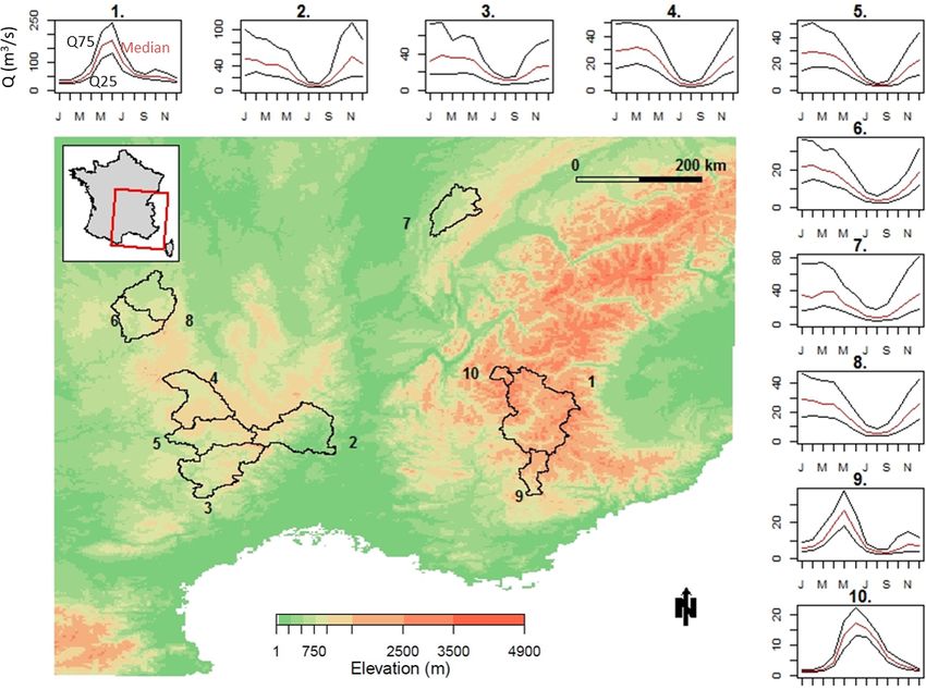
ing, hydroelectric dams. Figure 1 shows the location and hy- ated with the probability p is then
drological regimes of the studied catchments. Catchments 1,
log(X) − µ
9 and 10 are located in the French Alps. They are described = qp. (3)
by a snow-dominated hydrological regime, with peak flows σ
observed in spring due to snow melt. Catchment 7 is located
From Eq. (1), the log-normal mean µ is then given by
in the Jura mountains and its hydrological regime is domi-
nated by peak flows in winter followed by high flows also log(X)
in spring. The same is observed for catchments 2–6 and 8, µ= . (4)
1 + qp × D 2
Hydrol. Earth Syst. Sci., 25, 1033–1052, 2021 https://doi.org/10.5194/hess-25-1033-2021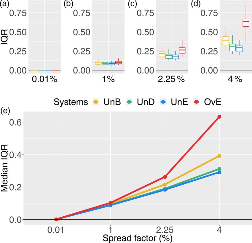
M. Cassagnole et al.: Impact of hydrological forecast quality on hydroelectric reservoirs                                                 1037

Figure 1. Location and hydrological regimes of the 10 studied catchments in France. Lines represent the 75th (upper black line), 50th (central
red line) and 25th (lower black line) percentiles of interannual daily flows (in m3 s−1 ), evaluated with observed streamflow data available for
the period 1958–2008.

     In order to guarantee the creation of a reliable ensem-                    forecasting centers of EDF is taken as reference. It is
     ble forecast, values of p are drawn randomly between 0                     based on a conceptual rainfall-runoff model (MORDOR
     and 1 from a uniform probability distribution for each                     model; Garçon, 1996) forced by the 50 members of the
     day and lead time. The sampling must thus be large                         meteorological ensemble forecasting system issued by
     enough to achieve an equal selection of probabilities                      the European Centre for Medium-Range Weather Fore-
     and obtain a reliable ensemble forecast. Finally, from                     casts (ECMWF). It produces 7 d ahead streamflow fore-
     the log-normal distribution with mean (µ) and standard                     casts daily. The quality of these operational forecasts,
     deviation (σ ), we randomly draw 50 members to gener-                      for a similar catchment dataset and evaluation period, is
     ate an ensemble.                                                           discussed in Zalachori et al. (2012).
     The steps above are carried out for each day of fore-
                                                                            2. Introduction of biases: from the previous step, we can
     cast and each lead time independently, which means
                                                                               generate ensemble forecasts that are reliable, sharp
     that temporal correlations can thus be lost. To retrieve
                                                                               (very close to the observed streamflows) and unbiased.
     correlated 7 d trajectories, we apply an approach based
                                                                               To deteriorate the quality of the forecasts, we implement
     on the ensemble copula coupling (ECC) postprocessing
                                                                               perturbations to be added to the generation process.
     methodology (Schefzik et al., 2013; Bremnes, 2008).
     The approach consists of rearranging the sampled val-                      To deteriorate the reliability of the synthetic forecasts,
     ues of the synthetic forecasts in the rank order struc-                    the values of p, which define the position of the ob-
     ture given by a reference ensemble forecasting system,                     servation in the probability distribution of the ensem-
     where physically based temporal patterns are present.                      ble forecast, are not taken randomly. This is done by
     Forecast members are ranked and the rank structure is                      introducing a reliability coefficient (R) as a power co-
     applied to the synthetic forecasts to create reordered                     efficient in the p value: p R . According to the value
     trajectories that match the temporal evolution of the                      taken by R, the random drawing will be biased (R 6= 1)
     reference forecasting system. In our study, the oper-                      or not (R = 1). We created synthetic ensembles with a
     ational ensemble forecasting system produced at the                        negative bias (0 < R < 1) and a positive bias (R > 1),

https://doi.org/10.5194/hess-25-1033-2021                                                Hydrol. Earth Syst. Sci., 25, 1033–1052, 2021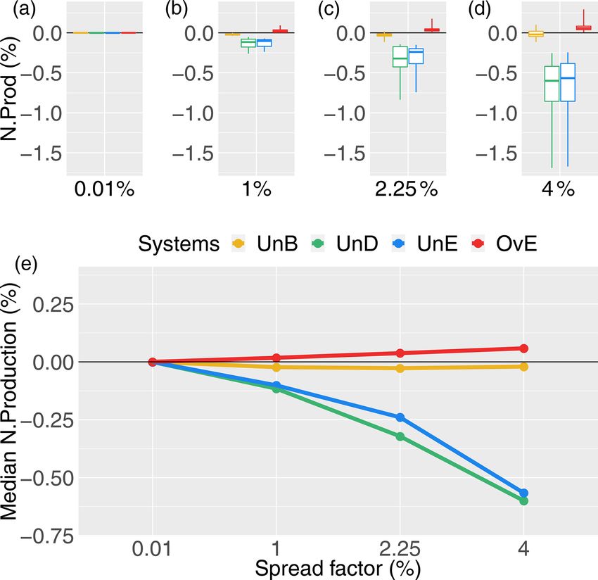
1038 M. Cassagnole et al.: Impact of hydrological forecast quality on hydroelectric reservoirs
which are associated with forecasts that underestimate 2.3 Reservoir management model
and overestimate the observations, respectively.
To generate underdispersed ensembles, the synthetic The reservoir management model is based on linear program-
generation is controlled so that high flows are under- ming (LP) to solve the optimization problem: maximize hy-
estimated and low flows are overestimated. In practice, dropower revenue under the constraints of maximum and
each daily observed streamflow is compared with the minimum reservoir capacities. Linear programming is one
quantiles 25 % and 75 % of the observed probability dis- of the simplest ways to quickly solve a wide range of lin-
tribution. If the daily observation is lower than the quan- ear optimization problems. The linear problem is solved by
tile 25 %, the p value is forced to be between 0 and 0.1. the open-source solver COIN Clp, which applies the sim-
If the daily observation is higher than the quantile 75 %, plex algorithm. The solver is called using PuLP, a Python
the p value is forced to be between 0.9 and 1. In this library for linear optimization. The model is an improvement
way, 50 % of the daily synthetic forecasts are forced to of a heuristic model of hydropower reservoir inflow manage-
under- or overestimate the observations. ment that was previously designed by EDF and INRAE for
research purposes. It defines the reservoir management rules
Finally, to deteriorate the sharpness and the accuracy,
at the hourly time step based on deterministic 7 d inflow fore-
the spread coefficient (D) is increased. Higher spread
casts and hourly time series of electricity prices.
coefficients will generate less sharp and accurate en-
Electricity prices in France have seasonal variability, with
semble forecasts. An ensemble forecast very close to the
higher prices in winter due to the higher electricity demand
observed streamflows is generated from the synthetic
for heating. They also vary within a week (lower prices are
ensemble forecasting model with a D coefficient equal
observed during weekends when industrial demand is lower)
to 0.01, corresponding to a spread factor of 0.01 %.
and within a day (higher prices are observed during peak de-
We then generated additional ensembles with D coef-
mand hours). In this study, we use the hourly energy price
ficients equal to 0.1, 0.15 and 0.2, which corresponds
time series for the period 2005–2008 from the EPEX-SPOT
to spread factors of 1 %, 2.25 % and 4 %. These are
market (https://www.epexspot.com/en, last access: 14 Febru-
low values compared to actual biases that can be found
ary 2021). This study period avoids the negative market
in real-world forecasts. However, since our synthetic
prices observed after 2008. Since we want to isolate the in-
generation model is based on a log-normal distribu-
fluence of the quality of inflow forecasts on the revenue, we
tion, the degree of skewness can increase fast as we in-
used observed prices instead of forecast prices.
crease D (and, consequently, as σ is increased), gener-
The 10 studied catchments define the inflows to 10 hy-
ating streamflows that are too high to be realistic and
droelectric reservoirs, which are conceptually parameterized
used in the reservoir management model.
as follows: given the focus of the study on 7 d inflow fore-
In summary, for each studied catchment and over the 4- casts, the storage capacity of each reservoir is defined as five
year study period, we generated a total of 16 synthetic en- times the historic mean daily flow; the maximum electricity
semble forecasting systems represented in Table 1 (4 main production capacity, which is related to production power, is
types to characterize biases × 4 spread factors to character- set at three times the historic mean daily flow; and the min-
ize sharpness). imum storage capacity is set at 0 Mm3 for each reservoir.
Each synthetic ensemble forecasting system was generated Given the historic mean daily flows of the studied catch-
daily with 50 members and up to 7 d of forecast lead time. ments, the conceptual sizes of the reservoirs vary between
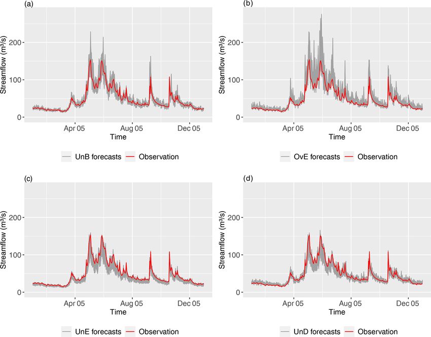
Figure 2 shows examples of the four synthetic ensemble fore- 3.18 and 34.22 Mm3 in this study. We do not use the ac-
casts generated for the 1 d lead time at catchment 1 (Fig. 1) tual reservoir dimensions and operational characteristics, al-
for the year 2005. It shows: though the inflows from the synthetic hydrological forecasts
– UnB (reliable and unbiased, Fig. 2a): forecasts uni- reflect the actual hydrological variability. For each synthetic
formly distributed around the observed flows, ensemble forecast, the reservoir management model is run
with the mean of the members of the ensemble. Running the
– OvE (overestimation, Fig. 2b): systematic positive bi- solver with each ensemble member and taking an average
ases towards forecasts that overestimate the observed decision would also be possible but would require additional
flows, investigation on the influence of extreme values of individual
members on the decision, which is beyond the scope of this
– UnE (underestimation, Fig. 2c): systematic negative bi-
paper.
ases towards forecasts that underestimate the observed
The LP optimization model defines, for each day, an opti-
flows,
mal release sequence (operation scheduling), which amounts
– UnD (underdispersed, Fig. 2d): flows greater than the to the water to be used to produce electricity. A rolling-
historic 75th percentile are underestimated and flows horizon optimization scheme is used. For each day, the op-
lower than the historic 25th percentile are overesti- timization problem is solved considering a 7 d window. It is
mated. informed by the 7 d synthetic streamflow forecast (ensemble
Hydrol. Earth Syst. Sci., 25, 1033–1052, 2021 https://doi.org/10.5194/hess-25-1033-2021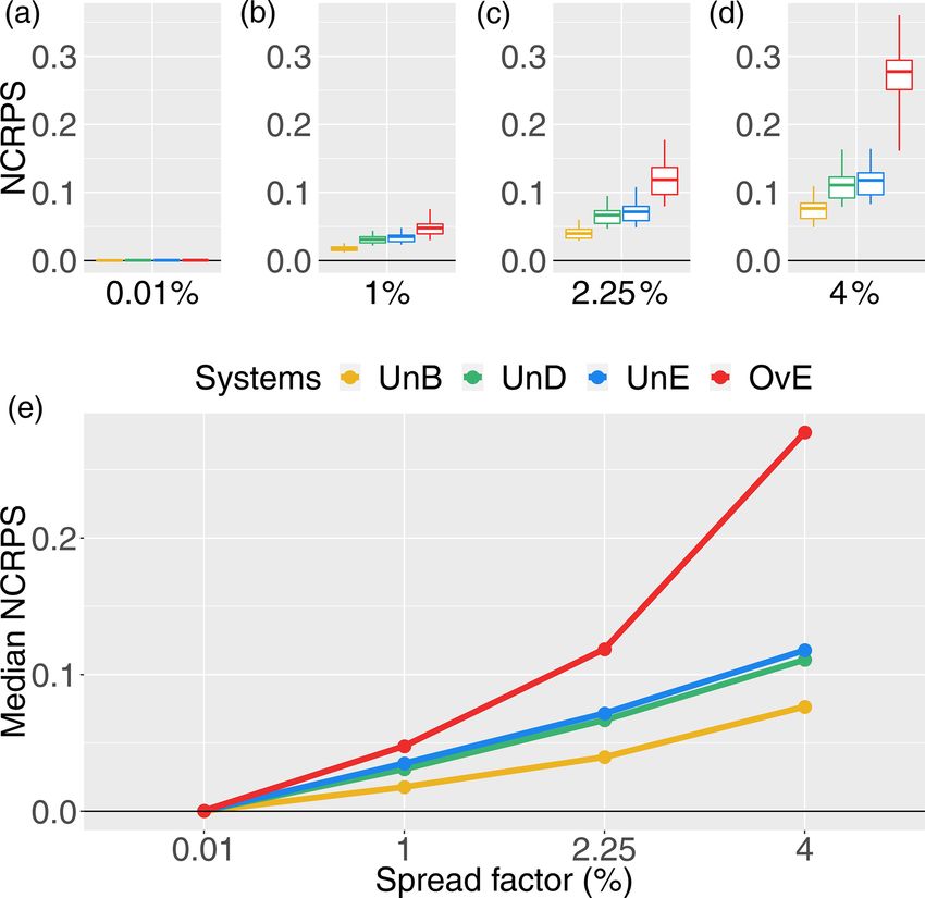
M. Cassagnole et al.: Impact of hydrological forecast quality on hydroelectric reservoirs                                                1039

Table 1. Summary of the 16 synthetic forecasting systems generated according to the four bias characterizations (UnB, OvE, UnE and UnD)
and the four sharpness characterizations (spread factors) applied.

                                                                           Bias characterization
  Sharpness characterization        UnB: reliable            OvE: overestimation            UnE: underestimation      UnD: underdispersed
  Spread factor (%)             0.01    1    2.25   4       0.01    1    2.25    4          0.01   1    2.25   4      0.01    1   2.25    4

Figure 2. Illustration of the synthetic forecasts generated: (a) UnB (reliable and unbiased forecasts), (b) OvE (forecasts that overestimate),
(c) UnE (forecasts that underestimate) and (d) UnD (underdispersed forecasts). The example is for catchment 1 (Fig. 1) and the 1 d forecasts
of 2005. The spread factor used for this figure is 2.25 %.

mean) and the hourly electricity prices. The algorithm max-              fied according to the objective function below, which is max-
imizes the hydropower revenue, searching for an optimal re-              imized over a week for each day of the study period:
lease sequence over the week. It tries to use all the incoming                  H −1
volume to produce electricity, thus maximizing the imme-
                                                                                X
                                                                         max           ph × ρ × q h ,                                     (5)
diate benefits of electricity generation. We did not use final                  h=0
water values to account for the state of the reservoir storage
at the end of the 7 d optimization period. However, we im-               where h refers to the hour of the week (in total, H = 168 h);
plemented the weekly production as a soft constraint, which              ph refers to the hourly electricity price at hour h; ρ refers to
should not be higher than the weekly volume of water enter-              the efficiency of the power plant, in MWh m−3 s−1 , which
ing the reservoir. This prevents the model from emptying the             is a constant equal to 1 MWh m−3 s−1 in this study; and
reservoirs at the end of the period.                                     qh refers to the release in m3 s−1 used for the production at
   The main objective of the reservoir management model                  hour h.
is to maximize hydropower revenue while meeting the con-                    Mayne et al. (2000) classify management constraints into
straints of the reservoir. The management objective is quanti-           two categories: hard constraints and soft constraints. Dobson
                                                                         et al. (2019) define these constraints as follows: “Hard con-

https://doi.org/10.5194/hess-25-1033-2021                                                  Hydrol. Earth Syst. Sci., 25, 1033–1052, 2021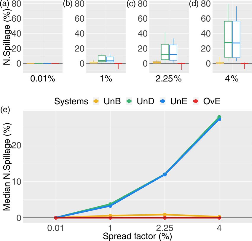
1040                                  M. Cassagnole et al.: Impact of hydrological forecast quality on hydroelectric reservoirs

straints are those constraints that cannot be violated under         optimal command of releases obtained during the optimiza-
any circumstance and typically represent physical limits [. . . ]    tion phase to the first day (there is no re-optimization). At
Soft constraints, instead, are those constraints that should not     this phase, it may happen that the observed inflows are very
be violated but that are not physically impossible to break.”        different from the forecast inflows used for the optimization
In our experiment, the maximum capacity is a soft constraint,        and, due to the management constraints, it is not possible to
while the minimum capacity is defined as a hard constraint.          follow the optimal command. In this case, the rule is modi-
When a major event occurs and the reservoir does not have            fied to allow the operations to be carried out within the stor-
the storage capacity required to store the inflow volume, the        age constraints. When the management rule at one hour h
maximum reservoir capacity constraint is violated. There are         induces a violation of the minimum storage constraint, the
penalty terms (associated with spills and minimum volumes)           release is decreased until the constraint is respected. On the
in the cost function, which intervene in the objective function      other hand, when a volume of water is spilled, the release is
during the optimization. Penalties are based on the order of         increased. We note that, in this case, the modified manage-
magnitude of the gains per hm3 (taking the maximum elec-             ment rule does not always avoid discharge and a volume of
tricity price into account). The minimum volume penalty is           spilled water may occur.
calculated to always be greater than the potential gains, and           The volume obtained at the end of the 24 h simulation
the spill penalty is 10 times the minimum volume penalty.            phase is used to update the initial volume of the reservoir
For instance, for a gain of 8 per hm3 , the order of magni-          for the next forecast day and optimization. This is done in
tude will be 1; the power to 10, zero; the minimum volume            a continuous loop over the entire 4-year study period (2005–
penalty, 10; and the spill penalty, 100. The storage constraints     2008) for each catchment and for the 16 synthetic streamflow
and the temporal evolution of the stock are quantified as            forecasts of different forecast quality. At the end, the amount
                                                                     of hourly electricity produced is multiplied by the price (in
vhmin ≤ vh ≤ vhmax                                            (6)    Euro per MWh) to obtain the revenue. The impact of forecast
vh = vh−1 + K (ah − qh ) ,                                    (7)    quality on the revenue (economic value) is then assessed.

where vhmin and vhmax represent, respectively, the minimum
                                                                     2.4   Evaluation of forecast quality
and maximum volume of the reservoir at hour h in Mm3 ;
ah represents the forecast inflow at hour h in m3 s−1
and K represents the conversion constant from m3 s−1                 In terms of forecast quality, we focus on assessing the relia-
to Mm3 h−1 (equal to 0.0036).                                        bility, sharpness, bias and accuracy of the forecasts.
   The optimization is also constrained by the maximum pro-             The reliability is a forecast attribute that measures the
duction capacity, which is considered a hard constraint. Pro-        correspondence between observed frequencies and forecast
duction therefore cannot exceed the maximum production               probabilities. It can be measured by the probability integral
capacity:                                                            transform (PIT) diagram (Gneiting et al., 2007; Laio and
                                                                     Tamea, 2006) at each forecast lead time. The diagram repre-
0 ≤ qh ≤ qmax ,                                               (8)    sents the cumulative frequency of the values of the predictive
                                                                     (forecast) distribution function at the observations. A reliable
where qh refers to the release in m3 s−1 at hour h and               forecast has a PIT diagram superposed with the diagonal (0–
qmax refers to the maximum release (associated with the max-         0 to 1–1). It means that the observations uniformly fall within
imum production capacity).                                           the forecast distribution. A forecasting system that overesti-
   Furthermore, the optimization is constrained by the               mates the observations is represented by a curve above the di-
weekly release for electricity production, which cannot be           agonal. If the PIT diagram is under the diagonal, it indicates
higher than the weekly inflows. This constraint is considered        that observations are systematically underestimated. A PIT
a soft constraint. It has been implemented for this research         diagram that tends to be horizontal means that the forecasts
management model and is not representative of the real op-           suffer from underdispersion (i.e., observations often fall in
erational constraints. It can be expressed as                        the tail ends of the forecast distribution). On the other hand,
                                                                     a PIT diagram that tends to be vertical means that the fore-
H −1                     H −1
X                        X                                           casts are overdispersed.
       (K × qh ) ≤ A =          (K × ah ) ,                   (9)
h=0                      h=0
                                                                        The sharpness of a forecast corresponds to the spread of
                                                                     the ensemble forecast members. It is an attribute indepen-
where A represents the cumulative weekly inflows.                    dent of the observations, which is therefore specific to each
   When applying the model, after the optimization phase             forecasting system. To evaluate the sharpness of a forecast
and once the operation schedule is defined for the coming            for each lead time, the 90 % interquantile range (IQR) can
week, it simulates the management of the reservoir with the          be used (Gneiting et al., 2007). It corresponds to the differ-
actual observed inflows over the release schedule defined for        ence between the 95th quantile and the 5th quantile of all en-
the first 24 h. This simulation phase consists of applying the       semble members. The IQR score is evaluated for each fore-

Hydrol. Earth Syst. Sci., 25, 1033–1052, 2021                                         https://doi.org/10.5194/hess-25-1033-2021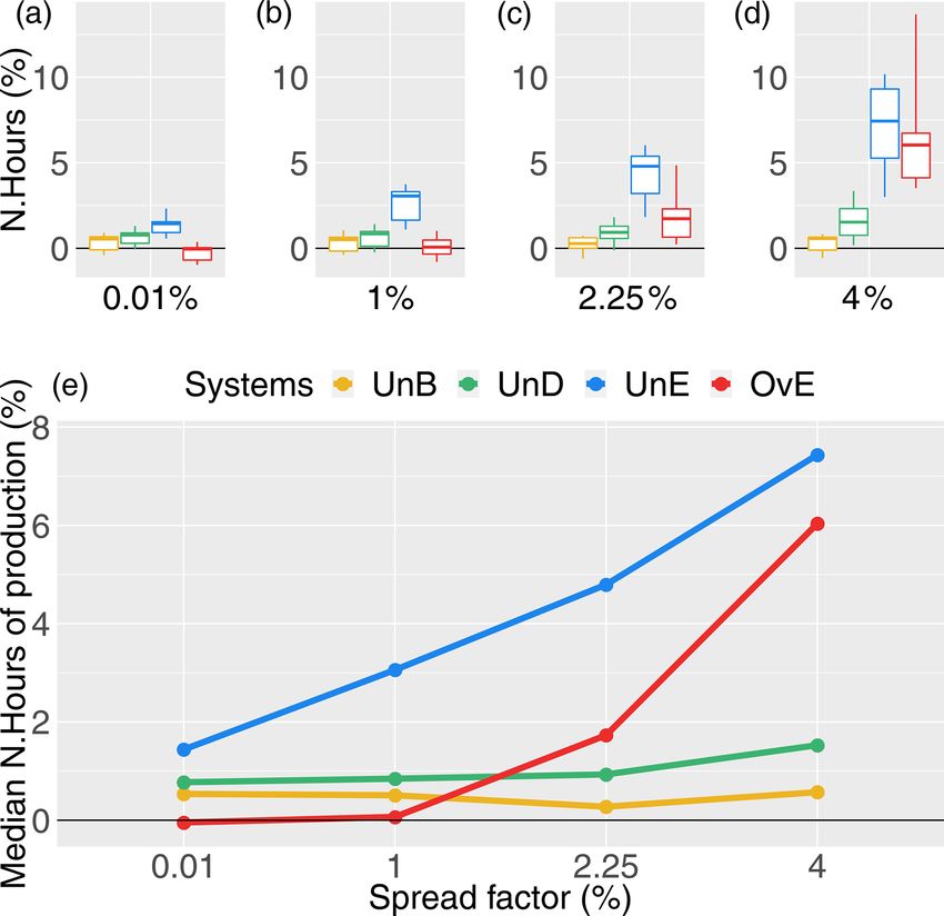
M. Cassagnole et al.: Impact of hydrological forecast quality on hydroelectric reservoirs 1041
cast day and then averaged over the entire study period. The
smaller the IQR, the sharper the forecast.
The forecast bias measures the average error of a forecast
in relation to the observation over a given time period. Bias
measurement is used to detect positive (forecasts greater than
observations) or negative (forecasts lower than observations)
biases. To evaluate the bias of the synthetic ensemble stream-
flow forecasts, the percent bias (Pbias) is computed for each
day i and lead time (Fan et al., 2016; Waseem et al., 2015). It
compares the daily observation o with the daily mean of the
ensemble forecast m. The Pbias score is then averaged over
the entire study period of N forecast days:
N
P
(mi − oi )
i=1
Pbias = 100 · . (10)
N
P
oi
i=1
The Pbias is negative (positive) when forecasts underestimate
(overestimate) the observations.
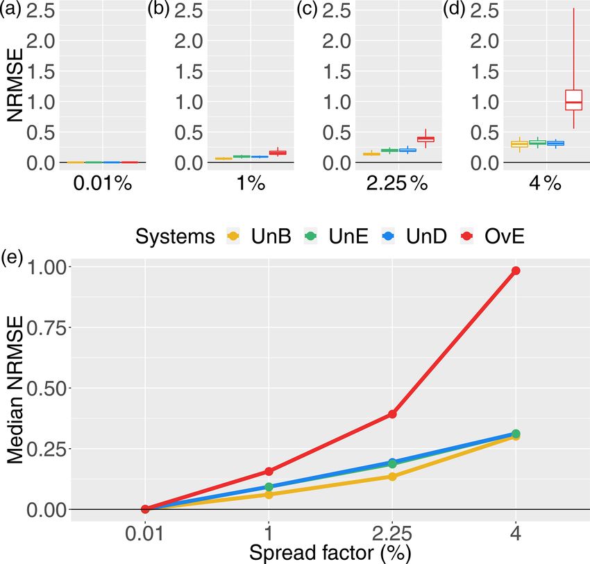
The accuracy of a forecast represents the difference be- Figure 3. IQR score for 1 d ahead synthetically generated forecasts
tween an observed value and an expected forecast value. It of different quality: unbiased system (UnB, yellow), underdispersed
is often assessed with the root mean square error (RMSE), system (UnD, green), underestimating system (UnE, blue) and over-
which corresponds to the square root of the mean square er- estimating system (OvE, red). Systems are based on ensembles gen-
ror. In the case of an ensemble forecast, the average of the erated with four different spread factors (0.01 %, 1 %, 2.25 % and
ensemble forecast is often used to assess the accuracy of the 4 %). (a–d) Boxplots represent the maximum value, percentiles 75,
forecasting system. In this study, the RMSE is normalized 50 and 25, and minimum value over the 10 studied catchments.
with the standard deviation (SD) of the observations to allow (e) Median score value.
comparison among different catchments:
RMSE
NRMSE = . (11)
SDobs ensemble hydrological forecasting system in terms of sharp-
The lower the NRMSE, the more accurate the forecast is. ness (Fig. 3), reliability (Fig. 4), systematic bias (Fig. 5), ac-
Finally, we evaluated the overall forecast quality of each curacy (Fig. 6) and overall quality (Fig. 7). The quality of
forecasting system with the continuous ranked probability the synthetic ensemble forecasts is presented at the 1 d lead
score (CRPS) (Hersbach, 2000). It compares the forecast time only, since, by construction, the quality of the synthetic
distribution to the observation distribution (a Heaviside step forecasts does not vary according to the lead time. In all the
function at the observation location) over the evaluation pe- figures except Fig. 4, the top graphs show, in the form of box-
riod. The score is better if the probability distribution of the plots (maximum value, percentiles 75, 50 and 25, and mini-
forecasts is close to that of the observations. The lower the mum value), the distribution of the scores of quality for the
CRPS, the better the forecasts are. In this study, the CRPS 10 catchments of the study. The bottom graphs highlight the
is also normalized with the SD of the observations to reduce evolution of the median score (percentile 50). In both graphs,
the impact of the catchment size on this score (Trinh et al., the results are presented for four spread factors (0.01 %, 1 %,
2013): 2.25 % and 4 %).
Figure 3 shows the effect of the increase in the spread fac-
CRPS tor on the sharpness score (IQR) of each synthetic ensemble
NCRPS = . (12)
SDobs forecasting system. The evolution of IQR values for the unbi-
ased system (UnB) can be used as a reference of expected im-
pacts; the dispersion of the ensemble system increases when
3 Results and discussions the spread factor increases. Therefore, the model designed
for the generation of synthetic ensemble forecasts of con-
3.1 Quality of the generated synthetic hydrological trolled quality works as expected in terms of spread varia-
forecasts tions. Additionally, we also observe that the IQR scores are
not very different among the forecasting systems and the
In order to validate the model used to generate synthetic fore- studied catchments for the smaller spread factors. To differ-
casts of controlled quality, we evaluated the quality of each entiate the ensemble systems in terms of their sharpness, it
https://doi.org/10.5194/hess-25-1033-2021 Hydrol. Earth Syst. Sci., 25, 1033–1052, 2021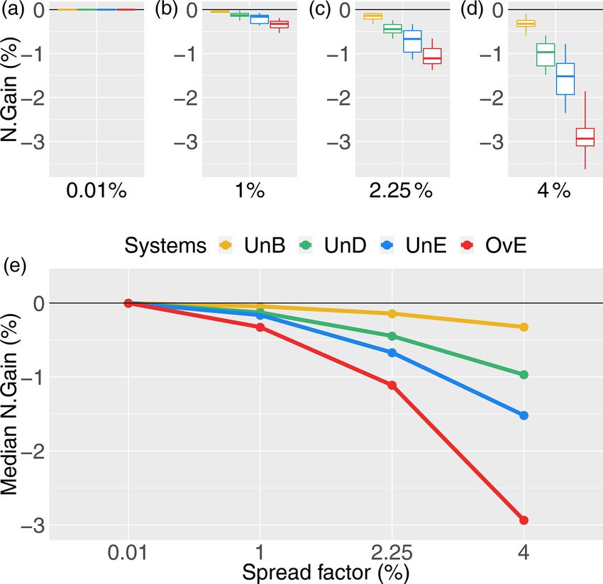
1042                               M. Cassagnole et al.: Impact of hydrological forecast quality on hydroelectric reservoirs

Figure 4. PIT diagram for 1 d ahead synthetically generated fore-
casts of different quality: unbiased system (UnB, yellow), underdis-
persed system (UnD, green), underestimating system (UnE, blue)
and overestimating system (OvE, red). For each system, each line
represents one of the 10 studied catchments. Forecasts are based on
ensembles generated with a 4 % spread factor.
                                                                       Figure 5. Pbias score for 1 d ahead synthetically generated fore-
                                                                       casts of different quality: unbiased system (UnB, yellow), underdis-
is thus necessary to have a spread factor greater than 1 %             persed system (UnD, green), underestimating system (UnE, blue)
in the synthetic forecast generator model, regardless of the           and overestimating system (OvE, red). Systems are based on en-
catchment location or the bias of the system. The intercatch-          sembles generated with four different spread factors (0.01 %, 1 %,
                                                                       2.25 % and 4 %). (a–d) Boxplots represent the maximum value, per-
ment difference as well as the differences among the fore-
                                                                       centiles 75, 50 and 25, and minimum value over the 10 studied
casting systems increase as the spread factor increases. These
                                                                       catchments. (e) Median score value.
differences also reflect the way the synthetic ensemble fore-
casts were generated. The implementation of a reliability bias
towards overestimation of streamflows (OvE system) has a
strong impact on sharpness. IQR score values are the highest           of the PIT values as expected in a probabilistically calibrated
for this system, particularly when the spread factor is high.          ensemble forecasting system. The forecast deficiencies of the
The spread of the forecasts is thus the highest for this sys-          biased-generated systems are illustrated in the PIT diagram
tem. This can be explained by the fact that, by construc-              by their distance to the uniformity of a reliable system. The
tion, there is no physical upper limit imposed to the over-            forms of the curves reflect well the underdispersion of the
estimation of streamflows. On the contrary, for the system             system UnD, as well as the overestimation and the underes-
that was generated to present a bias towards underestima-              timation of the systems OvE and UnE, respectively.
tion (UnE), the lower limit physically exists and corresponds             The reliable system (UnB) also shows zero to very low
to zero flows. This explains why this system shows low IQR             percent bias, as illustrated in Fig. 5. For this system, a slight
scores even at the highest spread factor. In the underdispersed        positive bias appears when using a 4 % spread factor. The fact
system (UnD), the low flows are overestimated, while the               that the increase in spread leads to a slight positive bias (over-
high flows are underestimated. By construction, the forecasts          estimation), even when the system is generated to be prob-
are thus more concentrated and the dispersion of this system           abilistically unbiased, may be the consequence of the skew-
tends to be small. This is also reflected in Fig. 3, where the         ness of the log-normal distribution used in the forecast gener-
values of IQR for the UnD system are very close to those of            ation model, which increases as the spread increases and may
the UnE system.                                                        result in the generation of some very high values, affecting
   The evaluation of reliability is shown in Fig. 4. The PIT di-       the median bias. This impact is however much smaller com-
agram of each catchment is represented (lines) for the higher          pared to the impact of adding biases to the reliable forecasts.
spread factor only (4 %), when the differences in the quality          From Fig. 5, we can see a strong positive bias for the system
of the forecasting systems are higher. The lines in the PIT            that tends to overestimate streamflow observations (37 % of
diagram clearly show the effectiveness of the forecast gen-            median Pbias value for OvE and spread factor of 4 %) and a
erator model to introduce reliability biases in the unbiased           negative bias for the system that tends to underestimate them
forecasting systems of all catchments. The cumulative distri-          (up to −18 % of median Pbias value for the UnE system). We
butions of the PIT values of the unbiased systems (UnB) are            also observe that there are larger differences in Pbias values
located around the diagonal, showing a uniform distribution            among catchments in the OvE forecasting system, particu-

Hydrol. Earth Syst. Sci., 25, 1033–1052, 2021                                            https://doi.org/10.5194/hess-25-1033-2021
M. Cassagnole et al.: Impact of hydrological forecast quality on hydroelectric reservoirs 1043
Figure 6. NRMSE score for 1 d ahead synthetically generated fore- Figure 7. NCRPS score for 1 d ahead synthetically generated fore-
casts of different quality: unbiased system (UnB, yellow), underdis- casts of different quality: unbiased system (UnB, yellow), underdis-
persed system (UnD, green), underestimating system (UnE, blue) persed system (UnD, green), underestimating system (UnE, blue)
and overestimating system (OvE, red). Systems are based on en- and overestimating system (OvE, red). Systems are based on en-
sembles generated with four different spread factors (0.01 %, 1 %, sembles generated with four different spread factors (0.01 %, 1 %,
2.25 % and 4 %). (a–d) Boxplots represent the maximum value, per- 2.25 % and 4 %). (a–d) Boxplots represent the maximum value, per-
centiles 75, 50 and 25, and minimum value over the 10 studied centiles 75, 50 and 25, and minimum value over the 10 studied
catchments. (e) Median score value. catchments. (e) Median score value.
ble mean. This may be linked to the fact that the RMSE is
larly at spread factor of 4 % (Pbias values vary from 25 % to based on absolute values of the errors and is not sensitive
75 %). A negative bias is observed for underdispersed fore- to the direction of the error (as in Pbias). Also, the fact that
casts (−11.5 % of median Pbias value for UnD and spread larger differences have a larger effect on RMSE, given that
factor of 4 %). The values of Pbias for the OvE and UnD it is based on the square root of the average of squared er-
systems are close to each other and present the same signal. rors, the high streamflow values generated in the unbiased
This indicates that, in the UnD forecasting system, the im- system when using the higher spread factor penalize this sys-
pact of the underestimation of high flows in the percent bias tem, leading to RMSE scores very close to the scores of the
is higher than the impact of the overestimation of low flows. biased UnD and UnE systems, where high streamflow fore-
The resemblance between the two synthetic systems is also cast values tend to occur less often. Finally, we note that the
illustrated in Fig. 2. Finally, in all biased generated systems, range of NRMSE values of the OvE system comprises the
the higher the spread factor, the higher the absolute value of range of normalized RMSE values found by Zalachori et al.
the Pbias of the system. (2012) (NRMSE ranging from 1.7 to 2.4) when analyzing
The evaluation of the NRMSE (accuracy, Fig. 6) and the raw (without bias correction) operational forecasts over a
NCRPS (overall forecast quality, Fig. 7) scores also illus- similar dataset of catchments.
trates the impact of introducing biases in a reliable ensem-
ble streamflow forecasting system. Overestimation leads to 3.2 Economic value of the generated synthetic
the worst scores and the highest differences in performance hydrological forecasts
among catchments. Systems generated with underestimation
and underdispersion biases have very similar scores, reflect- The value of the different forecasting systems is assessed
ing their similarity when high peak flows are reduced (see based on the total economic revenue obtained from the hy-
Fig. 2). For all systems, scores get worse when increasing dropower reservoir operation when using, on a daily basis,
the spread factor (i.e., the ensemble spread). Although bet- each system’s 7 d forecasts as input to the reservoir manage-
ter for the unbiased and reliable system (UnB), the accu- ment model (LP optimization) over the study period (2005–
racy score (NRMSE) does not strongly differentiate the UnB, 2008). The revenue obtained with each synthetic forecast-
UnD and UnE systems in terms of accuracy of the ensem- ing system is then evaluated against the revenue obtained us-
https://doi.org/10.5194/hess-25-1033-2021 Hydrol. Earth Syst. Sci., 25, 1033–1052, 20211044 M. Cassagnole et al.: Impact of hydrological forecast quality on hydroelectric reservoirs
spread increases, the quality (sharpness, accuracy, reliability
and overall quality) decreases and the value (percentage gain
in revenue) decreases.
Figure 8 and the analysis of synthetic forecast quality
(Figs. 3–7) clearly show that the forecasting system display-
ing the worst scores in terms of forecast quality is also the
one that displays the lowest economic value (system OvE,
red line in Fig. 8). In the ranges and within the conditions
of our experiment, a forecast system that, in median values,
overestimates streamflows at about 30 % (Pbias) generates a
loss in revenue of up to 3 %, compared to the revenue gener-
ated by a forecasting system that perfectly forecasts the ob-
served inflows to the reservoir. Similarly, the unbiased sys-
tem (UnB), which has the best quality among the synthetic
forecasting systems (reliability, bias and overall quality), is
the system that provided hydropower revenues the closest to
the revenues of a perfect system. The second best system in
terms of economic value is the system that suffers from un-
derdispersion (UnD). Although, in terms of forecast quality,
this system ranks closely to the forecast system that underes-
Figure 8. Percentage gain in hydropower revenue (N. Gain in %) timates inflows (UnE), it performs, in median values, about
for synthetically generated forecasts of different quality: unbiased 0.5 % points better in terms of economic gains. The systems
system (UnB, yellow), underdispersed system (UnD, green), un- that under- and overestimate inflows (UnE and OvE, respec-
derestimating system (UnE, blue) and overestimating system (OvE, tively) are those that show a steeper rate of loss in economic
red). Systems are based on ensembles generated with four different revenue as the spread of the forecasts increases. When mov-
spread factors (0.01 %, 1 %, 2.25 %, and 4 %). (a–d) Boxplots rep- ing from a spread factor of 2.25 % to a spread factor of 4 %,
resent the maximum value, percentiles 75, 50 and 25, and minimum
the median percentage gains of the system UnE move from
value over the 10 studied catchments. (e) Median value.
−0.67 % to −1.5 %, while for the system OvE, it moves from
−1 % to −3 %. Notably, the overall rank in economic value
of the synthetic forecasting systems is similar to their rank in
ing a reference system. This reference system is given by quality according to the Pbias and the NCRPS scores.
the observed streamflows. It is thus equivalent to a “perfect
forecasting system”, where the forecasts are always identi- 3.3 Influence of forecast bias on the total amount and
cal to the observed inflows. Hence, the maximum revenue is hours of electricity production
obtained by the reference system. The gain in revenue ob-
tained for each synthetic system is expressed as the percent- The economic value of the synthetic forecasts is assessed
age gain in relation to the revenue of the reference system by the gains of revenue generated when using a given fore-
(N. Gain in %). This percentage gain is therefore negative casting system as inflow to the reservoir management model.
(i.e., a percentage of loss in relation to the reference). The re- Revenues (in euros) are calculated by multiplying the hourly
sults obtained are shown in Fig. 8. The graph on top shows, electricity production (MW) by the electricity price (euro
in boxplots, the distribution of the percentage gains (maxi- per MWh) at the time of production. It is not enough to pro-
mum value, percentiles 75, 50 and 25, and minimum value) duce a large amount of electricity to increase revenues. It is
of the 10 studied catchments. The graph at the bottom high- also necessary to optimally place the production at the best
lights the median gain. Both graphs show the gain for each hours (i.e., when the prices are higher). Here, we investigate
synthetic forecast system of controlled quality and as a func- how each synthetic forecasting system influences the total
tion of the spread factor used to generate the forecasts. production and number of hours of electricity produced over
The economic revenues of the different forecasting sys- the study period. Figure 9 shows the normalized total pro-
tems are very similar for the smaller spread factors. The duction of each synthetic forecasting system, while Fig. 10
difference in economic value between the synthetic forecast shows the normalized number of hours of production over
systems widens with the increase in the spread factor. More- the entire period. Both are expressed in terms of percentage
over, the percentage gains show a clear tendency to decrease of the total production (N. Production in % in Fig. 9) or of
as the spread factor increases. A given forecasting system the total hours of production (N. Hour of production in %
will lose more revenue in comparison with the reference per- in Fig. 10) of the reference system (i.e., the perfect system,
fect system as it becomes more dispersed. This observation is where forecasts are equal to observations).
in line with the analysis of the quality of the systems: as the
Hydrol. Earth Syst. Sci., 25, 1033–1052, 2021 https://doi.org/10.5194/hess-25-1033-2021You can also read