Carbon dioxide fluxes and carbon balance of an agricultural grassland in southern Finland - Biogeosciences
←
→
Page content transcription
If your browser does not render page correctly, please read the page content below

Biogeosciences, 18, 3467–3483, 2021
https://doi.org/10.5194/bg-18-3467-2021
© Author(s) 2021. This work is distributed under
the Creative Commons Attribution 4.0 License.

Carbon dioxide fluxes and carbon balance of an agricultural
grassland in southern Finland
Laura Heimsch1 , Annalea Lohila1,2 , Juha-Pekka Tuovinen1 , Henriikka Vekuri1 , Jussi Heinonsalo1,3 , Olli Nevalainen1 ,
Mika Korkiakoski1 , Jari Liski1 , Tuomas Laurila1 , and Liisa Kulmala1,3
1 Finnish  Meteorological Institute, P.O. Box 503, 00101 Helsinki, Finland
2 Institute for Atmospheric and Earth System Research, Physics, University of Helsinki,
P.O. Box 64, 00014 University of Helsinki, Finland
3 Institute for Atmospheric and Earth System Research, Forest Sciences, University of Helsinki,

P.O. Box 27, 00014 University of Helsinki, Finland

Correspondence: Laura Heimsch (laura.heimsch@fmi.fi)

Received: 11 November 2020 – Discussion started: 30 November 2020
Revised: 29 April 2021 – Accepted: 9 May 2021 – Published: 10 June 2021

Abstract. A significant proportion of the global carbon emis-    et al., 2009, 2017; Lal, 2016; Paustian et al., 2000; Smith,
sions to the atmosphere originate from agriculture. There-       2008). Currently, agriculture is responsible for more than
fore, continuous long-term monitoring of CO2 fluxes is es-       10 % of the global anthropogenic greenhouse gas (GHG)
sential to understand the carbon dynamics and balances of        emissions to the atmosphere (Le Quéré et al., 2017). Soil
different agricultural sites. Here we present results from a     type and properties, vegetation, climate, and weather condi-
new eddy covariance flux measurement site located in south-      tions as well as management practices all have a considerable
ern Finland. We measured CO2 and H2 O fluxes at this agri-       effect on the carbon fluxes and balances of agroecosystems
cultural grassland site for 2 years, from May 2018 to May        (Bolinder et al., 2010; Gomez-Casanovas et al., 2012; Jensen
2020. In particular the first summer experienced prolonged       et al., 2017; Lorenz and Lal, 2018; Singh et al., 2018). Fre-
dry periods, which affected the CO2 fluxes, and substantially    quent ploughing, monocropping and intensive use of agro-
larger fluxes were observed in the second summer. During the     chemicals are the main contributors to the loss of SOM and
dry summer, leaf area index (LAI) was notably lower than in      the resulting carbon dioxide (CO2 ) emissions from land use
the second summer. Water use efficiency increased with LAI       (Ceschia et al., 2010; Reinsch et al., 2018; Yang et al., 2019).
in a similar manner in both years, but photosynthetic capac-     A change from conventional and intensive agricultural prac-
ity per leaf area was lower during the dry summer. The an-       tices to regenerative and holistic farm management provides
nual carbon balance was calculated based on the CO2 fluxes       a substantial climate change mitigation potential (Lal, 2016).
and management measures, which included input of carbon          Increasing the amount of SOM in agroecosystems by apply-
as organic fertilizers and output as yield. The carbon balance   ing enhanced management practices, such as lighter tillage,
of the field was −57 ± 10 and −86 ± 12 g C m−2 yr−1 in the       continuous plant cover, rotational grazing, agroforestry, in-
first and second study years, respectively.                      creased biodiversity and cover cropping, would not only help
                                                                 to mitigate climate change but also to restore soil quality and
                                                                 fertility. In particular managed grasslands as part of agricul-
                                                                 tural systems have a high potential for substantial soil car-
1   Introduction                                                 bon sequestration (Soussana et al., 2010; Gilmanov et al.,
                                                                 2010; Yang et al., 2019). The importance of increasing soil
Conventional and intensive agricultural practices cause sig-     organic carbon (SOC) content of agricultural soils has re-
nificant carbon emissions while diminishing the soil organic     cently attained more attention, and the “4 per mille Soils for
matter (SOM) content. This leads to a reduction of soil qual-    Food Security and Climate” initiative was launched at the
ity and health (e.g. Houghton and Nassikas, 2017; Le Quéré

Published by Copernicus Publications on behalf of the European Geosciences Union.
3468                        L. Heimsch et al.: CO2 fluxes and C balance of an agricultural grassland in southern Finland

21st Conference of the Parties to the United Nations Frame-           Better understanding of climatic impacts of agriculture
work Convention on Climate Change in Paris in 2015 (Mi-            and the effects of improved practices from the perspective of
nasny et al., 2017). The aim of this initiative is to increase     soil health and vitality is needed in order to develop tools for
the soil carbon stock on all land surfaces in the upper 2 m on     improved environmental management of these ecosystems.
average by 0.4 % annually. The possible increase in carbon         Continuous long-term measurements of the atmosphere–
content is largely dependent on the soil properties, e.g. clay     ecosystem fluxes are needed to identify the key factors af-
content (Johannes et al., 2017; Minasny et al., 2017). This        fecting carbon dynamics of different ecosystems, to quan-
would be enough to sequester carbon from the atmosphere            tify the resulting carbon balance and its components, and to
by an amount equivalent to the annual anthropogenic GHG            verify soil carbon and ecosystem models. Moreover, high-
emissions. However, the initiative states that the most poten-     quality GHG flux data are needed for a reliable, global mea-
tial SOC increases can be achieved on managed agricultural         suring, reporting and verification system of agricultural car-
lands. In that case, the “4 per 1000” means increasing SOC         bon fluxes and soil carbon sequestration and stability (Smith
at the top 1 m layer of agricultural soils by 0.4 % annually.      et al., 2020).
That would effectively offset approximately 20 %–35 % of              The eddy covariance (EC) method is widely used for mea-
the global GHG emissions.                                          suring CO2 and energy fluxes in different ecosystems and cli-
   Agricultural ecosystems are highly prone to impacts of          matic conditions (Aubinet et al., 2012). The high-frequency
climate change, which induces a risk for food production.          measurements provided by EC allow a direct quantification
One of the possible impacts of climate change on agricul-          and analysis of gas exchange between the ecosystem and
tural ecosystems is associated with the changes in seasonal        atmosphere. The carbon balance calculated from EC data,
weather conditions and the resulting alteration in the carbon      combined with the additional carbon fluxes caused by man-
and water balance of these ecosystems (Ciais et al., 2014;         agement, serves as an important measure for determining the
Donnelly et al., 2017; Harrison et al., 2019). Severe drought      climatic impact of agricultural ecosystems (e.g. Baldocchi,
events and storms causing considerable damage to agricul-          2003; Baldocchi et al., 2018). However, continuous GHG
ture have already been observed across Europe (Ciais et al.,       flux measurements on agricultural sites, especially on min-
2005; Wolf et al., 2013; Bastos et al., 2020). Moreover, ad-       eral soils and grasslands, are still scarce in the northern Euro-
verse climatic impacts may be amplified by current and prior       pean countries (Shurpali et al., 2009; Lind et al., 2020; Jensen
land use practices if they have not supported ecosystem re-        et al., 2017).
silience (Brunsell et al., 2014). For instance, a deeper root         The aim of this study is to investigate, based on EC mea-
system is likely to buffer the negative impacts of climate         surements, CO2 exchange between the atmosphere and a
variability. Also, high plant species diversity, compared to       managed forage grassland in southern Finland. In particular,
monocultures, favours the efficiency of plant water consump-       we had three specific research questions:
tion and resilience to drought (De Boeck et al., 2006). As
gross primary production (GPP) is closely related to ecosys-           1. What is the magnitude of the annual carbon balance and
tem evapotranspiration (ET) via stomatal functions (Fricker               its components?
and Willmer, 2012), changes in terrestrial water balance are
potentially reflected in GPP and thus in the carbon balance of         2. Does the grass photosynthesis indicate occasional
agricultural grasslands. The effect of water stress can be stud-          drought-related responses?
ied, for instance, by analysing ecosystem water use efficiency
                                                                       3. How does the possible carbon sink relate to the carbon
(WUE), i.e. the amount of carbon assimilated per unit of wa-
                                                                          sequestration objective of the “4 per 1000” initiative?
ter lost by transpiration (Steduto, 1996). Generally, the pro-
ductivity of a grassland ecosystem correlates with WUE, and           For the purposes of this study, we collected field data on
thus ecosystems with a high productivity usually also have         the net exchange of CO2 and H2 O, soil and vegetation prop-
a high WUE (Hu et al., 2008). Environmental factors regu-          erties, and meteorological variables on an agricultural grass-
late WUE via effects on stomatal conductance and GPP, and          land in southern Finland for 2 years, from May 2018 to May
during prolonged drought periods, for example, temperature-        2020.
induced downregulation of GPP may reduce WUE of grass-
lands in particular (Gharun et al., 2020). Furthermore, the
WUE response depends on the intensity of the drought (Xu           2     Material and methods
et al., 2019). However, the drought effects are also strongly
related to season, as Wolf et al. (2013) reported that the WUE     2.1    Site description
of Swiss grassland ecosystems did not respond to a spring
drought and Bastos et al. (2020) concluded that the spring         The flux measurements were conducted at the Qvidja farm in
weather may either amplify or dampen the carbon and water          southern Finland (60.29550◦ N, 22.39281◦ E; elevation 5 m)
dynamics during the following summer.                              from May 2018 to May 2020 (Fig. 1). The site belongs to
                                                                   the hemiboreal climate zone. From 1981 to 2010, the mean

Biogeosciences, 18, 3467–3483, 2021                                                    https://doi.org/10.5194/bg-18-3467-2021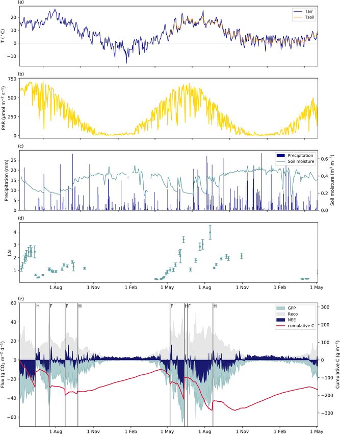
L. Heimsch et al.: CO2 fluxes and C balance of an agricultural grassland in southern Finland                               3469

annual air temperature and precipitation at the Kaarina Yltöi-    2018 to 3 May 2020. From this point on, the periods of 4
nen weather station, located 13 km northeast of Qvidja, were      May 2018–3 May 2019 and 4 May 2019–3 May 2020 are
5.4 ◦ C and 679 mm, respectively (Pirinen et al., 2012). The      referred to as the first and second EC measurement years,
experimental field in Qvidja has mineral soil (clay loam), and    respectively.
it covers 16.25 ha. It was cultivated as forage grassland dur-       The EC instrumentation consisted of an enclosed in-
ing the study years. From 2008 to 2016, the field was man-        frared gas analyser (LI-7200, LI-COR Biosciences, NE,
aged intensively with conventional practices, and it was in       USA), which detects the CO2 and H2 O mixing ratios, and
annual crop rotation. In 2017, the field management prac-         a three-dimensional sonic anemometer (uSonic-3 Scientific,
tices were converted towards more sustainable and environ-        METEK GmbH, Elmshorn, Germany) to measure wind
mentally friendly farming by increasing the use of organic        speed and air temperature. The data were recorded at 10 Hz
fertilizers and perennials, restricting the use of pesticides     frequency. The measurement height was 2.3 m. The flow rate
and increasing plant species biodiversity. The current grass      was about 12 L min−1 , and the length of the 4 mm stainless-
and clover mixture was sown as an undergrown species with         steel inlet tube with 2 µm Swagelok sinter was 0.8 m. The
broad bean in spring 2017. The predominant species were           CO2 measurements were regularly checked with zero and
timothy (Phleum pratense), meadow fescue (Festuca praten-         span gases, and the LI-7200 was recalibrated when neces-
sis) and white clover (Trifolium repens).                         sary. The H2 O measurements were compared with the data
   Grass was harvested for silage for the first time on 12 June   obtained from a dedicated humidity sensor; no recalibration
2018. As the grass cover was fairly sparse later in the summer    was necessary.
due to drought, oversowing was done on 3 September 2018              The micrometeorological sign convention is used through-
to restore the drought-induced damage. The seed mixture in-       out the paper, with a negative value indicating the flux from
cluded 35 % of timothy, 30 % of rye grasses (Lolium spp.),        the atmosphere to the ecosystem (net uptake) and a positive
20 % of common meadow grass (Poa pratensis) and 15 %              value indicating the flux from the ecosystem to the atmo-
of red fescue (Festuca rubra). Timothy, meadow fescue and         sphere (net emission).
clover remained as the predominant species in 2019 and early         Auxiliary meteorological measurements were conducted
2020. On 21 August 2018, the grass was cut at approximately       next to the flux tower. These included soil moisture observa-
15 cm, but the yield was left in the field. The second harvest    tions at the depth of 0.1 m (ML3 ThetaProbe sensor, Delta-
of 2018 occurred on 23 September. In 2019, the grass was          T Devices Ltd., Cambridge, UK) and soil temperature pro-
harvested on 11 June and 20 August. In June 2018, a conven-       files at the depths of 5, 10 and 30 cm (Pt100 IKES sensors,
tional cutting height of 6 cm was used, whereas in the other      Nokeval Oy, Nokia, Finland). The soil temperature data were
harvests the grass was cut at 15 cm.                              collected with a Vaisala QML201C datalogger (Vaisala Oyj,
   In 2018, the field was fertilized twice, on 16 July and 24     Vantaa, Finland). Photosynthetically active radiation (PQS
August, with 2800 and 1800 kg ha−1 of NK-molasses, re-            PAR sensor, Kipp & Zonen B.V., Delft, the Netherlands),
spectively (Table 1). NK-molasses is a byproduct of the sugar     global and reflected solar radiation (CMP3 radiometer, Kipp
industry. It contained 67 % of organic matter (OM) and 4.4 %      & Zonen), and air temperature and relative humidity (Hum-
of nitrogen and had the C : N ratio of 9. According to the        icap HMP155, Vaisala Oyj) were measured at the height of
product information, the molasses included 205 g kg−1 of or-      1.8 m. In addition, precipitation was measured with a weigh-
ganic carbon. In addition, it contained potassium and small       ing rain gauge (Pluvio2, OTT HydroMet GmbH, Kempten,
proportions of sulfur, magnesium, calcium and sodium.             Germany). Meteorological measurements started on 8 May
   In May 2019, the field was fertilized with a mixture of        2018, and the data were recorded as 30 min averages, ex-
side products from industries of starch potato processing,        cluding the precipitation which was recorded as 1 min values.
biowaste processing and ethanol production out of sawdust.        Snow depth was recorded at the weather station of Kaarina
This fertilization mixture contained 70 % (of dry weight) of      Yltöinen.
OM, 1.3 % of nitrogen, 0.2 % of phosphorus, 3 % of potas-            The leaf area index (LAI) data were obtained from the
sium and 0.4 % of sulfur, as well as small amounts of cal-        Sentinel-2 satellite as daily values on the clear-sky days. LAI
cium, magnesium, zinc, copper and manganese. Approxi-             was calculated from the Sentinel-2 bottom-of-atmosphere
mately 4600 kg ha−1 was applied to the field on 8 May (Ta-        products (L2A) using the Google Earth Engine (GEE) and
ble 1). On 26 June after the first harvest, 220 kg ha−1 of min-   a Python implementation of the Biophysical Processor tool-
eral fertilizers was applied. This fertilizer contained 23 % of   box (Weiss and Baret, 2016) available in Sentinel Applica-
nitrogen, 10 % of phosphorus and 8 % of potassium.                tion Platform (SNAP) software. The cloudy, cloud-shadowed
                                                                  and snowy data were filtered out using the scene classifica-
2.2   Measurement setup                                           tion band available in the L2A products.

The CO2 and H2 O fluxes were measured with the microme-
teorological EC method. The flux measurements started on 3
May 2018, and here we analysed data collected from 4 May

https://doi.org/10.5194/bg-18-3467-2021                                                  Biogeosciences, 18, 3467–3483, 2021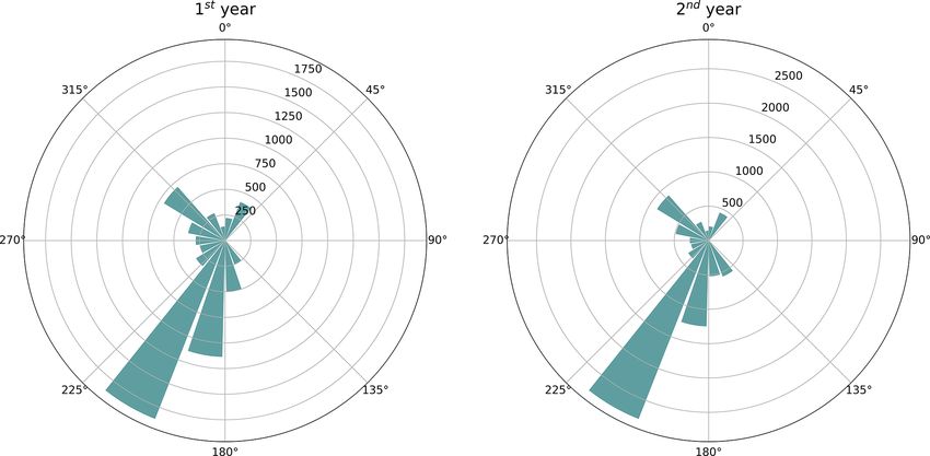
3470                          L. Heimsch et al.: CO2 fluxes and C balance of an agricultural grassland in southern Finland

Figure 1. Experimental field with the sectors representing the target area that covers 3.9 ha. Eddy covariance tower is located in the centre of
the sectors. EC data from wind directions from 30 to 140◦ were discarded due to another experimental plot located in that part of the field.
(Orthophoto from National Land Survey of Finland.)

Table 1. Different management events and their C inputs (fertilization) and C outputs (harvest). During the cutting in August 2018, the grass
was not collected and thus did not result in any C flux allocated to management.

                          Date             Management                              Output           Input    Carbon
                                                                     (dry weight kg ha−1 )     (kg ha−1 )   (g m−2 )
                          12 Jun 2018      Harvest                                    1985                       83
                          16 Jul 2018      Fertilization                                          −2800         −57
                          21 Aug 2018      Cutting                                        –           –           –
                          24 Aug 2018      Fertilization                                          −1755         −36
                          23 Sep 2018      Harvest                                     348                       15
                          8 May 2019       Fertilization                                          −4606         −43
                          11 Jun 2019      Harvest                                    3107                      130
                          20 Jun 2019      Fertilization (mineral)                       –             –          –
                          20 Aug 2019      Harvest                                    1029                       43

2.3    Eddy covariance data processing                                    this period, the 10 Hz mixing ratios were recalculated from
                                                                          the recorded absorptance data using the instrument-specific
                                                                          calibration functions. The mean CO2 mixing ratio was set to
The turbulent fluxes were determined as the covariance be-
                                                                          410 ppm in these calculations.
tween the variations in vertical wind component and gas mix-
                                                                             The following acceptance criteria were applied to screen
ing ratio recorded at 10 Hz. They were calculated as 30 min
                                                                          the 30 min averaged CO2 flux data: number of spikes in
block averages applying standard procedures, including dou-
                                                                          the raw data < 150 of 18 000, relative stationarity of CO2
ble coordinate rotation and lag determination based on cross-
                                                                          flux (Foken et al., 2012) < 50 %, mean CO2 mixing ratio
correlation analysis (Rebmann et al., 2012). The systematic
                                                                          > 380 ppm, variance of CO2 mixing ratio < 15 ppm2 be-
flux loss due to the incomplete frequency response of the
                                                                          tween April and September and < 5 ppm2 between October
measurement system was corrected according to the empiri-
                                                                          and March, and wind direction within 0–30◦ or 140–360◦ .
cal method described by Laurila et al. (2005).
                                                                          Furthermore, the data were discarded during the periods of
   The EC data from 5 January to 28 March 2019 were af-
                                                                          weak turbulence and when the flux footprint was not suf-
fected by technical issues with an inlet filter, which resulted
                                                                          ficiently representative of the target grassland, as estimated
in an erroneous reading of the internal analyser pressure. For

Biogeosciences, 18, 3467–3483, 2021                                                            https://doi.org/10.5194/bg-18-3467-2021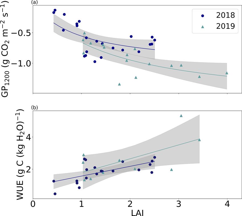
L. Heimsch et al.: CO2 fluxes and C balance of an agricultural grassland in southern Finland                                3471

with the footprint model of Kormann and Meixner (2001).           The carbon balance was calculated by adding up the 30 min
For these, we applied a friction velocity limit of 0.06 m s−1     NEE fluxes, the imported carbon in the form of organic fer-
and a cumulative footprint limit of 0.7. The further screening    tilizers and the carbon removed as harvested biomass:
applied to H2 O fluxes included H2 O flux > 0, relative sta-                             n
tionarity of H2 O flux < 50 % and variance of H2 O mixing
                                                                                         X
                                                                  Cbalance = CH + CF +         NEEi ,                         (4)
ratio < 1 (mmol mol−1 )2 . After applying these filtering cri-                           i=1
teria, the coverage of CO2 and H2 O flux data accepted for
further analysis was 44 % and 30 % of all the 30 min periods      where CH is the amount of carbon in harvested biomass,
(i.e. total of 35 088 time steps) during the 2 measurement        CF is the amount of carbon in imported fertilization and n
years, respectively (for CO2 , day/night 55 %/33 %, April–        is the total number of time steps in the period for which
September/October–March 48 %/38 %; for H2 O, day/night            the balance was calculated. Thus, the carbon balance indi-
49 %/11 %, April–September/October–March 41 %/16 %).              cates the net ecosystem carbon balance as defined by Chapin
Most of the accepted CO2 and H2 O flux data were collected        et al. (2006) without the contribution of carbon monox-
when the wind direction was in the south-southwest sector         ide, methane, volatile organic and particulate compounds,
(Fig. 2).                                                         or leaching. This balance is commonly called the net biome
                                                                  production (Kutsch et al., 2010). Biomass was converted to
2.4   Flux partitioning and gap-filling                           carbon by multiplying the dry weight by 0.42 (Lohila et al.,
                                                                  2004). The following sign convention was used: the carbon
To calculate CO2 balances and to analyse the components of        imported into the ecosystem corresponds to a negative flux,
the net ecosystem exchange between the field and the atmo-        and the carbon removed from the system corresponds to a
sphere, the measured CO2 flux data (i.e. net ecosystem ex-        positive flux.
change, NEE) were partitioned to GPP and total ecosystem
respiration (Reco ) and gap-filled based on this partitioning:    2.6   Uncertainty analysis
NEE = GPP + Reco .                                         (1)    The CO2 balance between the field and the atmosphere,
The gap-filled GPP and Reco were calculated with empirical        which is calculated based on the EC measurements, includes
response functions by first fitting these functions to the flux   multiple potential error sources. Uncertainties are associated,
data. Reco was expressed as a function of temperature (Lloyd      for example, with the stochastic nature of turbulence and in-
and Taylor, 1994):                                                complete sampling of large eddies, the performance of in-
                                                                struments and the flux variation caused by the limited area
                        1      1
              E0       T1 − Ta −T0                                of the target ecosystem (Aubinet et al., 2012). The most rel-
Reco = R0 e                              ,                 (2)
                                                                  evant random error sources, i.e. the statistical measurement
where R0 is the respiration rate (mg m−2 s−1 ) at the refer-      error (Emeas ) and the error caused by gap-filling (Egap ) (Au-
ence temperature of 283.15 K, T0 = 227.13 K, T1 = 56.02 K,        rela et al., 2002), were included in the uncertainty estimate:
E0 is ecosystem sensitivity coefficient (Lloyd and Taylor,                  v
1994) that describes the temperature response of soil respira-              u n
                                                                            uX
tion and Ta is the air temperature.                               Emeas = t (NEEmeas,i − NEEmod,i )2 ,                         (5)
   GPP was modelled as a function of photosynthetically ac-                   i=1
tive radiation (PAR, µmol m−2 s−1 ) as
                                                                  where NEEmeas is the filtered 30 min flux, NEEmod is the cor-
        α × PAR × GPmax                                           responding modelled NEE (Eqs. 1–3) and n is the number of
GPP =                   ,                                  (3)
        α × PAR + GPmax                                           measured data.
where α is the apparent quantum yield (mg µmol−1 ), and                  v
                                                                         uN
GPmax denotes the asymptotic CO2 uptake rate in optimal                  uX
                                                                                 2
                                                                  Egap = t (EGPP,i     + ER2 eco ,i ),                      (6)
light conditions (mg m−2 s−1 ). Further details on the gap-                  i=1
filling procedure are provided in Appendix A. Energy fluxes
were gap-filled following the description in Appendix B.          where EGPP and EReco are the errors of modelled GPP and
    To study the differences in photosynthetic capacity of the    Reco , respectively. N is the number of gaps in the data.
grass field between the two growing seasons, daily GP1200           The standard error propagation principle was used in esti-
values were calculated with the estimated α and GPmax val-        mating the total uncertainty (Etot ) of the annual carbon bal-
ues; i.e. GPP was normalized to PAR = 1200 µmol m−2 s−1 .         ance:
                                                                          q
2.5   Net ecosystem carbon balance                                Etot = Emeas2        2 .
                                                                                   + Egap                                    (7)
In this study, the system boundaries include the main com-
ponents of the carbon balance of the field ecosystem studied.

https://doi.org/10.5194/bg-18-3467-2021                                                  Biogeosciences, 18, 3467–3483, 2021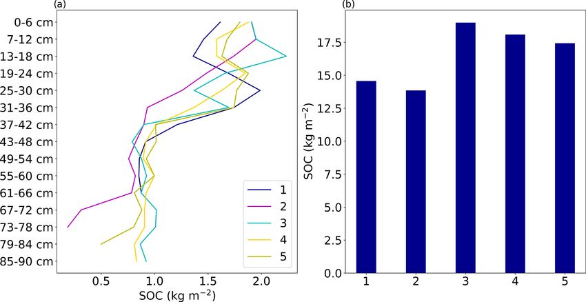
3472                          L. Heimsch et al.: CO2 fluxes and C balance of an agricultural grassland in southern Finland

Figure 2. Number of accepted flux measurements within 20◦ sectors around the flux tower during the first and second years. Data from 30
to 140◦ were discarded.

2.7    Water use efficiency                                           5 ◦ C, started on 14 April in 2018, i.e. before the EC mea-
                                                                      surements started. In 2019 and 2020, the thermal growing
The ecosystem WUE was defined as the ratio of GPP to ET,              season began on 16 and 18 April, respectively. The thermal
i.e. H2 O flux:                                                       growing season ended on 17 November and 26 October in
          GPP                                                         2018 and 2019, respectively. Thus, the thermal growing sea-
WUE =         ,                                           (8)         son length was 218 d in 2018 and 194 d in 2019. Meteoro-
          ET
                                                                      logical conditions during the main growing season between
where daily means of GPP and ET were used. The ET data
                                                                      May and September varied substantially between the 2 years.
corresponding to a latent heat flux lower than 30 W m−2 were
                                                                      The mean air temperature during these periods was 16.7 and
discarded (Abraha et al., 2016). Furthermore, days with pre-
                                                                      14.5 ◦ C in 2018 and 2019, respectively. During the same pe-
cipitation were eliminated in order to obtain a signal that is
                                                                      riod, the mean daily PAR was about 12 % higher in 2018 than
dominated by transpiration.
                                                                      in 2019 (460 vs. 410 µmol m−2 s−1 ), while the precipitation
2.8    Soil carbon storage                                            sum was 32 % lower (212 vs. 312 mm).
                                                                         During winter 2018–2019, permanent snow cover was
Soil carbon content was determined from 1 m deep core sam-            recorded from 17 December 2018 to 26 March 2019. In the
ples taken within the flux source area. The samples were              following winter (2019–2020), there were only two short
taken in October 2018 using a hydraulic corer installed on            snow-cover periods: 5–8 February and 30–31 March 2020.
a tractor. The diameter of the sample cylinder was 151 mm.            The maximum snow depth in the first winter was 33 cm,
Subsamples were taken along the 1 m core at 16 points, and            whereas in the second winter it was 3 cm. The mean win-
soil organic carbon (SOC, kg m−2 ) content in each subsam-            tertime (November–March) air temperature was −0.2 ◦ C in
ple was analysed using a VarioMax CN analyser (Elementar              2018–2019 and 2.2 ◦ C in 2019–2020.
Analysensysteme GmbH, Germany).                                          Soil moisture content at the depth of 10 cm varied between
                                                                      0.16 and 0.55 m3 m−3 during the study period. On several
                                                                      occasions, the daily mean soil moisture dropped to about
3     Results                                                         0.2 m3 m−3 . During the growing seasons, such low values
                                                                      indicate substantial drought, while in the winter, rapid data
3.1    Meteorological conditions                                      drops were likely related to soil freezing. The average soil
                                                                      moisture during the growing season in 2019 was higher than
The annual mean air temperature at the study site was 7.6
                                                                      in 2018 (0.30 vs. 0.26 m3 m−3 ). As a result of the higher pre-
and 7.7 ◦ C in the first and second measurement years, re-
                                                                      cipitation in 2019, soil moisture occasionally increased up
spectively. Both years were warm compared to the long-term
                                                                      to 0.4 m3 m−3 , i.e. close to the saturated values observed in
(1981–2010) average of 5.4 ◦ C measured at a nearby weather
                                                                      winter.
station (Pirinen et al., 2012). The annual precipitation sum
was lower in the first year (473 mm) and higher in the second
year (855 mm) than the long-time average (679 mm).
   The thermal growing season, defined here as the period
when the daily mean temperature permanently exceeded

Biogeosciences, 18, 3467–3483, 2021                                                      https://doi.org/10.5194/bg-18-3467-2021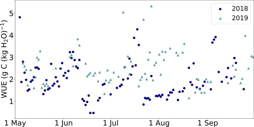
L. Heimsch et al.: CO2 fluxes and C balance of an agricultural grassland in southern Finland                                3473

3.2   CO2 and H2 O fluxes                                         after the fertilizations in July 2018 and May 2019, poten-
                                                                  tially affecting CO2 fluxes. After the fertilization events with
At the beginning of the measurements, the net CO2 fluxes          organic substances in July 2018, August 2018 and May 2019,
were negative (Fig. 3), and the air temperature was al-           the mean PAR was 7 %, 29 % and 12 % lower, respectively,
ready well above 10 ◦ C (Fig. 4). Net uptake was ob-              than the 5 d mean before the fertilization, complicating the
served until the first harvest around mid-June 2018. This         interpretation of fertilization impacts on the CO2 fluxes. The
harvest and the following management events during that           effect of management on H2 O fluxes could not be disentan-
growing season induced large short-term variations in the         gled from the present data (Fig. 3b).
CO2 fluxes. Similarly, in the second study year, large im-           The LAI derived from Sentinel-2 images (Fig. 4d) var-
pacts on CO2 fluxes were observed after the management            ied greatly between the years. The higher LAI in 2019 indi-
events. During the growing season, the mean NEE was               cated that there was more photosynthesizing green biomass
−0.13 and −0.21 mg CO2 m−2 s−1 in 2018 and 2019, re-              before the first and second harvests compared to 2018. The
spectively. During the wintertime, no significant CO2 up-         effect of larger leaf area was also observed in the differences
take occurred, and the positive fluxes were small com-            in the photosynthetic capacity (GP1200 ) of the grassland be-
pared to the nocturnal fluxes in summer. The mean mea-            tween the study years (Fig. 5a). The years differed signif-
sured NEE between December 2018 and February 2019 was             icantly (p < 0.05) in terms of GP1200 at all levels of LAI
0.03 mg CO2 m−2 s−1 , and during the same period in 2019–         (> 1). Larger LAI values were observed throughout 2019, in-
2020 it was 0.04 mg CO2 m−2 s−1 .                                 dicating that grass was growing better than in 2018. Further-
   Seasonal patterns were also observed in the H2 O fluxes        more, the grassland was photosynthesizing more efficiently
(Fig. 3). In the spring, the ecosystem ET started to in-          with the same leaf area in 2019 than in the previous year
crease, reaching the highest levels between June and Au-          (Fig. 5a).
gust, after which it gradually decreased to wintertime values,
i.e. close to zero. The mean growing season H2 O flux was         3.3   Water use efficiency
34.7 mg H2 O m−2 s−1 in 2018 and 35.5 mg H2 O m−2 s−1 in
2019. The wintertime (December–February) mean H2 O flux           The ecosystem WUE estimate showed different seasonal
was 3.6 and 3.7 mg H2 O m−2 in 2018–2019 and 2019–2020,           variation during the studied growing seasons (Fig. 6). Gen-
respectively.                                                     erally, WUE was higher in 2019 than in 2018 throughout
   The experimental field was harvested and fertilized twice      the growing season. WUE increased before the first har-
during each of the studied growing seasons (Table 1).             vest around mid-June in both years, indicating more effi-
The effect of management was investigated by compar-              cient CO2 uptake in terms of water use than during the
ing the mean fluxes 5 d before and after the harvest dates        spring. The 5 d mean WUE before the first harvest was 2.8
(Table C1). The harvest in June 2018 changed the mean             and 3.0 g CO2 (kg H2 O)−1 in 2018 and 2019, respectively.
CO2 flux from a net sink of −0.28 mg CO2 m−2 s−1 to a             Due to the harvest, it dropped to 0.9 g CO2 (kg H2 O)−1 in
source of 0.03 mg CO2 m−2 s−1 , i.e. increased the net ef-        2018 and to 2.6 g CO2 (kg H2 O)−1 in 2019. During the lat-
flux by 0.31 mg CO2 m−2 s−1 . The first harvest of 2019           ter growing season, WUE increased steadily towards 4 g CO2
increased NEE by 0.47 mg CO2 m−2 s−1 , but as the pre-            (kg H2 O)−1 until the second harvest in August, whereas in
harvest mean NEE was −0.50 mg CO2 m−2 s−1 , the field             2018 it remained predominantly below 2 g CO2 (kg H2 O)−1
remained as a net sink. As a result of the second har-            during the same period. At the end of August and early
vest on 23 September 2018, the mean sink decreased from           September, WUE was at the same level in both years.
−0.10 to −0.02 mg CO2 m−2 s−1 , while the harvest on 20              The LAI derived from the Sentinel-2 data was compared to
August 2019 caused the sink to change from −0.25 to               the daily WUE values (Fig. 5b) to further cast light on the re-
−0.02 mg CO2 m−2 s−1 . Thus, after all the harvests with a        lationship between vegetation status and WUE. While WUE
cutting height of 15 cm, the mean sink rate was diminished        was on average lower in 2018 than 2019, the difference at a
to −0.02 or −0.03 mg CO2 m−2 s−1 .                                given LAI was not significant (p > 0.05). However, in both
   In the first growing season, the first and second fertiliza-   years the daily WUE increased in a similarly linear manner
tion events with organic substances increased NEE by 0.27         in relation to LAI.
and 0.08 mg CO2 m−2 s−1 , respectively, i.e. diminished the
CO2 sink (Fig. 3, Table C1). During the 5 d after the har-        3.4   Carbon balance and soil carbon storage
vest in May 2019, the field acted as a CO2 source. A similar
trend was not observed in June 2019, as mineral fertilizer was    The carbon balance of the studied grass field was
used, and thus no organic substances were added to the soil.      −57 ± 10 g C m−2 yr−1 in the first year, and the balance of
Each of the fertilization events were followed by rain within     the second year was −86 ± 12 g C m−2 yr−1 , i.e. the field
the next 5 d. However, the mean soil moisture at the depth of     acted as a net carbon sink in both years (Table 2). The mag-
10 cm either remained the same or decreased slightly (Fig. 4,     nitude of all components of the carbon balance were smaller
Table C1). Furthermore, the mean air temperature increased        in the first year than in the second one, GPP by 29 %, Reco

https://doi.org/10.5194/bg-18-3467-2021                                                  Biogeosciences, 18, 3467–3483, 2021
3474 L. Heimsch et al.: CO2 fluxes and C balance of an agricultural grassland in southern Finland
Figure 3. Accepted 30 min (a) net ecosystem exchange (NEE) and (b) H2 O flux measurements from May 2018 to May 2020. Vertical lines
with H and F indicate harvest and fertilization, respectively.
Table 2. The annual carbon balances and their components that the magnitude of the net carbon balance represented the
(g C m−2 yr−1 ) for the 2 measurement years. Negative values in- amount of carbon accumulated in the soil. Furthermore, to
dicate C input into the ecosystem, whereas positive values indicate evaluate whether the field had the potential to fulfil the “4
C loss. Management (M) is the sum of the C fluxes due to harvest per 1000” initiative, the annual net carbon balance was com-
(positive) and fertilization (negative) events (Table 1). The values pared to the average soil carbon content. Thus, the estimated
after ± represent the uncertainty in NEE.
increase in soil carbon storage was 0.3 % and 0.5 % in the
first and second years, respectively. On average, the annual
NEE GPP Reco M Total balance
carbon input to the soil accounted for 0.4 % of the SOC.
First year −62 −1121 1053 5 −57 ± 10
Second year −216 −1583 1362 130 −86 ± 12
4 Discussion
Table 3. Net ecosystem exchange of CO2 (NEE, g CO2 m−2 ), its
4.1 Fluxes and carbon balance
components gross primary production (GPP) and ecosystem respi-
ration (Reco ), and evapotranspiration (ET, mm) during the growing
season (4 May to 30 September) in 2018 and 2019.
There is an urgent need to find evidence-based climate-
friendly practices in agriculture in the boreal region, where
Year NEE GPP Reco ET the growing season is short and varieties differ from
those cultivated in the temperate region. The carbon fluxes
2018 −601 −3330 2715 297 we measured on the agricultural grassland at the Qvidja
2019 −1176 −4955 3771 283 farm in southern Finland clearly indicated that this site
was a sink of atmospheric carbon. The annual NEE was
−62 g C m−2 yr−1 in the first study year (4 May 2018–3 May
by 23 % and management by 96 %. The components in the 2019) and −216 g C m−2 yr−1 in the second year (4 May
mean annual CO2 fluxes between the field and the atmo- 2019–3 May 2020). The GPP showed notable variation be-
sphere also indicated major differences between the growing tween the study years as the annual GPP was −1121 and
seasons (Table 3). In 2019, the magnitude of the growing sea- −1583 g C m−2 yr−1 in the first and second years, respec-
son NEE was 78 %, GPP 49 % and Reco 42 % higher than in tively. Gilmanov et al. (2010) reported a range of −2107
2018. to −1410 g C m−2 yr−1 for the GPP of European managed
The average soil carbon storage in the 1 m layer was grasslands. Our results fall below or in the lower end of this
16.59 ± 2.25 kg m−2 (average ± standard deviation), with range. The annual Reco in Qvidja also varied between the
the highest SOC found in the top 30 cm layer (Fig. 7). To study years (1053 and 1362 g C m−2 yr−1 ). The annual Reco
estimate the increase in soil carbon storage, it was assumed in the European grasslands is reported to vary between 494
Biogeosciences, 18, 3467–3483, 2021 https://doi.org/10.5194/bg-18-3467-2021L. Heimsch et al.: CO2 fluxes and C balance of an agricultural grassland in southern Finland 3475 Figure 4. Daily mean (a) air and soil (depth = 0.05 m) temperature, (b) photosynthetically active radiation (PAR), (c) precipitation and soil moisture (depth = 0.1 m), (d) leaf area index (LAI), and (e) daily mean NEE, GPP, Reco and cumulative carbon flux from May 2018 to May 2020. https://doi.org/10.5194/bg-18-3467-2021 Biogeosciences, 18, 3467–3483, 2021
3476                         L. Heimsch et al.: CO2 fluxes and C balance of an agricultural grassland in southern Finland

                                                                      source. Mineral fertilizers were used during their study, and
                                                                      thereby no carbon was imported to the field to compensate
                                                                      for the biomass removal from the system as harvests. Simi-
                                                                      lar management-related carbon flux patterns were observed
                                                                      by Eichelmann et al. (2016), who reported a more negative
                                                                      NEE (average −405 g C m−2 yr−1 ) for an agricultural grass-
                                                                      land in Canada than the NEE in Qvidja; however, the 2-year
                                                                      mean annual carbon balance was positive when biomass re-
                                                                      moval was taken into account, i.e. the Canadian field was a
                                                                      net source of carbon. It is noteworthy that the yield in Qvidja
                                                                      was substantially smaller than at the other two study sites
                                                                      (Lind et al., 2016; Eichelmann et al., 2016), at which the to-
                                                                      tal balance became positive when the management activities,
                                                                      i.e. harvests and fertilization, were taken into account. The
                                                                      total carbon balance of the field depends greatly both on the
                                                                      amount of organic matter imported to the system as fertiliz-
                                                                      ers and on the harvest yields, which are affected, for instance,
                                                                      by the applied cutting height.
Figure 5. (a) Daily photosynthetic capacity (GP1200 ) and (b) water      Analysis of the weather variables in Qvidja indicated that
use efficiency (WUE) as a function of leaf area index (LAI) dur-      temperature and moisture conditions were associated with
ing the two growing seasons. Grey areas represent the uncertainty     the differences in CO2 flux dynamics and carbon balance be-
bands.                                                                tween the study years. The growing season was warmer and
                                                                      drier in 2018 than 2019, with 13 % lower mean soil mois-
                                                                      ture, 32 % lower precipitation, 2.2 ◦ C higher mean air tem-
                                                                      perature and 12 % higher mean radiation during the growing
                                                                      season, and substantially smaller fluxes were observed in the
                                                                      first year. This is in accordance with Shurpali et al. (2009),
                                                                      who observed a positive correlation between the uptake of
                                                                      atmospheric CO2 (GPP) and both soil moisture and air tem-
                                                                      perature on another Finnish agricultural grassland. Accord-
                                                                      ing to their conclusions, moderate temperature with high soil
                                                                      moisture enhanced CO2 uptake. Furthermore, Flanagan et al.
                                                                      (2002) and Kurc and Small (2007) concluded that rather wet
                                                                      summer conditions favoured photosynthetic activity in grass-
Figure 6. Daily water use efficiency (WUE) during two growing         lands. These findings would support the conclusion that low
seasons.                                                              soil moisture and high temperatures were the main factors
                                                                      limiting CO2 uptake at our study site in the summer 2018.
                                                                      However, this question remains partly open, as weather con-
and 1623 g C m−2 yr−1 (Gilmanov et al., 2007). Our obser-             ditions, grass age and grass leaf area all showed different
vations are thus also within this range.                              dynamics between the study years. In Finland, it is typical
   To answer our first research question, we concluded                to grow grasslands for 3–4 years before grass renewal. In
that the carbon balance was negative in both study years              Qvidja, the grass was not renewed between the study years,
(−57 ± 10 and −86 ± 12 g C m−2 yr−1 ), and thus the field             which may have led to the larger fluxes observed in the sec-
acted as a net carbon sink during the study period. In com-           ond year when the grass root system, for instance, was likely
parison, the Finnish agricultural fields measured so far were         to be more developed, enhancing water and nutrient avail-
generally carbon sources when ecosystem–atmosphere CO2                ability and thus reducing the effect of drought stress. Further-
fluxes, harvests and the carbon supplied to the system as             more, the leaf area was larger, and other capabilities, such as
fertilizers were considered (Heikkinen et al., 2013; Shurpali         microbial symbioses (e.g. de Vries et al., 2020; Harman and
et al., 2009; Lind et al., 2016; Lohila et al., 2004). Lind et al.    Uphoff, 2019; Moreau et al., 2019), of the more developed
(2016) reported a slightly more negative annual NEE (2-               grass may have increased carbon uptake. The lower leaf area
year average NEE −259 g C m−2 yr−1 ) for a grassland site on          during the first year was most probably also due to the dry
mineral soil than we observed in Qvidja. However, by con-             summer, as shortage of water is a growth-limiting factor. Be-
sidering the total carbon balance of the system by taking into        sides the leaf area, the photosynthetic potential per leaf area
account the carbon fluxes related to biomass removal as grass         was lower in the first year, indicating either drought stress or
yield, it was concluded that their site acted as a net carbon         shortage of nutrients, as temperature, a widely limiting factor

Biogeosciences, 18, 3467–3483, 2021                                                      https://doi.org/10.5194/bg-18-3467-2021
L. Heimsch et al.: CO2 fluxes and C balance of an agricultural grassland in southern Finland 3477
Figure 7. (a) Soil organic carbon (SOC) content at different depths in the 1 m deep soil samples, and (b) the total SOC in the samples.
Numbers from 1 to 5 indicate sample numbers.
in northern latitudes, was high enough during both summers served on northern grasslands (0–7 g C (kg H2 O)−1 ) (Tang
not to restrict photosynthesis. In any case, a more specific et al., 2014).
analysis of the driving and inhibiting environmental factors The different management practices, such as fertilization
will require a longer measurement period. and the choice of grass cutting height, were slightly different
Our second research question concerned the drought- in the first and second years, which probably had an impact
related restrictions of photosynthesis. It has been widely rec- on the carbon balances. In June 2018, a conventional cut-
ognized that in dry conditions plants are able to reduce tran- ting height of 6 cm was used, whereas in the other harvests
spiration by stomatal regulation (Willmer and Fricker, 1996). the grass was cut at 15 cm. The higher cutting height may
However, grasses seem to limit stomatal functions only in have enhanced the regrowth of grass, especially in the more
severe, prolonged drought conditions (Wolf et al., 2013; Xu favourable weather conditions in 2019, and with a larger leaf
et al., 2019), and thus occasional or seasonal drought events area higher CO2 uptake was observed right after the harvest.
may not be observed in the ecosystem WUE of grasslands. Only after the 6 cm harvest did the field turn to a net source
In our study, WUE values were predominantly lower in 2018 of CO2 . With a low cutting height, it was more likely that the
than in 2019. This was most probably explained by the dif- grass was cut below the growing point, particularly in dry
ferences in LAI, as the relationship between WUE and LAI conditions, which affects the stand longevity and stress tol-
was similar during both growing seasons (Fig. 5b). Further- erance (Jones and Tracy, 2018). As the weather was warm
more, the drier conditions with high temperatures in the sum- and dry during the harvest events in June in both years, a
mer 2018 may have resulted in a decoupling of assimilation higher cutting height may have served as a vital management
and transpiration and in temperature-induced downregula- improvement.
tion of GPP (Gharun et al., 2020), as ET was similar in both The field was mainly fertilized with organic substances,
years (Table 3). Therefore, the clearly lower leaf-area-based and thus carbon was imported to the system, affecting the net
photosynthetic capacity (GP1200 ) in 2018 compared to 2019 carbon balance. After each of the fertilization events with or-
probably indicates drought-related stress on photosynthetic ganic material, the respiration of the field increased, whereas
processes despite the similar leaf-area-based WUE (Fig. 5). mineral fertilization was not observed to have an immedi-
It is noteworthy that the WUE analysis was performed by ate effect on CO2 fluxes. Increased respiration was likely
means of the total ecosystem ET rather than plant transpira- to occur due to microbial activity of the organic fertilizers.
tion, which would have enabled a more direct determination Gilmanov et al. (2007) observed on a Danish agricultural
of the actual plant WUE and thus a simpler interpretation grassland that, although the application of manure increased
of plant processes and their relation to LAI. Nevertheless, respiration, the plant uptake of CO2 was notably higher than
days with even slight precipitation were eliminated from the at the other sites studied. Fornara et al. (2016) also con-
analysis, and therefore we can assume that during the grow- cluded, based on their 43-year study, that manure fertilization
ing season most of the water flux arises from transpiration. substantially increased soil carbon sequestration of a grass-
In general, WUE at our study site varied mainly between 0 land ecosystem in Northern Ireland. Although the type of the
and 4 g C (kg H2 O)−1 . This is consistent with the WUEs ob- organic fertilizer possibly plays a crucial role, the applica-
tion of carbon to the system has a direct effect on the carbon
https://doi.org/10.5194/bg-18-3467-2021 Biogeosciences, 18, 3467–3483, 20213478 L. Heimsch et al.: CO2 fluxes and C balance of an agricultural grassland in southern Finland
balance, but there is also an indirect effect on its components mainly driven by meteorological and hydrological conditions
Reco and GPP via soil and plant functions. (Manninen et al., 2018), but it is also affected by soil proper-
Concerning our final research question on the relation of ties (Don and Schulze, 2008). Large variations in soil mois-
the carbon balance to the international “4 per 1000” car- ture and temperature and precipitation may increase the sol-
bon sequestration initiative (Minasny et al., 2017), our re- ubility of SOM. Generally, however, clay soils retain carbon
sults show that the Qvidja field acted as an annual net car- better than other soil types. Furthermore, ploughing increases
bon sink and had the potential to fulfil the goal of this ini- leaching as mineralization of SOM is enhanced. Depending
tiative and to contribute to the short-term climate change on precipitation and hydrological and chemical properties of
mitigation. By considering the carbon balance by account- the soil, carbon leaching on grasslands may equal approxi-
ing for the ecosystem–atmosphere CO2 fluxes and the car- mately 25 % of the annual carbon balance calculated based
bon fluxes caused by management activities and comparing on NEE, harvest and fertilization (Kindler et al., 2011). At
that to the measured soil carbon content, the carbon storage our study site, the effect of leaching on the annual carbon
of the field increased on average by 0.4 % annually over the balance could be assumed to be fairly small in both sum-
studied period. To draw a more reliable conclusion about the mers due to low soil moisture and low precipitation. In win-
carbon sequestration, leaching and other carbon-containing ter, the leaching may have caused a temporary contribution
compounds must also be considered in further studies about to the carbon balance during wet periods and thus reduced
the carbon balance. Furthermore, the number of soil carbon the increase in soil carbon storage. For a more accurate car-
samples should be increased for a more accurate evalua- bon balance estimate of this site, however, the contribution of
tion of the soil carbon storage of the field, even though the leaching and all carbon-containing gases (e.g. CH4 ) should
variation among the present samples was small. However, be measured and the number of soil carbon storage measure-
the estimated annual carbon balance of our second study ments increased.
year (−86 g C m−2 yr−1 ) with improved management prac-
tices was within the range of annual carbon sequestration
potential (80–120 g C m−2 yr−1 ) that is evaluated to be at- 5 Conclusions
tainable with improved management practices (Lal, 2016).
The agricultural grassland site located at Qvidja in south-
Thus, this study demonstrates the potential for a positive im-
ern Finland acted as a net carbon sink during the 2 years
pact of northern agricultural grasslands in terms of climate
studied. The carbon balance of the first study year was
change mitigation.
−57 ± 10 g C m−2 yr−1 , and in the second year it was
−86 ± 12 g C m−2 yr−1 . When CO2 fluxes and carbon fluxes
4.2 Errors and uncertainties
caused by management activities were solely accounted for,
the soil carbon storage was assumed to have increased by
Uncertainties in the results are mainly related to the gaps in
0.3 % and 0.5 % in 2018 and 2019, respectively, indicating
the measurement data, which required gap-filling of miss-
that northern agricultural grasslands have a potential to con-
ing measurements with modelled data. The length of a gap
tribute to climate change mitigation. The data and results
increases the related uncertainty, but in our data there were
presented here act as a basis for the future studies that fo-
only three longer gaps (4, 8 and 9 d), which all occurred dur-
cus on the conversion of this farm from intensive agricul-
ing the first winter, when temperatures were low and only
tural practices towards more sustainable agricultural man-
minor fluxes could have been observed. All the other gaps
agement, especially on the impacts of such a conversion
were shorter than 3 d. However, each gap contributed to the
on the GHG fluxes occurring on mineral soils in northern
uncertainty and were included in the carbon balance calcula-
conditions. Even though we could quantify the sink capac-
tions. Further uncertainties, which were not included in the
ity of the field, further research with longer-term measure-
error estimates, were involved in the yield measurements and
ments is needed to evaluate the persistence of carbon seques-
fertilization input estimates, as well as in the fairly scarce
tration and storage, and wider measurements of carbon bal-
sample size of the soil carbon content measurements.
ance components were to be included. Longer time series and
Carbon balance was calculated based on the ecosystem–
broader GHG flux measurements are also essential to more
atmosphere CO2 fluxes and the inputs and outputs of harvest
closely study the causes of the interannual variation in GHG
and fertilization. Thus, no other gaseous carbon compounds,
fluxes and carbon and water balances at this site, for which
such as methane, were considered. Regina et al. (2007) re-
the present study provides a baseline.
ported that the annual methane balances of a Finnish clay soil
for 2 years were −0.009 and 0.034 g CH4 m−2 yr−1 . Based
on this estimate, the possible carbon emission as methane
accounts for less than 1 % of our annual carbon balance.
Leaching of dissolved carbon and emissions of volatile or-
ganic compounds may have had an effect on the annual car-
bon balance. Leaching of carbon from the agricultural soils is
Biogeosciences, 18, 3467–3483, 2021 https://doi.org/10.5194/bg-18-3467-2021L. Heimsch et al.: CO2 fluxes and C balance of an agricultural grassland in southern Finland 3479
Appendix A: Gap-filling of CO2 fluxes
The flux data set was separated into sections at the harvest
Soil moisture (m3 m−3 )
After
0.23
0.21
0.23
0.24
0.34
0.29
0.20
0.20
0.36
dates, and gap-filling was done separately for these sections
by first parameterizing and calculating Reco and then GPP.
The parameter R0 was determined for each day from the
nighttime data (PAR < 20 µmol m−2 s−1 ) with a 7 d moving
window. E0 was determined within the same moving win-
Before
0.24
0.23
NA
0.24
0.36
0.37
0.23
0.20
0.35
dow as R0 . If there were fewer than 24 measurements within
the time window, its length was increased by 1 d at both the
beginning and end until enough data were obtained. R0 was
Precipitation (mm)
After
0
8.3
1.2
10.4
8.6
3.7
0.7
2.5
9.9
allowed to vary between 0.001 and 1 mg m−2 s−1 . The same
minimum number of observations within a 3 d moving win-
Table C1. Mean flux and meteorological conditions 5 d before and after management. The management day is not included. NA: not available.
dow was used for determining α and GPmax from the ob-
served NEE from which the estimated Reco had been sub-
Before
0
0
0
6.7
0.7
1.5
0.4
0
12.6
tracted. α and GPmax were allowed to vary between −0.5 and
−0.00001 mg µmol−1 and −5.0 and −0.00001 mg m−2 s−1 ,
respectively.
After
16.4
22.4
17.2
14.5
8.6
9.6
15.8
17.0
15.9
Air T (◦ C)
Appendix B: Gap-filling of energy fluxes
Before
12.5
19.9
NA
15.7
15.1
3.2
21.2
17.5
16.0
The gaps in the net radiation (Rn ) time series were filled with
the monthly mean diurnal cycles. Soil heat flux (G) was not
PAR (µmol m−2 s−1 )
After
646
480
290
273
226
324
412
622
354
measured at our site, so it was estimated from the energy
balance closure during the periods when the other energy
fluxes were known. Gap-filling of G was done by assum-
ing a constant ratio between G and Rn (Liebethal and Fo-
ken, 2007). The ratio of 0.24 was calculated with linear re-
Before
563
516
NA
382
183
367
627
601
268
gression from the daytime data (between 10:00–15:00 local
time, UTC+2). The sensible and latent heat fluxes (QH and
QE , respectively) were gap-filled based on the procedure de-
WUE (g C kg−1 H2 O)
After
0.9
2.5
1.9
1.5
1.4
2.0
2.6
2.1
1.4
scribed by Kowalski et al. (2003). The gaps in the daytime
QH (Rn > 0) were filled with monthly linear regression with
Rn . The nighttime gaps in QH (Rn < 0) were filled with the
corresponding Rn values. The gaps in the daytime QE were
Before
2.8
2.4
NA
2.0
2.5
2.4
3.0
2.3
filled in such a way that the monthly mean energy balance 3.0
closure was achieved. The nighttime gaps in QE were set to
0.
NEE (mg CO2 m−2 s−1 )
After
0.03
0
–0.02
–0.02
–0.02
0.17
–0.03
–0.08
–0.02
Appendix C: Management effect on fluxes
The immediate effect of management on the measured NEE
and WUE was investigated by comparing the mean values of
Before
–0.28
–0.27
NA
–0.10
–0.10
–0.17
–0.50
–0.08
–0.25
5 d before and after the management day (Table C1).
Fertilization 24 Aug 2018
Fertilization 20 Jun 2019
Fertilization 8 May 2019
Fertilization 16 Jul 2018
Harvest 20 Aug 2019
Cutting 21 Aug 2018
Harvest 23 Sep 2018
Harvest 12 Jun 2018
Harvest 11 Jun 2019
https://doi.org/10.5194/bg-18-3467-2021 Biogeosciences, 18, 3467–3483, 20213480 L. Heimsch et al.: CO2 fluxes and C balance of an agricultural grassland in southern Finland
Data availability. The flux and meteorological data as well as past, present and future, Global Change Biol., 9, 479–492,
the SOC measurements and LAI data are available at Zen- https://doi.org/10.1046/j.1365-2486.2003.00629.x, 2003.
odo (https://doi.org/10.5281/zenodo.4647078, Heimsch et al., Bastos, A., Ciais, P., Friedlingstein, P., Sitch, S., Pongratz, J., Fan,
2020). L., Wigneron, J., Weber, U., Reichstein, M., Fu, Z., Anthoni,
P., Arneth, A., Haverd, V., Jain, A. K., Joetzjer, E., Knauer, J.,
Lienert, S., Loughran, T., McGuire, P. C., Tian, H., Viovy, N., and
Author contributions. JL and TL planned the flux measurements Zaehle, S.: Direct and seasonal legacy effects of the 2018 heat
and TL was responsible for the setup. JPT made the post-processing wave and drought on European ecosystem productivity, Science
data corrections and calculated the flux footprint. HV and MK de- Advances, 6, eaba2724, https://doi.org/10.1126/sciadv.aba2724,
veloped the gap-filling code. LH filtered the data and carried out 2020.
the data analysis. JH provided the soil carbon data and ON pro- Bolinder, M., Kätterer, T., Andrén, O., Ericson, L., Parent, L.-
cessed the Sentinel-2 LAI data. LH, AL, JPT and LK prepared the E., and Kirchmann, H.: Long-term soil organic carbon and
manuscript with contributions from all co-authors. nitrogen dynamics in forage-based crop rotations in North-
ern Sweden (63–64◦ N), Agr. Ecosyst. Environ., 138, 335–342,
https://doi.org/10.1016/j.agee.2010.06.009, 2010.
Competing interests. The authors declare that they have no conflict Brunsell, N., Nippert, J., and Buck, T.: Impacts of sea-
of interest. sonality and surface heterogeneity on water-use effi-
ciency in mesic grasslands, Ecohydrology, 7, 1223–1233,
https://doi.org/10.1002/eco.1455, 2014.
Ceschia, E., Béziat, P., Dejoux, J.-F., Aubinet, M., Bernhofer, C.,
Acknowledgements. This study was supported by SITRA, Business
Bodson, B., Buchmann, N., Carrara, A., Cellier, P., Di Tommasi,
Finland (grant 6905/31/2018) and The Strategic Research Council
P., Elbers, J. A., Eugster, W., Grünwald, T., Jacobs, C. M. J.,
at the Academy of Finland (grant no 327214). We acknowledge
Jans, W. W. P., Jones, M., Kutsch, W., Lanigan, G., Magliulo, E.,
MSc student Niina Ruoho for skilful technical assistance. Qvidja
Marloie, O., Moors, E. J., Moureaux, C., Olioso, A., Osborne,
farm owners and staff, especially Pekka Heikkinen and Jonathan
B., Sanz, M. J., Saunders, M., Smith, P., Soegaard, H., and Wat-
Nylund are greatly acknowledged for diverse practical assistance
tenbach, M.: Management effects on net ecosystem carbon and
and management of the field.
GHG budgets at European crop sites, Agr. Ecosyst. Environ.,
139, 363–383, https://doi.org/10.1016/j.agee.2010.09.020, 2010.
Chapin, F. S., Woodwell, G. M., Randerson, J. T., Rastetter, E. B.,
Financial support. This research has been supported by the Busi- Lovett, G. M., Baldocchi, D. D., Clark, D. A., Harmon, M. E.,
ness Finland (grant no. 6905/31/2018) and the Academy of Finland Schimel, D. S., Valentini, R., Wirth, C., Aber, J. D., Cole, J. J.,
(grant no. 327214). Goulden, M. L., Harden, J. W., Heimann, M., Howarth, R. W.,
Matson, P. A., McGuire, A. D., Melillo, J. M., Mooney, H. A.,
Neff, J. C., Houghton, R. A., Pace, M. L., Ryan, M. G., Run-
Review statement. This paper was edited by Lutz Merbold and re- ning, S. W., Sala, O. E., Schlesinger, W. H., and Schulze, E.-D.:
viewed by two anonymous referees. Reconciling carbon-cycle concepts, terminology, and methods,
Ecosystems, 9, 1041–1050, 2006.
Ciais, P., Reichstein, M., Viovy, N., Granier, A., Ogée, J., Al-
lard, V., Aubinet, M., Buchmann, N., Bernhofer, C., Carrara,
References A., Chevallier, F., De Noblet, N., Friend, A. D., Friedlingstein,
P., Grünwald, T., Heinesch, B., Keronen, P., Knohl, A., Krin-
Abraha, M., Gelfand, I., Hamilton, S. K., Shao, C., Su, Y.-J., Robert- ner, G., Loustau, D., Manca, G., Matteucci, G., Miglietta, F.,
son, G. P., and Chen, J.: Ecosystem water-use efficiency of an- Ourcival, J. M., Papale, D., Pilegaard, K., Rambal, S., Seufert,
nual corn and perennial grasslands: contributions from land-use G., Soussana, J. F., Sanz, M. J., Schulze, E. D., Vesala, T.,
history and species composition, Ecosystems, 19, 1001–1012, and Valentini, R.: Europe-wide reduction in primary productivity
https://doi.org/10.1007/s10021-016-9981-2, 2016. caused by the heat and drought in 2003, Nature, 437, 529–533,
Aubinet, M., Vesala, T., and Papale, D.: Eddy Covariance: A Prac- https://doi.org/10.1038/nature03972, 2005.
tical Guide to Measurement and Data Analysis, Springer, Dor- Ciais, P., Sabine, C., Bala, G., Bopp, L., Brovkin, V., Canadell,
drecht, The Netherlands, 438 pp., https://doi.org/10.1007/978- J., Chhabra, A., DeFries, R., Galloway, J., Heimann, M., Jones,
94-007-2351-1, 2012. C., Le Quéré, C., Myneni, R. B., Piao S., and Thorn, P.: Car-
Aurela, M., Laurila, T., and Tuovinen, J.-P.: Annual CO2 bal- bon and other biogeochemical cycles, in: Climate change 2013:
ance of a subarctic fen in northern Europe: importance of the physical science basis, Contribution of Working Group I
the wintertime efflux, J. Geophys. Res.-Atmos., 107, 4607, to the Fifth Assessment Report of the Intergovernmental Panel
https://doi.org/10.1029/2002JD002055, 2002. on Climate Change, Cambridge University Press, Cambridge,
Baldocchi, D., Chu, H., and Reichstein, M.: Inter- UK, available at: https://pure.mpg.de/rest/items/item_2058766/
annual variability of net and gross ecosystem carbon component/file_2058769/content (last access: 8 February 2021),
fluxes: A review, Agr. Forest Meteorol., 249, 520–533, 465–570, 2014.
https://doi.org/10.1016/j.agrformet.2017.05.015, 2018. De Boeck, H. J., Lemmens, C. M., Bossuyt, H., Malchair, S.,
Baldocchi, D. D.: Assessing the eddy covariance technique Carnol, M., Merckx, R., Nijs, I., and Ceulemans, R.: How
for evaluating carbon dioxide exchange rates of ecosystems:
Biogeosciences, 18, 3467–3483, 2021 https://doi.org/10.5194/bg-18-3467-2021You can also read