Near surface shear wave velocity profile development in the Pioneer Valley and Tufts campus using a coupled HVSR-MASW technique
←
→
Page content transcription
If your browser does not render page correctly, please read the page content below
Near surface shear wave velocity profile development in the Pioneer
Valley and Tufts campus using a coupled HVSR-MASW technique
                                             Marshall Pontrelli
                                             December 18, 2020

Abstract
Near surface geology plays an important role in earthquake ground motion estimation and thus is a vital
area of study for infrastructure resilience. Soil profiles with lower velocity sediments overlying higher velocity
bedrock will amplify energy at certain frequencies due to conservation of energy across an impedance bound-
ary. This phenomenon is known as “site amplification” and the field of study related to near surface effects is
the field of “site response”. To estimate site response, the NEHRP recommends a six-tiered system, denoted
with letters A-F with F being the most and A being the least susceptible to site amplification. These tiers
are based off a measure called “V s30 ” which is the average shear wave velocity of the top 30 meters of soil.
For example, low V s30 sites are classified as F or E and high V s30 sites are classified as A or B. Though this
measurement is a good preliminary step,it gives an incomplete description of seismic site effects. Specifi-
cally, V s30 1) does not provide the depth to the impedance boundary which will determine the frequency of
shaking and 2) does not capture effects from soil deeper than 30 meters. In this study, I use two measure-
ments, Multi-channel Analysis of Surface Waves (MASW) (Park 1998, 1999) and the Horizontal to Vertical
Spectral Ratio (HVSR) (Nakamura, 1989) to provide greater constraint on site near surface S-wave velocity
profile than V s30 alone. MASW estimates S-wave velocity profiles using surface wave dispersion and HVSR
provides the site fundamental resonance, often in the engineering literature interpreted as multiple-reflecting
S-waves and thus a proxy of the fundamental peak of the S-wave empirical transfer function. Traditionally,
V s30 measurements are collected using MASW or similar methods but coupled with the HVSR, the MASW
measurements are much more powerful. In the field, the addition of an HVSR measurement is easy and is
well worth it for the S-wave profile improvement. I perform and analyze measurements at 3 sites, two in
the Pioneer Valley near Springfield, MA in relatively deep river flood plain sediments and one on the Kraft
Field at Tufts Campus in relatively shallow glacial outwash sediments.

1.0 Introduction
Upon arrival to the near surface, earthquake waves are amplified at certain frequencies depending on the
soil-bedrock interface impedance contrast and the depth of the soil column (Thomson, 1950; Haskell, 1960;
Borcherdt, 1970; Kramer, 1996). In the field of site response, it is common to model this phenomenon
as a simplified soil profile of laterally homogenous, horizontally layered media with frequency independent
damping and subject to vertically propagating shear waves. These assumptions are collectively referred to
as “SH1D” (the SH is the SH wave polarization and 1D is 1 dimensional propagation direction). Quantifying
site response is essential to developing resilient infrastructure.
    Normal incidence shear waves propagating vertically through an SH1D soil column amplify at each
interface at
                                                    ui     ρ i βi
                                                   | |=                                                 (1)
                                                    uj     ρ j βj

                                                        1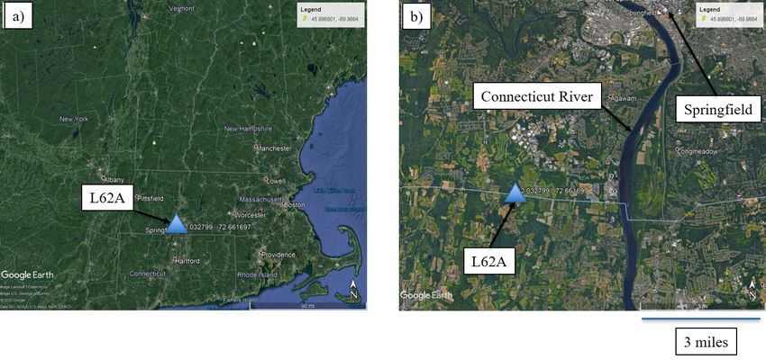
at frequencies
                                                            βi
                                                    fn =                                                   (2)
                                                            4di
where
 ui is the displacement of layer i
 uj is the displacement of layer j
 ρi is the density of layer i
 ρj is the density of layer j
 βi is the density of layer i
 βj is the density of layer j
 di is the thickness of layer i
 fn is the fundamental frequency
    From equation 1, which is referred to as the “impedance contrast” of the boundary between two layers,
lower density and velocity soil overlying higher density and velocity basement rock will amplify the sur-
face displacement relative to the basement displacement. Additionally, from equation 2, the fundamental
resonance of shaking will decrease with an increase in depth or a decrease in overburden S-wave velocity.
    The NEHRP site classification system is split up into 6 site classes, A-F each defined by a range of V s30
values (table 1). V s30 is defined as the average shear wave velocity of the top 30 meters of the soil profile
and is computed using the equation:
                                                       Pn
                                                             di
                                              V s30 = Pni=1 di                                             (3)
                                                            i=1 V si

where n is the number of layers, d is the depth of layer i and V s is the S-wave velocity of layer i. This
computation is performed for only the top 30 meters of the soil profile to compute V s30 but can be used
to compute the average S-wave velocity over any soil profile if the profile is not limited to only the top 30
meters.

                       Site Class    VS30 (m/s)               General Description
                           A           > 1500                     Hard rock
                           B          760-1500        Rock with moderate weathering
                           C          360-760           Very dense soil and soft rock
                           D          180-360                      Stiff soil
                           E           < 180                     Soft clay soil
                           F            N.A        Soils requiring site specific evaluations

                                    Table 1: NEHRP site classification system.

   The NEHRP site classification system provides a good first approximation for site effects. It does not,
however, capture some key information, specifically 1) depth to the significant impedance contrast and 2)
S-wave velocity information below 30 meters. Consider the following two shear wave velocity profiles: profile
1 and profile 2 (figure 1).

                                                        2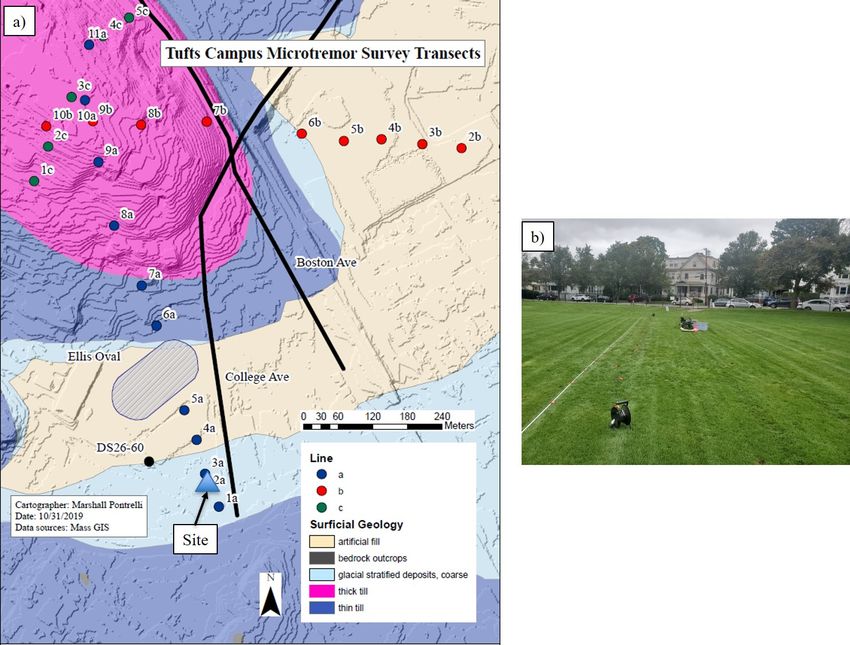
Figure 1: S-wave velocities for profiles 1 and 2. Shown are each profile’s depth to the impedance contrast,
impedance value (equation 1), V s30 (equation 3), fn (equation 2) and site class (table 1).

    Each has a single layer of 100 m/s S-wave velocity overlying a basement layer of 1000 m/s. Profile
1, however, is much shallower at a depth of 15 m whereas profile 2 is deeper at a depth of 100 meters.
Because the basement velocity is incorporated into the V s30 computation for profile 1, the V s30 is greater
than that of profile 2 and consequently, the site class is different: site class D instead of site class E. But is
profile 1 less susceptible to site effects than profile 2 as its site classification would indicate? In fact, their
impedances are the same and thus the maximum amplification of the site transfer function is the same, this
maximum amplification simply occurs at a different frequency (figure 2, note the profile used to generate this
figure includes soil damping of ζ = 2.5% which lowers the impedance. With no soil damping, the transfer
function amplification equals 15.9, the impedance in figure 1 computed from eq 1). Thus, the maximum
amplification of each of these profiles will affect buildings of different heights, but in similar amounts of
energy amplification. Using the back of the hand calculation of 0.1 s period per story to calculate building
fundamental resonance, a 6-story building at profile 1 and a 40-story building at profile 2 will be most
susceptible to amplification at its respective site. In each case, however, the amount of amplification at this
frequency is the same and thus, I argue, the two profiles should have the same site classification.

                                                        3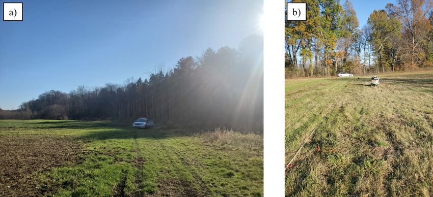
Figure 2: Theoretical transfer functions for profiles 1 and 2. The overburden and basement layer of each
profile has a density of 1.7 and 2.7 g/cm3 respectively. The overburden damping value for each profile is
ζ = 2.5%

2.0 Methods
In this study, I use two data collection and processing techniques, MASW and HVSR, and two forward
models both based of Thompson Haskell Propagator matrices (Thompson 1050, Haskell 1953, Haskell 1960,
Shearer 2017) to develop dispersion curves and SH1D theoretical transfer functions.

2.1 HVSR
2.1.1 Theory
The horizontal to vertical spectral ratio (HVSR) is an indirect way of approximating the surface-to-borehole
empirical transfer function (ETF) from a single surface recording by canceling out the Rayleigh wave and P-
wave influences on the surface record in order to enhance the image of the shear wave resonance (Nakamura,
1989). The surface ground motion is contaminated by surface waves, particularly Rayleigh waves, so the
magnitude response at a site is not a clear representation of shear wave content in the record. The HVSR
minimizes the effect of the Rayleigh wave on the surface recording to isolate the shear wave resonance,

                                                     4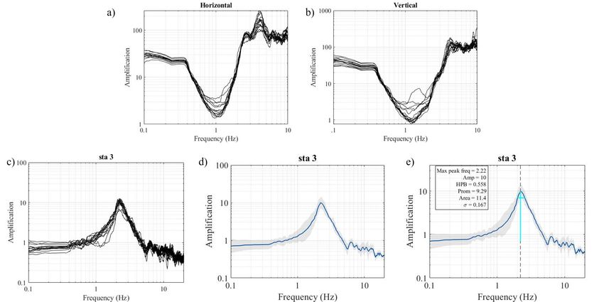
thus approximating both the fundamental frequency and amplification of multiple reflecting SH waves. The
amplification of vertically propagating shear waves is
                                                           Ha
                                                 a(f ) =                                                   (4)
                                                           Hb
where Ha is the horizontal magnitude response at a site on the ground surface, and Hb is the horizontal
magnitude response at a location at depth. This ratio is analogous to the surface-borehole transfer function.
The surface site, Ha , is influenced by Rayleigh waves, the amount of which relative to the bedrock site is
                                                                     Va
                                     Inf luenceof Rayleighwave =                                           (5)
                                                                     Vb
where Va is the vertical magnitude response at the surface site, and Vb is the vertical magnitude response at
the soil-bedrock interface site. This assumes that the Rayleigh wave particle ellipse dimensions are uniform
and scaled throughout the material (Fig. 3, maroon lines). Dividing the shear wave amplification by the
influence of the Rayleigh wave, therefore, removes the influence of the Rayleigh wave.
                                                                     Ha Vb
                                a(f )/Inf luenceof Rayleighwave =      ∗                                   (6)
                                                                     Hb Va
There is little amplification of multiple reflecting P-waves propagating from location the base to the surface
at the shear wave resonant frequency (fn ) because the P-wave has a higher velocity than the S-wave, thus
the P-wave fn will be higher than the S-wave fn . Similarly, Rayleigh waves influence the record at higher
frequencies than the S-wave fn . The ratio of the vertical motions at the S-wave fn is therefore approximately
1, while at higher frequencies, the correction normalizes out the Rayleigh wave and P-wave influences. The
Rayleigh and P-wave resonance peaks beyond the S-wave fn are therefore diminished without significantly
affecting the amplitude or shape of the fundamental peak. The S-wave fn and amplification at the surface
can therefore be approximated by the HVSR at the fundamental frequency (f0 ) as
                                                                Ha
                                             HV SR(f0 ) =                                                  (7)
                                                                Va
because Vb /Hb = 1. Equation 10 defines the horizontal to vertical spectral ratio.

                                                      5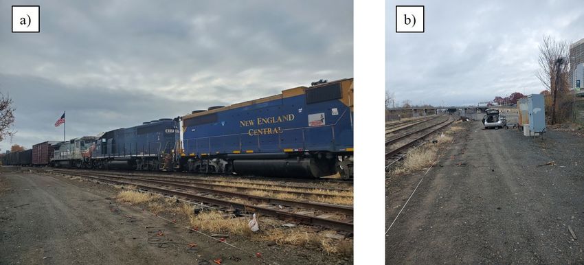
Figure 3: Retrograde Rayleigh waves traveling left to right across the page. The circles represent particles
and the arrows represent their motion. The ellipses show the continuous particle motion. The squares
represent locations a at the surface and b at depth. The maroon lines show the length of the long axis of
the Rayleigh wave ellipse at location a and at location b. The Rayleigh wave cartoon is based on Fig. 2.15
in Sheriff and Geldart 1995, second edition.

2.1.2 Data Processing
I collect 30 minutes of data in the field and filter the raw record using a fourth-order bandpass Butterworth
filter (Butterworth 1930) with a low corner of 0.1 Hz and a high corner of 49 Hz (figure 4). I then window the
data into 120 second windows, 1 second apart and compute the Fourier amplitude spectra of each component
of each window. I then combine the horizontal components using their geometric mean (SESAME 2004a)
and smooth the resulting horizontal and magnitude response vertical magnitude response using a 0.5 Hz
width smoothing filter (figure 5a and b). I then dive the components to get an HVSR of each window (figure
5c) and stack the 14 HVSRs and average them together using the log-normal maximum likelihood estimator
(figure 5d): (Thompson et al. 2009, Thompson et al. 2012, Steidl et al. 1996).
                                                          n
                                                     1X
                                   HV SRavg   = exp(       ln[HV SRi (f )])                                (8)
                                                     n i=1

where HV SRi (f ) is the HVSR(f) for i = 1, ..., n windows. I plot HV SRavg with a large sample 100(1 − α)
confidence interval:

                                  exp(ln[HV SRavg (f )] ± z1−α/2 ∗ σln (f ))                               (9)
with standard deviation:
                                       v
                                       u n
                                       u1 X
                            σln (f ) = t       (ln[HV SRi (f )] − ln[HV SR(f )])2                        (10)
                                         n i=1

                                                      6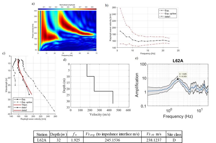
Finally, I measure different shapes in the HVSR fundamental peak (figure 5e).

                            Figure 4: Microtremor time series after processing.

Figure 5: Entire process of developing an HVSR. a and b) computing horizontal and vertical Fourier am-
plitude spectra of each window. c) computing the HVSR at each window. d) averaging the HVSR and
computing its confidence intervals using eqs 8-10. e) computing statistics describing the shape of the peak.

                                                     7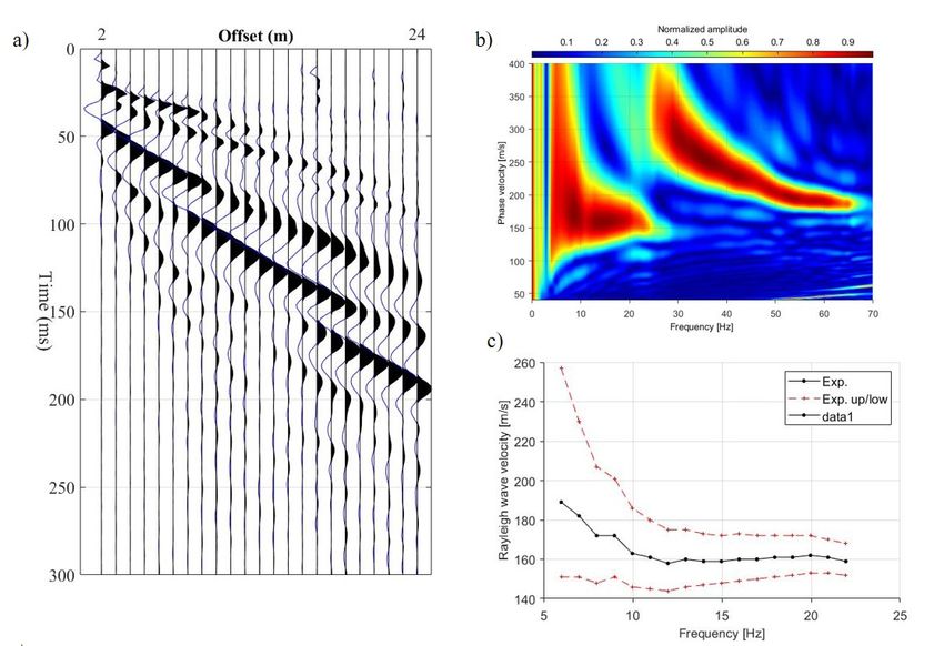
2.2 MASW
2.2.1 Theory
MASW, or multichannel analysis of surface waves, is a processing technique to pull wave dispersion infor-
mation out of a geophone line. The theory is laid out in Park et al. 1998b and begins in the (x-t) domain
with a geophone line shot gather. Each channel is transformed into the frequency domain using the Fourier
transform:
                                                   Z
                                        U (x, w) = u(x, t)eiwt dt                                    (11)

   It is then split into the phase and magnitude response:

                                         U (x, w) = P (x, w)A(x, w)                                      (12)
where P (x, w) is the phase and A(x, w) is the amplitude spectrum. P (x, w) contains all the phase information
so we break down eq. 11 further into:

                                          U (x, w) = e−iφx A(x, w)                                       (13)

   where Φ = w/cw , w = circular frequency in radians and cw = phase velocity at frequency w. We then
apply the transform:                   Z
                            V (w, φ) = e−i(Φ−φ)x [A(x, w)/|A(x, w)|]dx                           (14)

   Thus, by looping over values of φ at each frequency, the maximum value of V (w, φ) will be w/cw from
which we can solve for the phase velocity cw at the correct frequency (these equations are provided in more
detail in Park 1998b).

2.2.2 Data Processing
To compute dispersion curves practically in the field, I collect a shot gather with 2 meter offset and 1 meter
spacing using a geophone line of 24 4.5 Hz geophones collected using a Seistronix data acquisition unit and
a sledgehammer trigger. I then process the data using eqs. 11-14. A time domain plot of a gather is shown
in figure 6a below and the corresponding dispersion curve is figure 6b. I then select the maximum value of
the fundamental mode in the dispersion curve to develop my final dispersion curve (figure 6c).

                                                      8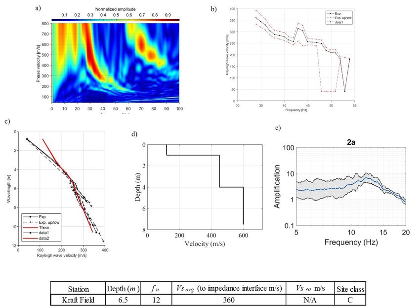
Figure 6: a) Shot gather for MASW processing. b) dispersion curve from shot gather in a. c) dispersion
curve picks from b.

2.3 SH1D TTF using Boore (2005) software
2.3.1 Theory
In site response studies, we often model the theoretical transfer function, hereafter TTF, with 1) vertically
propagating shear waves through 2) laterally homogenous soil layers that have 3) frequency independent
damping and 4) strain independent shear modulus, assumptions collectively referred to as “SH1D”. The
source input i(t), earth’s crust he (t), site geology hg (t), and instrument response hr (t) are linear time
invariant systems, and the recorded ground motion s(t) is a linear combination of these systems (figure 7):

                                      s(t) = i(t) ∗ he (t) ∗ hg (t) ∗ hr (t)                             (15)

where ∗ is the convolution operator (Borchert, 1970; Sheriff and Geldart, 1995). The Fourier response spectra
of the ground motion is equal to the product of the Fourier transform of each of the respective systems:

                                       S(f ) = I(f )He (f )Hg (f )Hr (f )                                (16)

An earthquake at a large hypocentral distance from the location of interest has vertically incident incoming
waves due to Snell’s law and the tendency of density to increase with depth in the Earth (Sheriff and Geldart,
1995). Two records in the basin, a on soil and b, on rock have equal source, path and instrument response,
thus the shear wave transfer function, a(f ), from location b to location a is the ratio of the magnitude
response spectra of the horizontal component of a and b.

                                                        9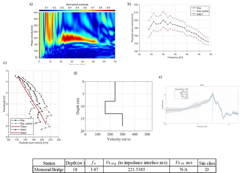
Sha (f )
                                               a(f ) =                                                    (17)
                                                         Shb (f )
where Sha (f ) is the horizontal component of the record at location a and Shb (f ) is the horizontal component
of the record at location b. This ratio is the site SH1D transfer function and we can model it using a forward
model or approximate it using data.

Figure 7: a) Site response model from a global seismological perspective with earthquake hypocenter, i(t),
represented by a red x, earth’s crust, he (t), represented by horizontal layers of varying color, site geology,
hg (t), represented by a brown basin, and instrument response, hr (t), represented by a black square. b) The
site geology, hg (t). c) The variables with which we model the site geology.

   The SH1D TTF is a function of the vibrational properties of the media through which the waves propa-
gate: the depth d,the shear wave velocity β, the density ρ and the attenenuation Q of the overburden, and
the velocity and density of the basement. For a more in depth discussion of Q see Shearer 2019.

                                                      10
2.3.2 Computation
To compute the theoretical transfer function, I use the Nrattle Fortran routine, which calculates the Thomson-
Haskell plane SH-wave transfer function (Thomson, 1950; Haskell, 1953) for horizontally stratified, laterally
homogenous layers with vertically propagating shear waves (written by C. Mueller with modification by
R. Herrmann and distributed in the Boore (2005) SMSIM ground motion simulation program). The input
parameters for Nrattle are a shear wave velocity profile (β), and corresponding depths (d), densities (ρ) and
attenuations (i Qs ) of the overburden; and the density and shear wave velocity of the basement. The outputs
of Nrattle are the TTF amplification as a function of frequency in Hz and is used to compute the curves in
figure 2.
3.0 Data
In this project, I use data from three sites, two in the Connecticut River Valley and one on the Tufts campus.
At each of these sites, I collected and processed microtremor data for the HVSR and geophone traces to
compute dispersion curves.
3.1 L62A
L62A was a transportable array station installed as part of the Earthscope project from 2013-2015. It is
located on Connecticut river flood plain sediments about 10 km south of Springfield. I found the local site
conditions to be swampy and the property it is on is farmland. A former undergraduate student at Tufts,
Justin Reyes, originally identified the site as exhibiting site amplification during a search for resonant New
England seismological stations he performed in 2019. This site is the only site of the three where instead of
collecting microtremor data, I used the data from the TA station.
Figure 8: a) Location of L62A within the Connecticut River Valley b) Higher resolution image showing
surrounding farmland on Connecticut River flood plain
11Figure 9: a) The field where L62A is, to the right and running behind the car is swampy, wet lowland. a)
L62A site.
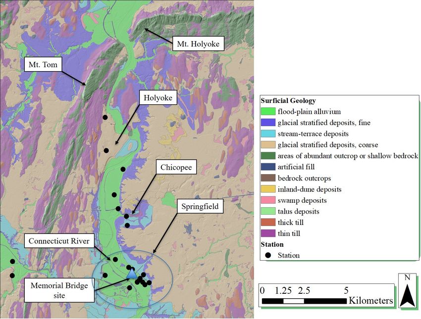
123.2 Memorial Bridge
The Memorial Bridge site is located just south of Memorial Bridge in Springfield on the East side of the
Connecticut River between the River and Route 91. Like L62A, it sits on the Connecticut River flood plain
sediments. It is adjacent to a train line and surrounded by various types of infrastructure: highway, bridge,
parking lot and others.
Figure 10: Memorial Bridge location within the greater area surficial geology
13Figure 11: a) Memorial bridge site adjacent train line b) Site with Memorial Bridge in the distance and
downtown Springfield to the right
143.3 Kraft Field
The Kraft field site is on the Tufts Medford-Somerville campus. The main portion of the campus (thick
till in figure) is a drumlin and the surrounding lower regions are a combination on artificial fill and glacial
outwash deposits. This site is located is located on about 6 meters of outwash deposits (figure 13) known
from drilling studies in Grant Garven’s hydrogeology class.
Figure 12: a) Kraft field site within local surficial geology b) Site
15Figure 13: Kraft Field well log from nearby site DS26-60 (figure ) drawn by Grant Garven and reinterpreted
by me.
4.0 Results
For each of the three sites, I developed an HVSR and a dispersion curve and inverted for the shear wave
velocity profile that fits the relationship in equation 2. This yields a 1) a depth to the impedance contrast, 2)
a fundamental frequency (computed from the data) and 3) and average velocity to the impedance contrast.
I also present the V s30 when the depth is greater the 30 meters (which is only at one site).
4.1 L62A
The dispersion curve for station L62A is clean with a clear fundamental and first mode. The higher modes
were clear too but are not shown in the figure. The fundamental phase velocities are just below 200 m/s.
The model I got that best fit this dispersion curve while conforming to the site fundamental resonance is a
roughly linearly increase shear wave velocity profile of 32 meters depth with an average velocity of 245.15
m/s. This has a V s30 of 238.12 m/s and is, by the traditional classification scheme, a site class D.
16Figure 14: a) Dispersion curve b) dispersion curve picks c) model fit d) shear wave velocity profile from the
model e) HVSR curve. Table) Results from analysis
4.2 Memorial Bridge
The Memorial bridge dispersion curve is significantly less clean than the L62A dispersion curve. There is
no clear evidence of higher modes and at frequencies below 20 Hz, the signal becomes incoherent. There is,
however, a clear fundamental mode at around 200 m/s. This mode, however, is concave down, indicating a
potential low velocity zone. Consequently, the model fit for this profile is not as good as the model fit for
L62A as I was unable to map the low velocity zone cleanly onto the dispersion curve. Despite the inability to
get a tight fit, however, we still get a good picture of the average shear wave velocity of the site of 221 m/s,
like that obtained at L62A. These sites are located in the same soil unit and thus it makes sense that their
average velocities are similar even though the Memorial bridge site is messier. My guess is that the mess at
Memorial Bridge is from the many infrastructural projects that have shaped and reshaped the subsurface.
17Figure 15: a) Dispersion curve b) dispersion curve picks c) model fit d) shear wave velocity profile from the
model e) HVSR curve. Table) Results from analysis
4.3 Kraft Field
The Kraft Field site is in a different geologic unit than L62A and Memorial bridge, glacial outwash instead of
river flood plain. There is evidence of the first mode in the dispersion curve, though is less clean than the first
mode in the L62A dispersion curve. Additionally, the phase velocities are significantly higher, between 300
and 800 m/s than the phase velocities in the other two sites with more steeply increasing phase velocities
towards lower frequencies. This, combined with a much higher fundamental frequency of 12 Hz yields a
shallower, higher shear wave velocity profile than the other two sites. The 6.5 meters I calculated for the
depth from the dispersion curve inversion is close to the 6 meters at the DS26-60 site that was found from
drilling a borehole, a good indicator that the inversion is pretty close to the actual profile.
18Figure 16: a) Dispersion curve b) dispersion curve picks c) model fit d) shear wave velocity profile from the
model e) HVSR curve. Table) Results from analysis
5.0 Discussion and conclusion
Using this combination of MASW dispersion inversion and HVSR fundamental frequency, I can compute
easily the depth and average shear wave velocity of a site, giving a better picture of the subsurface than V s30
in isolation. At the 3 sites studied in this project, the technique showed that at sites L62A and Memorial
Bridge, both within the Connecticut River flood plain sediments, the shear wave velocity profiles and depths
are similar, though the finer details of each site’s profile can be more complex. The inversion scheme works
for the Kraft field as well, obtaining higher velocities in the profile while predicting a depth close to a known
depth nearby. At each of the sites, I measured the fundamental site resonance using the HVSR and inverted
for the site shear wave velocity ensuring the relationship in eq. 2 was maintained. This yields, in addition
to fundamental resonance, average shear wave velocity and depth to the impedance contrast. These three
parameters, I think, better describe a site than V s30 in isolation because they account for frequency of
shaking and depths greater than 30 meters in a profile, providing engineers with a more complete picture
of the profile. Additionally, this technique only requires slightly more time, effort and equipment than a
V s30 measurement alone with the addition of 30 minutes of microtremor collection and HVSR processing,
a well-studied and easy process. The additional information this classification system provides allows for
better understanding of site resonance at a minimal extra cost than V s30 in isolation.
19References
Boore, D. M. (2005). SMSIM-Fortran Programs for Simulating Ground Motion from Earthquakes: Version
2.3-A of OFR 96-80-A. United States Department of the Interior. U. S Geological Survey.
Borcherdt, R.D., (1970). Effects of Local Geology on Ground Motion Near San Francisco Bay. Bulletin of
the Seismological Society of America. Vol. 60, No. 1, pp. 29-61.
Butterworth, S., (1930). On the theory of filter amplifiers. Exp. Wirel. Wirel. Eng. 7, 536–541.
Haskell N. A. (1953) The dispersion of surface waves on multilayered media. Bulletin of the Seismological
Society of America; 72:17–34.
Haskell, N. A. (1960). Crustal Reflection of Plane SH Waves. Geophysical Research 65(12): 4147-4150.
Kramer, S.L. (1996). Geotechnical Earthquake Engineering, Prentice Hall, Upper Saddle River, N.J.
Nakamura, Y. (1989) A Method for Dynamic Characteristics Estimation of Subsurface using Microtremor
on the Ground Surface. Railway Technical Research Institute 30(1): 25-33.
Olafsdottir, E.A., Erlingsson, S., Bessason, B. (2017). Tool for analysis of multichannel analysis of surface
waves (MASW) field data and evaluation of shear wave velocity profiles of soils. Can. Geotech J. 55: 217-233
(2018).
Park, C.B., Miller, R.D., Xia, J. (1998b). Imaging dispersion curves of surface waves on multi-channel record.
Kansas Geological Survey.
Park, C.B., Miller, R.D., Xia, J. (1999). Multichannel analysis of surface waves. Geophysics Vol 64, No.3,
p. 800-808.
SESAME (2004a). Guidelines for the implementation of the H/V spectral ratio technique on ambient
vibrations. European Commission - Research General Directorate.
SESAME (2004b). Site Effects Assessment Using Ambient Excitations. European Commission - Research
General Directorate. Project No. EVG1-CT-2000-00026 SESAME.
Shearer, P.M. (2019) Introduction to Seismology, 3rd edition. Cambridge University Press.
Sheriff, R.E., Geldart, L.P. (1995). Exploration Seismology, Second Edition. Cambridge University Press.
Steidl JH, Tumarkin AG, Archuleta RJ. (1996) What is a reference site? Bulletin of the Seismological Society
of America 1996;86(6):1733–48.
Thomson WT. (1950). Transmission of elastic waves through a stratified solid. Journal of Applied Physics:
21:89–93.
20You can also read