Nonlocal Image and Movie Denoising - Antoni Buades Bartomeu Coll Jean-Michel Morel
←
→
Page content transcription
If your browser does not render page correctly, please read the page content below
Int J Comput Vis (2008) 76: 123–139
DOI 10.1007/s11263-007-0052-1

Nonlocal Image and Movie Denoising
Antoni Buades · Bartomeu Coll · Jean-Michel Morel

Received: 11 April 2006 / Accepted: 7 March 2007 / Published online: 4 July 2007
© Springer Science+Business Media, LLC 2007

Abstract Neighborhood filters are nonlocal image and                    paid to the application of the statistical optimality crite-
movie filters which reduce the noise by averaging similar               rion for movie denoising methods. It will be pointed out
pixels. The first object of the paper is to present a uni-              that current movie denoising methods are motion compen-
fied theory of these filters and reliable criteria to compare           sated neighborhood filters. This amounts to say that they
them to other filter classes. A CCD noise model will be                 are neighborhood filters and that the ideal neighborhood of
presented justifying the involvement of neighborhood fil-               a pixel is its trajectory. Unfortunately the aperture prob-
ters. A classification of neighborhood filters will be pro-             lem makes it impossible to estimate ground true trajecto-
posed, including classical image and movie denoising meth-              ries. It will be demonstrated that computing trajectories and
ods and discussing further a recently introduced neighbor-              restricting the neighborhood to them is harmful for denois-
hood filter, NL-means. In order to compare denoising meth-              ing purposes and that space-time NL-means preserves more
ods three principles will be discussed. The first principle,            movie details.
“method noise”, specifies that only noise must be removed
from an image. A second principle will be introduced,                   Keywords Image denoising · Movie denoising · Motion
“noise to noise”, according to which a denoising method                 estimation
must transform a white noise into a white noise. Contrar-
ily to “method noise”, this principle, which characterizes
artifact-free methods, eliminates any subjectivity and can be
                                                                        1 Introduction
checked by mathematical arguments and Fourier analysis.
“Noise to noise” will be proven to rule out most denoising
methods, with the exception of neighborhood filters. This               1.1 Neighborhood Filters
is why a third and new comparison principle, the “statistical
optimality”, is needed and will be introduced to compare the            The main objective of this paper is to set under a common
performance of all neighborhood filters.                                framework and give comparison principles to all neighbor-
    The three principles will be applied to compare ten dif-            hood filters, including movie filters which are usually treated
ferent image and movie denoising methods. It will be first              as a different class. We shall call neighborhood filters all im-
shown that only wavelet thresholding methods and NL-                    age and movie filters which reduce the noise by averaging
means give an acceptable method noise. Second, that neigh-              similar pixels. General CCD noise models (briefly presented
borhood filters are the only ones to satisfy the “noise to              in Sect. 2) imply that noise in digital images and movies is
noise” principle. Third, that among them NL-means is clos-              signal dependent. Fortunately two pixels which received the
est to statistical optimality. A particular attention will be           same energy from the outdoor scene undergo the same kind
                                                                        of perturbations and therefore have the same noise model.
                                                                        Under the fairly general assumption that at each energy level
A. Buades · B. Coll · J.-M. Morel ()                                   the noise model is additive and white, denoising can be
CMLA (Mathematics), Ecole Normale Supérieure, de Cachan,
61 av. President Wilson, Cachan 94235, France
                                                                        achieved by first finding out the pixels which received the
e-mail: morel@cmla.ens-cachan.fr                                        same original energy and then averaging their observed grey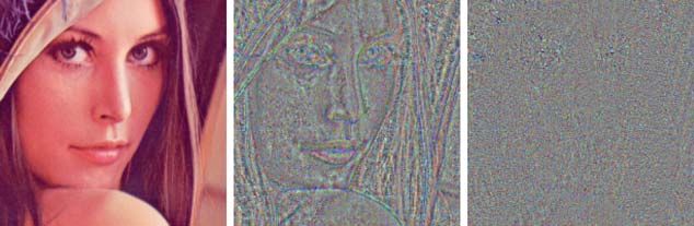
124                                                                                               Int J Comput Vis (2008) 76: 123–139

levels. This observation has led to the wide class of neigh-        improves significantly by forgetting about trajectories and
borhood filters classified in (Yaroslavsky 1985). Since the         using all similar pixels in space-time, no matter how many
original image value is lost these filters proceed by picking       are picked per frame. For this reason the NL-means filter
for each pixel i the set of pixels J (i) spatially close to i and   treats movies as a union of images, rather than an image se-
with a similar grey level value.                                    quence. The time ordering of this union is irrelevant. The
    Neighborhood filters proceed by replacing the grey              aperture problem results in the existence of more samples
 value of i, u(i), by the average N F u(i) = |J (i)| ×
                                                           1
level                                                               for each pixel and therefore increases the denoising perfor-
   j ∈J (i) u(j ). (Depending on the noise model other statis-      mance by nonlocal means.
tical estimates are of course possible like the median, etc.)
Under the assumption that pixels j ∈ J (i) indeed received
the same original energy as i, N F u(i) is a denoised version       1.4 Three Comparison Principles
of u(i). The more famous neighborhood filters are Lee’s
σ -filter (Lee 1983), SUSAN (Smith and Brady 1997) and              A systematic comparison of the huge variety of denoising
the bilateral filter (Tomasi and Manduchi 1998) where the           methods is requested. On the other hand a comparison be-
neighborhoods are Gaussian in space and grey level.                 tween methods which are based on very different principles
                                                                    cannot be performed without formal comparison criteria. Vi-
1.2 Non Local Means
                                                                    sual comparison of artificially noisy images with their de-
In a recent communication (Buades et al. 2005b) (see also           noised version is subjective. Tables comparing distances of
Buades et al. 2005a for a mathematical analysis) the authors        the denoised image to the original are useful. They have two
of the present paper extended the above mentioned neigh-            drawbacks, though. The added noise is usually not realis-
borhood filters to a wide class which they called non-local         tic, generally a white uniform noise with too large variance.
means (NL-means). This algorithm class defines the neigh-           Such comparison methods depend strongly on the choice of
borhood J (i) of i by the condition: j ∈ J (i) if the grey level    the image and do not permit to address the main issues: the
of a whole window around j is close to the grey level of the        loss of image structure in noise and the creation of artifacts.
window around i. The spatial constraint is instead relaxed.             Thus we shall apply three principles aiming at more ob-
   NL-means filters can be given two origins beyond classi-         jective benchmarks. The first principle (already presented in
cal neighborhood filters. The same Markovian pixel similar-         Buades et al. 2005b) asks that noise and only noise be re-
ity model was used in the seminal paper (Efros and Leung            moved from an image. It has to be perceptually tested di-
1999) for texture synthesis from a texture sample. In that          rectly on an image with no artificial noise added. The com-
case the neighborhood J (i) is not used for denoising. The
                                                                    parison of methods is performed on the difference between
aim was to estimate from the texture sample the law of i
                                                                    the image and its denoised version. We called this differ-
knowing its neighborhood. This law is used to synthesize
                                                                    ence method noise. It is much easier to evaluate whether a
similar texture images by an iterative algorithm.
                                                                    method noise contains some structure removed from the im-
1.3 Movie Denoising                                                 age or not. The outcome of such experiments is clear cut on
                                                                    a wide class of denoising filters of all origins including all
Last but not least, most state of the art movie denois-             mentioned neighborhood filters.
ing methods are neighborhood filters and some of them,                  We shall introduce here a second principle, noise to
in some sense, NL-means filters. Indeed, motion compen-             noise, which requires that a denoising algorithm transforms
sated denoising methods start with the search for a temporal        a white noise into a white noise. This paradoxical require-
neighborhood J (i), the trajectory, followed by an averaging        ment seems to be the best way to characterize artifact-free
process. By the Lambertian assumption a pixel belonging
                                                                    algorithms. It is affordable to mathematical analysis and to
to a certain object conserves the same grey level value dur-
                                                                    Fourier spectrum testing. Mathematical and experimental ar-
ing its trajectory. Therefore this is computed as a grey level
                                                                    guments will show that bilateral filters and NL-means are
neighborhood of i in the sense of neighborhood filters. The
                                                                    the only ones satisfying the noise to noise principle.
comparison of grey levels is not a sufficient criterion, a diffi-
culty usually called the aperture problem. Thus several mo-             The third principle, the statistical optimality is restricted
tion compensated filters involve block matching. They con-          to neighborhood filters. It questions whether a given neigh-
struct J (i) by comparing a whole block around j to a whole         borhood filter is able or not to retrieve faithfully the neigh-
block around i.                                                     borhood J (i) of any pixel i. NL-means will be shown to
   In all of these movie denoising algorithms the neighbor-         best match this requirement. We shall apply this principle to
hood J (i) picks a single pixel per frame. One of our objec-        demonstrate that, contrarily to the current dominant technol-
tives is to prove that this restriction is actually counterpro-     ogy, motion estimation or compensation is not needed, and
ductive. In fact the performance of movie denoising filters         even harmful, to perform movie denoising.
Int J Comput Vis (2008) 76: 123–139                                                                                         125

1.5 The Extension of Patch-based Denoising Methods                all similar blocks are put into a single 3D volume, where
                                                                  time is replaced by a similarity order. We may anticipate that
Since a first version (Buades et al. 2005c) of the present pa-    our conclusions are similar to the conclusions of (Dabov et
per was disclosed in May 2005, several variants of nonlocal,      al. 2006). Applied to a movie, their algorithm will lead to
or “patch-based” methods and very careful denoising bench-        substitute to the movie time a “similarity time”, where all
marks have been published by several authors. Mahmoudi            blocks are put after each other based on their similarity and
and Sapiro (2005) reported excellent denoising results and        not on their time order. This yields much more redundancy,
acceleration methods for the non local means algorithms           and therefore to a better denoising.
applied to images and movies. Kervrann and Boulanger
(2006), Boulanger et al. (2006) proposed an adaptive exten-       1.6 Plan
sion of NL-means with variable window size depending on
statistical estimates, and performed an impressive compar-        We shall proceed as follows. Section 2 presents a realistic
ison benchmark. Awate and Whitaker (2005) have simulta-           CCD noise model which leads to the basic hypothesis jus-
neously proposed a method whose principles stand close to         tifying neighborhood filters. Neighborhood filters including
the NL-means algorithm, since the method involves com-            NL-means and motion compensated movie denoising filters
parison between subwindows to estimate a restored value.          are defined in Sect. 3. This section describes and discusses
The objective of the algorithm “UINTA, for unsupervised           some main movie filters. Section 4 proposes the three prin-
information theoretic adaptive filter”, is to denoise the im-     ciples to evaluate the performance of any denoising method.
age by decreasing the randomness of the image. Azzabou et         All three principles are designed to serve comparative exper-
al. (2006) have proposed an acceleration of NL-means by a         iments. Finally, the last section is devoted to a more mathe-
random walk exploration around each pixel and have again          matical comparison of classical neighborhood filters and the
reported impressive results for this accelerated NL-means.        NL-means.
Kindermann et al. (2005) and Gilboa et al. (2006) have given
a new, variational framework to non-local denoising leading
to iterated algorithms. They have also performed extensive        2 Noise Model
comparisons with total variation denoising.
    Probably the most impressive results for a block match-       Most digital images and movies are obtained by a CCD de-
ing based denoising have been just reported by Dabov et al.       vice. Following (Colleen Gino 2004; Howell 2000; Gonza-
(2006). Let us summarize their methods in their own terms:        lez and Woods 2002), CCD’s show three kinds of noise. The
(We start by) “grouping similar 2D image fragments (e.g.          first one is the shot noise proportional to the square root of
blocks) into 3D data arrays called “groups”. Collabora-           the number of incoming photons in the captors during the
                                                                  exposure time, namely
tive filtering is a special procedure developed to deal with
these 3D groups. We realize it using the three successive
                                                                           Φ
steps: 3D transformation of 3D group, shrinkage of trans-         n0 =        t · A · η,
                                                                           hν
form spectrum, and inverse 3D transformation. The result is
a 3D estimate that consists of the jointly filtered grouped im-   where Φ is the light power (W/m2 ), hν the photon energy
age blocks. By attenuating the noise, the collaborative filter-   (W s), t the exposure time in seconds (s), A the pixel area
ing reveals even the finest details shared by grouped blocks      (m2 ) and η the quantum efficiency. The√other constants be-
and at the same time it preserves the essential unique fea-       ing fixed we can simply retain n0 = c Φ where Φ is the
tures of each individual block. The filtered blocks are then      “true image” and C a constant (see Fig. 1).
returned to their original positions. Because these blocks           Second, a dark or obscurity noise n1 is due to spurious
are overlapping, for each pixel we obtain many different          photons produced by the captor itself. We can assume the
estimates which need to be combined. Aggregation is a             dark noise to be white, additive and with zero mean. The
particular averaging procedure which is exploited to take         zero mean property is due to the substraction of a dark frame
advantage of this redundancy. (...) The experimental re-          from the raw image. The dark frame is obtained by averag-
sults presented here demonstrate that the developed meth-         ing the obscurity noise over a long period of time.
ods achieve state-of-the-art denoising performance in terms          Third, the read out noise n2 is another electronic additive
of both peak signal-to-noise ratio and subjective visual qual-    and signal independent noise. This noise can be assumed to
ity.”                                                             have zero mean by the substraction from the raw image of a
    The most striking point of this method is the fusion of       bias frame.
NL-means with a transform-domain shrinkage. The main                 Digital images eventually undergo a “gamma” correc-
step remains block matching, but then the process is anal-        tion, i.e. a nonlinear increasing contrast change g: “Gamma
ogous to a motion compensated movie denoising algorithm:          correction is the name of an internal adjustment made in the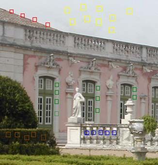
126                                                                                                  Int J Comput Vis (2008) 76: 123–139
Fig. 1 Simulated shot noise.
Left: original√image u. Right:
noise image un where n is the
realization of a zero mean white
noise with standard deviation
σ = 1. The noise in bright parts
is larger than in dark parts, an
effect which is corrected and
sometimes reversed by
gamma-correction

rendering of images through photography, television, and              Hypothesis 1 In a digital image, the noise model at each
computer imaging. The adjustment causes the spacing of                pixel i only depends on the original pixel value Φ(i) and is
steps of shade between the brightest and dimmest part of an           additive. Let J (i) be the set of pixels with the same original
image to appear “appropriate” (Gonzalez and Woods 2002).              value as i. Then n(j ), j ∈ J (i) are independent and identi-
Summarizing,                                                          cally distributed.

u(i) = g(Φ(i) + c Φ(i)n0 (i) + n1 (i) + n2 (i)),                          Hypothesis 1 cannot be used directly because Φ(i) is
                                                                      unknown. The challenge is to find out J (i) for every i.
where u(i) is the observed intensity at a pixel i, Φ(i) the           The simplest idea to do so is to assume that all pixels with
“true physical” light intensity average power sent by the             the same observed value u(i) have the same noise model.
scene to pixel i, c a constant, n0 (i), n1 (i) and n2 (i) three       A more sophisticated use of Hypothesis 1 is the follow-
independent and signal independent white noises. In prac-             ing: for a given pixel in an image, detect all pixels which
      √ = s with 0 < α < 1. When Φ(i) is large the shot
tice g(s)    α
                                                                      have the same underlying model. By Hypothesis 1 each j
noise Φ(i) dominates n1 and n2 and is dominated by the                in J (i) obeys a model u(j ) = v(i) + n(j ) where n(j ) are
signal Φ(i). Thus we can expand u(i) as                               i.i.d. It is then licit to perform
                                                                                                         a denoising of u(i) by re-
                                                                     placing it by N F u(i) =: |J 1(i)| j ∈J (i) u(j ). By the vari-
u(i)  g(Φ(i)) + g  (Φ(i))(c Φ(i)n0 (i) + n1 (i) + n2 (i))           ance formula for independent variables one then obtains
      =: g(Φ(i)) + n(i).                                        (1)   N F u(i) = v(i) + ñ(i) where
                                                                                        1
If instead Φ(i) is small with respect to n1 (i) + n2 (i),             Var(ñ(i)) =           Var(n(i)).                             (4)
                                                                                     |J (i)|
n(i)  u(i)  g(n1 (i) + n2 (i)).                               (2)   By (4) if nine pixels with the same color plus some uncorre-
                                                            1         lated noise are averaged the noise is divided by three. Algo-
Let us mention a case of particular interest. If g(s)  s , the
                                                            2
                                                                      rithms proceeding in this way will be called neighborhood
noise n(i) reads                                                      filters. We shall now examine several classical or new in-
                                                                     stances.
         n0 (i)             in the bright parts of the image,
n(i)  √
            n1 (i) + n2 (i) in the dark parts of the image.
                                                                (3)   3 General Neighborhood Filters

   In all cases the noise is signal dependent but independent         3.1 Local Neighborhood Filters
at different pixels. Figure 1 displays a simulated shot noise
associated to the Lena image. This noise is signal dependent          The more primitive neighborhood filters replace the color of
and much stronger in bright regions than in dark regions. In          a pixel with an average of the nearby pixels colors. Thus
order to apply many computer vision algorithms, the noise             J (i) is a spatial neighborhood. The filtered value can be
parameters must be first estimated. For the study of these            written as
parameters for the previous real CCD model we refer the                                              2
                                                                                    1         − |x−y|
reader to (Liu et al. 2006).                                          Mρ u(x) =             e     ρ 2 u(y)dy,
                                                                                   πρ 2 R2
   In the following we aim at recovering g(Φ(i)), namely
the true image up to the unknown gamma correction. Equa-              where the parameter ρ is roughly the size of the spatial
tions (1), (2) and the white noise and independence assump-           neighborhood involved in the filtering. Now, the closest pix-
tions on n0 , n1 and n2 legitimate the following hypothesis:          els to i have not necessarily the same color as i. For instance
Int J Comput Vis (2008) 76: 123–139 127
Fig. 2 The nine pixels in the
baboon image on the left have
been enlarged. They present a
high red-blue contrast. In the red
pixels, the first (red) component
is stronger. In the blue pixels,
the third component, blue,
dominates. Neighborhood filters
select pixels with the same color
for averaging. In this case the
neighborhood of the central
pixel should contain the six red
pixels or, still better, the pixels
of the central column
and Manduchi 1998) make this process more symmetric by
involving a “bilateral” Gaussian depending on both space
and grey level. This leads to
2
− |x−y|
2
1 − |u(y)−u(x)|
SNF h,ρ u(x) = e ρ2
e h2 u(y)dy.
C(x)
There is another way to avoid the blurring effect of the spa-
tial filtering Mρ by a statistical correction which we are go-
ing to use in the sequel. When the Gaussian mean is per-
formed on an edge, the variance of the performed mean can
become larger than the variance of the noise. This is a clue
that the average is not licit. A statistically optimal correction
was proposed by Lee again (Lee 1980),
Fig. 3 Most image details occur repeatedly. Each color indicates a
σx2
group of squares in the image which are almost indistinguishable. Im- LMρ u(x) = Mρ u(x) + (u(x) − Mρ u(x)),
age self-similarity can be used to eliminate noise. It suffices to average σx2 + σ 2
the squares which resemble each other
where
2
the red pixel placed in the middle of Fig. 2 has five red neigh- 1 − |x−y|
bors and three blue ones. If its color is replaced by the av- σx2 = max 0, 2 e ρ 2
(u(y) − Mρ u(x)) dy − σ
2 2
πρ R2
erage of the colors of its neighbors, it turns blue. The same
process would likewise redden the blue pixels of this figure. and σ is the noise standard deviation. The original noisy
Thus, the border between red and blue would be blurred. values are less altered when the variance of the performed
In order to denoise the central red pixel, it is better to mean dominates the variance of the noise. This happens near
average the color of this pixel with the nearby red pixels the edges or in textured regions. In consequence, the noise
and only them, excluding the blue ones. This is exactly the is mainly reduced in flat zones as displayed in Fig. 4.
technique of the sigma-filter. This famous algorithm is gen- The bilateral filters perform a better denoising than Lee’s
erally attributed to Lee (1983) but can be traced back to correction. They maintain sharp boundaries, since they av-
Yaroslavsky and the Soviet Union image processing school erage pixels belonging to the same region as the reference
(Yaroslavsky 1985). The idea is to average neighboring pix- pixel. Bilateral filters fail when the standard deviation of
els which also have a similar color value. The filtered value the noise exceeds the edge contrast. This fact is more ex-
by this strategy can be written tensively exposed in Sect. 5. In the following experiments
we do not distinguish between the classical neighborhood
2
1 − |u(y)−u(x)| filter and SUSAN or the bilateral filter. The following expe-
NF h,ρ u(x) = e h2 u(y)dy, (5) riments have been performed using a fixed spatial neighbor-
C(x) Bρ (x)
hood and a Gaussian weighted grey level difference.
where u(x) is the color at x and NF h,ρ u(x) its denoised ver- Let us finally mention that the mean operation can be re-
sion. Only pixels inside Bρ (x) are averaged, h controls the placed by nonlinear operator like the median filter. The me-
color similarity and C(x) is the normalization factor. SU- dian filter (Tukey 1977) chooses the median value, that is,
SAN (Smith and Brady 1997) and the bilateral filter (Tomasi the value which has exactly the same number of grey level128 Int J Comput Vis (2008) 76: 123–139
Fig. 4 Comparison of neighborhood filters. From top to bottom and left to right: noisy image (σ = 15), Gaussian filtering, anisotropic filtering,
Lee’s statistical filter, sigma or bilateral filter and the NL-means algorithm. All methods except the Gaussian filtering maintain sharp edges.
However, the anisotropic filtering removes small details and fine structures. These features are nearly untouched by Lee’s statistical filter and
therefore completely noisy. The comparison of noisy grey level values by the sigma or bilateral filter is not so robust and irregularities are created
on the edges. The NL-means better cleans the edges without losing too many fine structures and details
values above and below in a fixed neighborhood. The me- edges which appear in most images. In 1999 Efros and Le-
dian filter preserves the main boundaries, but it tends to re- ung (1999) used non local self-similarities as the ones illus-
move the details. This filter is optimal for the removal of trated in Fig. 3 to synthesize textures and to fill in holes in
impulse noise on images and doesn’t blur edges. It is equiv- images. Their algorithm scans a vast portion of the image in
alent to an average of the pixels in a direction orthogonal to search of all the pixels that resemble the pixel in restoration.
the gradient, that is to an anisotropic diffusion or mean cur- The resemblance is evaluated by comparing a whole win-
vature motion (Merriman et al. 1992). In the following, we dow around each pixel, not just the color of the pixel itself.
shall also show experiments based on the mean curvature Applying this idea to neighborhood filters leads to a gener-
motion implemented as originally proposed in (Alvarez et alized neighborhood filter which we called non-local means
al. 1993). For a more recent review of the subject see (Keel- (or NL-means) (Buades et al., Buades et al. 2005a, 2005b).
ing and Stollberger 2002). NL-means has a formula quite similar to the sigma-filter,
Figure 4 compares the performance of the various con- (Gρ ∗|u(x+.)−u(y+.)|2 )(0)
sidered local neighborhood filters on a noisy image. Even if 1 −
NLu(x) = e h2 u(y)dy, (6)
each method provides a reasonable solution (all except the C(x) Ω
Gaussian filtering maintain sharp edges), none of them is
where Gρ is the Gauss kernel with standard deviation ρ,
fully acceptable. The anisotropic filter removes small details
C(x) is the normalizing factor, h acts as a filtering parameter
and fine structures. These features are nearly untouched by
and
Lee’s statistical filter and therefore completely noisy. The
bilateral filters create irregularities on the edges and leave (Gρ ∗ |u(x + .) − u(y + .)|2 )(0)
some residual noise on flat zones.
= Gρ (t)|u(x + t) − u(y + t)|2 dt.
R2
3.2 Nonlocal Averaging
The formula (6) means that u(x) is replaced by a weighted
The most similar pixels to a given pixel have no reason to average of u(y). The weights are significant only if a
be close to it. Think of periodic patterns, or of the elongated Gaussian window around y looks like the correspondingInt J Comput Vis (2008) 76: 123–139 129
Fig. 5 Comparison of different
denoising methods on a text
image. Top: noisy image. Below
and from left to right: crop of
the noisy image, the total
variation minimization, the
stationary wavelet thresholding,
the neighborhood filter with
spatial neighborhood 11 × 11
and the NL-means with the
whole image as search window.
NL-means seems well adapted
to text denoising since
characters and combinations of
characters are easily repeated in
a text. Since we have used only
three paragraphs the result can
be substantially improved by
using a complete page or even
more pages. In that case the
problem would be the huge time
of computation
Gaussian window around x. Thus the non-local means al- by an Euclidean norm of their difference. Indeed, if the noise
gorithm uses image self-similarity to reduce the noise as samples are locally i.i.d. with zero mean and variance σ 2 ,
illustrated in Fig. 4. As Fig. 5 shows, the NL-means seems
to be well adapted to text denoising since characters and Eu(Ni ) − u(Nj )2 = u0 (Ni ) − u0 (Nj )2 + 2σ 2 ,
combinations of characters are easily repeated in a text. One
of the limitations of the NL-means algorithm is the removal where u0 denotes the original (unknown) image and u the
of highly structured noise as in jpeg compressed images (see
noisy one obtained by the addition of a white noise. Thus
Fig. 6). The NL-means is able to remove the block artifact
using a threshold function and setting this hard threshold to
due to compression but at the cost of removing some de-
2σ 2 leads to take an average of pixels which originally had
tails as the difference between the compressed and restored
an almost identical window around them.
images shows.
So the point is: why using a soft Gaussian threshold in-
3.3 NL-Means Implementation Details stead of a hard one? We may find pixels for which there is
no identical or nearly identical window in the image. In that
A NL-means simple version averages pixels which have a case, the threshold strategy should leave exactly the noise
grey level window around at a distance less or equal than a value at such points. The result would visually be identified
certain threshold. The comparison of both windows is made as an impulse noise and the noise to noise principle would130 Int J Comput Vis (2008) 76: 123–139
Fig. 6 Application of NL-means to restore a highly compressed image. Top: compressed and restored image by NL-means. Bottom: detail of
previous images and its difference. NL-means is able to remove block artifacts due to compression but at the cost of removing some details, as the
difference between the compressed and restored image shows
be violated. An exponential function is used instead of the 3.4 Movie Denoising
threshold and makes a more adaptive weighting distribution.
The Euclidean distance between two windows is also Nearly all state of the art movie filters are motion compen-
weighted by a Gaussian-like kernel decaying from the cen- sated. The underlying idea is the existence of a “ground
ter of the window to its boundary. Indeed in digital images, true” physical motion, which motion estimation algorithms
closer pixels are more dependent and therefore closer pix- should be able to estimate. Legitimate information should
els to the reference one should have more importance in the exist only along these physical trajectories. The motion com-
pensated filters estimate explicitly the motion of the se-
window comparison. In order to involve the current pixel in
quence by a motion estimation algorithm. The motion com-
its own average, the distance between the window centered
pensated movie yields a new stationary data on which a sta-
at the reference pixel and itself is set equal to the minimum tic filter can be applied.
of the other distances. Otherwise, the probability distribu- One of the major difficulties in motion estimation is
tion should be excessively large at the pixel itself. the ambiguity of trajectories, the so called aperture prob-
For computational purposes of the NL-means algorithm, lem. This problem is illustrated in Fig. 8. At most pixels,
we can restrict the search of similar windows in a larger there are several options for the displacement vector. All
“search window” of size S × S pixels. In all experiments of these options have a similar grey level value and a simi-
we have fixed a 21 × 21 pixels search window and a simi- lar block around them. Now, motion estimators have to se-
larity square neighborhood of 7 × 7 pixels (this can be re- lect one by some additional criterion. The most classical
duced for color images). If the image has a size N × N , approaches to motion estimation are the optical flow con-
then the final complexity of the algorithm is about 49 × straint (OFC) based methods and the block matching algo-
rithms. OFC methods assume that the grey level value of
441 × N 2 . The acceleration of the algorithm by multireso-
the objects during their trajectory is nearly constant (Lam-
lution strategies has been proposed in (Buades et al. 2005a;
bertian assumption). In order to obtain a unique flow they
Mahmoudi and Sapiro 2005).
impose the flow field to vary smoothly in space. There
The filtering parameter h has been fixed to k ∗ σ with k ∈ has been a constant progress in this estimation Horn and
[0.75, 1], when a noise of standard deviation σ is added. Due Schunck (1981), Nagel (1983), Weickert (1998), Weickert
to the fast decay of the exponential kernel, large Euclidean and Schnörr (2001). Other constraints enforcing the con-
distances lead to nearly zero weights acting as an automatic stancy of the gradient and the Laplacian can be added as
threshold (see Figs. 16 and 18). proposed in Papenberg et al. (2006).Int J Comput Vis (2008) 76: 123–139 131
Fig. 7 Three consecutive
frames of a degraded image
sequence. The sparse time
sampling in film sequences
makes restoration more difficult
than in 3D images
main problem, motion estimation, can be circumvented. In
denoising, the more samples we have the happier we are.
The aperture problem is just a name for the fact that there
are many blocks in the next frame similar to a given one
in the current frame. Thus, singling out one of them in the
next frame to perform the motion compensation is an unnec-
essary and probably harmful step. A much simpler strategy
which takes advantage of the aperture problem is to denoise
a movie pixel by involving indiscriminately spatial and tem-
Fig. 8 Aperture problem and the ambiguity of trajectories are the poral similarities: let the best win! In that way, we propose
most difficult problem in motion estimation: There can be many good
to apply the NL-means to a movie in the following way:
matches. The motion estimation algorithms must pick one
(G ∗|u(x+.,t)−u(y+.,s)|2 )(0)
1 − ρ
NLu(x, t) = e h2
The second class of motion estimation algorithms com- C(x, t) Ω R
putes the displacement at each pixel by comparing the grey × u(y, s)dyds. (7)
level values in a whole block around it. The similarity is
measured by a l 1 or a l 2 distance. As Fig. 8 shows, there can Notice that the Gauss kernel Gρ is 2D but the integral in-
be many blocks with similar configurations in the reference volves time and space. In practical terms NL-means takes
frame. a spatial block around pixel x in frame t and looks for all
Once the motion compensation has been performed one similar blocks in all frames including the current one. Then
can classify the movie denoising methods by the kind of 3D a weighted average of all the similar pixels (y, s) is per-
neighborhood filter they apply to the compensated movie. formed. Figure 9 compares NL-means with motion compen-
We refer to (Brailean et al. 1995) for a comprehensive re- sated neighborhood filters. The NL-means also reduces mo-
view. Samy (1985) and Sezan et al. (1991) proposed the tion blur since it is not affected by possible errors of motion
LMMSE filter which is a motion compensated Lee’s filter. estimation algorithms.
Ozkan et al. (1993) proposed the AWA filter, a motion com-
pensation of the neighborhood filters. Huang (1981) and
Martinez (1986) implemented motion compensated median 4 Three Principles for Denoising Algorithms
filters. Motion compensated Wiener filters were earlier pro- Evaluation
posed by Kokaram (1993).
In this section, we shall address the problem of comparing
Figure 9 illustrates the improvement of motion compen-
different denoising methods by proposing three formal com-
sated algorithms compared with their static version. The
parison criteria.
static filters are obtained by extending the 2D image filter
support to the 3D time-space support. We call them static 4.1 Method Noise
because they do not take into account the dynamic character
of image sequences. As this figure illustrates, the details are A difference between the original image and its filtered ver-
better preserved and the boundaries less blurred with mo- sion shows the “noise” removed by the algorithm. This pro-
tion compensation. This explains why most recent papers cedure has been introduced recently in Buades et al. (2005a)
propose motion compensated algorithms. and this difference or residue is called method noise. In
principle the method noise should look like a noise. Oth-
3.5 Nonlocal Means for Movies erwise, the method noise can be filtered again and its de-
terministic part turned back to the image. Recent denois-
The above description of movie denoising algorithms and ing methods adopted this recursive strategy to recover im-
its juxtaposition to the NL-means principle shows how the age information lost in method noise (Osher et al. 2005;132 Int J Comput Vis (2008) 76: 123–139
Fig. 9 Comparison of static filters, motion compensated filters and NL-means applied to the sequence of Fig. 7. Only a piece of the central
frame is displayed. From top to bottom and left to right: Lee’s correction, Lee’s correction with block matching (BM)-(LMMSE), sigma filter and
sigma filter with block-matching (AWA). Middle: the noise removed by each method (difference between the noisy and filtered frame). Motion
compensation improves the static algorithms by better preserving the details and creating less blur. The noise removed by LMMSE is nearly zero
on the strong boundaries. Thus, these boundaries are kept noisy. We can read the titles of the books in the noise removed by AWA. Therefore,
that much information has been removed from the original. Finally, the NL-means algorithm (bottom row) has almost no noticeable structure in its
removed noise. As a consequence, the filtered sequence has kept more details and is less blurred
Tadmor et al. 2004). When the standard deviation of the gorithms are applied to a slightly noisy version of the image
noise is higher than the feature contrast a visual exploration (σ = 2.5). Method parameters are fixed so that the method
of the method noise is not reliable. Image features can be noise has exactly σ 2 variance per pixel. The same parame-
masked in method noise. Thus the evaluation of a denoising ters have been used in the second experiment on a real im-
method should not rely on experiments where a white noise age. These method noise images should look like a white
with standard deviation larger than 5 has been added to the noise in Fig. 10 and like a constant image in Fig. 11. The
original. The best way is actually not to add noise at all. Gaussian filter method noise highlights all the boundaries
and corners of the image. Averages are performed on a ra-
Definition 1 (Method noise) Let u be a (not necessarily dial neighborhood and therefore do not adapt to the geo-
noisy) image and Dh a denoising operator depending on h. metrical configuration of the image. The anisotropic (me-
The method noise of u is the image difference dian, mean curvature equation) filter averages pixels in the
direction of contours and therefore tends to preserve straight
n(Dh , u) = u − Dh (u). (8) edges. However, the corners are not well preserved since
they move at the speed of their high curvature. The iteration
Principle 1 For every denoising algorithm, the method of the median or the application of the mean curvature mo-
noise must be zero if the image contains no noise and should tion for larger times would completely modify the image and
be in general an image of independent zero-mean random even straight edges would not be preserved. The total vari-
variables. ation minimization (Rudin et al. 1992) is praised for main-
taining sharp boundaries. However, most structures are mod-
Figures 10 and 11 display the method noise of various ified and even straight edges are not well preserved. This
denoising methods on a simple geometrical image. The al- fact has received a mathematical proof in Meyer (2002). TheInt J Comput Vis (2008) 76: 123–139 133
Fig. 10 Method noise obtained
by various denoising methods
applied to a slightly noisy image
(σ = 2.5). From top to bottom
and left to right: noisy image,
Gaussian mean, mean curvature
motion, total variation
minimization, translation
invariant soft and hard
thresholding, bilateral filter and
NL-means. The various method
parameters have been adjusted
so that the method noise has a
per pixel variance equal to σ 2
Fig. 11 Method noise
experiment. Application of
various denoising methods to
the non noisy image of Fig. 10
with the same filtering
parameters. From top to bottom
and left to right: noisy image,
Gaussian mean, mean curvature
motion, total variation
minimization, translation
invariant soft and hard
thresholding, bilateral filter and
the NL-means
wavelet thresholding (Donoho and Johnstone 1994) method images are obviously easier to denoise by neighborhood fil-
noise is concentrated on the edges and corners. These struc- ters.
tures lead to coefficients of large enough value but lower
than the threshold and which are erroneously canceled. The 4.2 Noise to Noise Principle
method noise of the soft thresholding is not only based on
The noise to noise principle asks that a white noise be trans-
the small coefficients but also on an attenuation of the large formed into a white noise. This requirement may look para-
ones, leading to a general alteration of the original image. doxical since noise is what we wish to get rid of. Now, it is
The bilateral filter preserves the flat zones, but the edges impossible to totally remove noise. The question is how the
with a low contrast have been modified. The NL-means remnants of noise look like. The transformation of a white
method noise is the one which looks the more like a white noise into any correlated signal creates structure and arti-
noise. When applying the algorithms to the non noisy image, facts. Only white noise is perceptually devoid of structure,
the removed features are more noticeable. The corners of as was pointed out by Attneave (1954).
the squares can now be seen in the NL-means method noise.
These are the only features with a reduced amount of similar Principle 2 A denoising algorithm must transform a white
samples, since for every corner there are only three similar noise image into a white noise image (with lower variance).
corners in the image. The experiment of Fig. 11 has been de-
signed to illustrate the usage of the method noise on images There are two ways to check this principle for a given de-
without noise at all, usually synthetic images. Such experi- noising method. One of them is to find a mathematical proof
that the pixels remain independent (or at least uncorrelated)
ments characterize immediately the image features sensitive
and identically distributed random variables. The experi-
to a given denoising method.
mental device simply is an observation the effect of de-
Finally, Fig. 12 displays the method noise on a real im-
noising on the simulated realization of a white noise. Since
age. The algorithms were applied to the original Lena image
the Fourier transform of a white Gaussian noise is a white
scanned in 1973, in grey level. It contains a little amount Gaussian noise, the visualization of the Fourier transform
of noise. None of the methods can be claimed to deliver a also is an adequate tool. Let us review how well classical al-
method noise looking like a noise. The hard thresholding gorithms match the noise to noise principle. Figures 14 and
and NL-means give the least structured method noise. The 15 respectively display the filtered noises and their Fourier
method noise of Lena in color is displayed in Fig. 13. Color transforms.134 Int J Comput Vis (2008) 76: 123–139
Fig. 12 Method noise
experiment on Lena (gray levels
only). From top to bottom and
left to right: original image,
Gaussian mean, mean curvature
motion, total variation
minimization, translation
invariant soft and hard
thresholding, bilateral filter and
NL-means
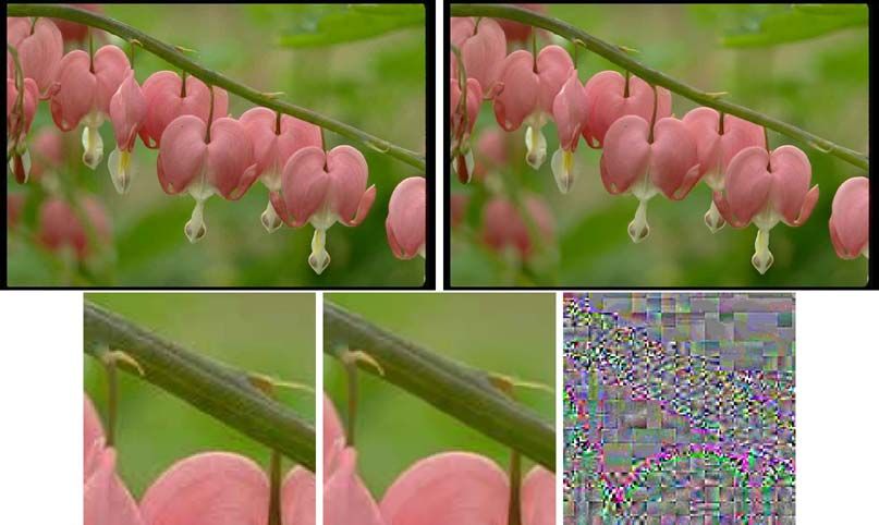
Fig. 13 Lena method noise (in
color) by the sigma filter and the
NL-means. The results of
neighborhood filters improve
dramatically on color images
because similar pixels are much
better identifiable with three
components
Gaussian Convolution The convolution with a Gauss ker- interval (n(i) − h, n(i) + h). The filtered value is therefore
nel Gh is equivalent to the product in the Fourier domain a deterministic function of n(i) and h. Independent random
with a Gauss kernel of inverse standard deviation G1/ h . variables are mapped by a deterministic function on inde-
Therefore, convolving the noise with a kernel reinforces the pendent variables. Thus the noise to noise requirement is as-
low frequencies and cancels the high ones. Thus, the filtered ymptotically satisfied by the bilateral filter. A visual check
noise will no more be a white noise and actually shows big in Fig. 15 fully confirms this theoretical result.
grains due to its prominent low frequencies.
NL-Means Algorithm Figure 15 indicates that NL-means
Total Variation Minimization The Fourier transforms of satisfies the noise to noise principle in the same extent as a
the total variation minimization and the Gaussian filtering classical bilateral filter. However, a mathematical statement
are quite similar even if the total variation preserves some and proof of this property are intricate and we shall skip
high frequency components. them.
Wavelet Thresholding Noise filtered by a wavelet thresh- 4.3 Statistical Optimality
olding is no more a white noise. The few coefficients with
a magnitude larger than the threshold are spread all over The statistical optimality means the ability of a generalized
the image. The pixels which do not belong to the support neighborhood filter to find the right set of pixels J (i) for
of one of these coefficients are set to zero. The visual result performing the average yielding the new estimate for u(i).
is a constant image with superposed wavelets as displayed in This principle for the comparison of denoising algorithms
Fig. 14. It is easy to prove that the denoised noise is spatially applies for all algorithms performing an average over a set
highly correlated. of selected pixels, namely, all neighborhood filters including
NL-means and all motion compensated movie denoising al-
Bilateral Filter For simplicity consider the case where the gorithms (AWA, LMMSE, . . .).
grey level neighborhood is an interval. Given a noise realiza-
tion, the filtered value by the bilateral filter at a pixel i only Principle 3 A generalized neighborhood filter is optimal if
depends on its value n(i) and the parameters h and ρ. The it finds for each pixel i all and only the pixels j having the
bilateral filter averages noise values at a distance from n(i) same model as i.
less or equal than h. Thus as the size ρ of the neighborhood
increases by the law of large numbers the filtered value tends Returning to the signal dependent noise model given by
to the expectation of the Gauss distribution restricted to the Hypothesis 1, we notice that the ideal denoising algorithmInt J Comput Vis (2008) 76: 123–139 135 Fig. 14 Noise to noise principle: Application of the denoising algorithms to a noise sample. From left to right and top to bottom: noise sample (σ = 15), filtered noise by the Gaussian filtering, total variation minimization, hard wavelet thresholding, bilateral filter and the NL-means algorithm. The parameters of each algorithm have been tuned in order to have a filtered noise of standard deviation 2.5. For the neighborhood or bilateral filter the research zone has been fixed to 21 × 21 and for NL-means we have used the whole image. Therefore, only the h parameter has been tuned in order to obtain the desired standard deviation Fig. 15 Noise to Noise principle: Fourier transforms of the filtered noises displayed in Fig. 14. The Fourier transform of a Gaussian white noise is a Gaussian white noise from that point of view would give for J (i) the set of all pix- As displayed in Fig. 16, the orientation computed by the els j with the same original, noiseless value Φ(j ) = Φ(i) anisotropic filter is not exactly the expected one. This fact as i. This aim is not attainable and can be replaced by a is due to the noise interference on the gradient computation. search for pixels j which are likely to have the same value The noise also degrades the probability distribution of the bi- as i. In movies, by the Lambertian assumption, it can be as- lateral filter. The window comparison of NL-means is more sumed that a non occluded pixel keeps the same grey level robust to noise and yields a more adapted weight configura- in several frames. Thus in motion compensated movie fil- tion. In the wall example of Fig. 16 NL-means does not find ters, J (i) is the trajectory of i. In the case of NL-means, picks the pixels with a similar grey level value while the it is assumed that pixels having similar neighborhoods for classical neighborhood does. This avoids mistakes when the some distance also have close colors. Principle 3 cannot be standard deviation of the noise is increased as displayed in checked in theory but can be in practice explored by dis- Fig. 17. NL-means shows a good ability for the restoration playing the probability distribution of w(j ), j ∈ J (i) for of binary textures without assuming any prior about the tex- various algorithms and images. In that way it can be checked ture statistics. When this prior is available optimal solutions whether J (i) corresponds to the pixels j perceptually equiv- can be obtained by imposing the statistical constraints as re- alent or similar to i. This visualization is actually quite in- cently proposed in Cremers and Grady (2006) via a graph formative as illustrated in Figs. 16 and 18. cuts algorithm.
136                                                                                                                  Int J Comput Vis (2008) 76: 123–139

Fig. 16 Weight distribution of NL-means, the bilateral filter and the anisotropic filter used to estimate the central pixel in four detail images

Fig. 17 Denoising experiment
on a noisy periodic texture.
From top to bottom and left to
right: noisy image (standard
deviation 35), total variation
minimization, translation
invariant hard thresholding
(threshold 3σ ), translation
invariant hard thresholding
                     √
(optimal threshold 2 log Nσ ),
bilateral filter and NL-means

4.3.1 Statistical Optimality and the Aperture Problem                        The algorithm favors pixels with a similar local configura-
                                                                             tion even if they are far away from the reference pixel. As
Let us now address the problem of statistical optimality for                 the similar configurations move, so do the weights. Thus,
movies. We shall sustain the position that, in fact, motion                  the algorithm is able to follow the similar configurations
estimation is not only unnecessary, but probably counter-                    when they move without any explicit motion computation.
productive. The aperture problem, viewed as a general phe-                   No need to solve any aperture problem. This problem turns
nomenon in movies, can be positively interpreted in the fol-                 out to be a help for denoising purposes.
lowing way: There are many pixels in the next or previous
frames which can match the current pixel. Thus, it seems
sound to use not just one trajectory, but rather all similar                 5 NL-means vs Classical Neighborhood Filters.
pixels to the current pixel across time and space.                             A Simple Example
    Motion estimation algorithms try to solve the aperture
problem. The block matching algorithm chooses the pixel                      In this section we shall discuss more extensively the applica-
with the more similar configuration, thus loosing many other                 tion of the neighborhood filters to a simple piece-wise con-
interesting possibilities, as displayed in Fig. 8. Algorithms                stant image as the one displayed in Fig. 19. The analysis of
based on the optical flow constraint must impose a regular-                  this image can be decomposed in two parts depending if the
ity condition of the flow field in order to choose a single tra-             research window contains the edge or it is totally flat. For
jectory. Thus, the motion estimation algorithms are forced to                this analysis we shall use a simplified version of the NL-
choose a candidate among all possible equally good choices.                  means and neighborhood filter, that is,
However, when dealing with sequence restoration, the re-
dundancy is not a problem but an advantage. Figure 8 shows                                       1
                                                                             NLh,n u(i) =                          u(j ),
all possible and equally good candidates for the averaging.                                   |J (i)|
                                                                                                        j ∈J (i)
Why not take all of them.
    Figure 18 displays the probability distribution of the                   where J (i) = {j ∈ R(i) | dn (i, j ) ≤ h}, R(i) denotes a re-
weights computed by NL-means for three different cases.                      search zone around the interest pixel and dn (i, j ) denotes the
Int J Comput Vis (2008) 76: 123–139 137
Fig. 18 Weight distribution of
NL-means applied to a movie.
In (a), (b) and (c) the first row
shows a five frames image
sequence. In the second row, the
weight distribution used to
estimate the central pixel (in
white) of the middle frame is
shown. The weights are equally
distributed over the successive
frames, including the current
one. They actually involve all
the candidates for the motion
estimation instead of picking
just one per frame. The aperture
problem can be taken advantage
of for a better denoising
performance by involving more
pixels in the average
Fig. 19 Comparison of neighborhood filters and NL-means on a piecewise constant image. From left to right: input image, NL-means filtered
image and the neighborhood filter with an increasing value of h. Using the whole image as research zone, NL-means is able to recover the original
image almost perfectly with h = 2σ 2 . For the neighborhood filter we have used a research zone of 7 × 7 pixels. For h small the neighborhood filter
is not able to reduce much noise and by increasing the value of h we begin to filter excessively the edge. In contrast with the neighborhood filter,
NL-means is able to reduce the noise with a very conservative value of the filtering parameter
squared normalized Euclidean distance between two com- of the algorithm to a noise sample and the committed error
parison windows around i and j of size n. just as the noise reduction.
As we discussed in Sect. 4.2, the filtered noise value of
5.1 A Research Zone Totally Contained Inside the Same
the neighborhood filter does not depend on the size of the
Region
research window but only on the value of h. This means
In that case, the original grey level value of the considered that in order to decrease the error inside flat zones we must
pixels is the same. This case can be viewed as the application increase the value of h as illustrated in Fig. 19. As we use138 Int J Comput Vis (2008) 76: 123–139
√ √ √
the same value for all the image this fact becomes critical where mi / 2σ and ni / 2σ follow a N (c/ 2σ, 1) and
when we get near any edge or detail. N (0, 1) distributions, respectively, and W denotes the num-
The use of a comparison window by NL-means permits ber of pixels with a different grey level value inside the com-
a higher noise reduction while keeping a small value of h. parison window. The distribution of the above distances fol-
We begin by studying the difference between two noise win- lows a non central
√ chi squared distribution of parameters n
dows of size n. If we denote by dn the normalized squared and λ = W ∗ ( 2σ )2 .
Euclidean distance, then The above normalized distance has mean 1 + (W/n)λ2
and variance n2 (1 + 2λ2 (W/n)). Therefore, the distance be-
2
dn 1 mi tween two windows completely contained in different sides
= √
2σ 2 n 2σ of the edge has a mean 1 + λ2 and a variance n2 (1 + 2λ2 ).
i
The mean is independent of n while the variance tends to
√ zero as n increases. Thus, windows from the same side of
where mi / 2σ follows a N (0, 1) and then ndn /2σ 2 follows
the edge can be better separated from the incorrect ones as
a χ -squared distribution with n degrees of freedom.
n increases. The same argument applies when the ratio W/n
For a sake of simplicity in the mathematical calculations,
is kept constant while n increases. For the neighborhood fil-
we assume that the central point of the window is not used in
ter (n = 1), the above statistics shows that the comparison of
the comparisons. In that case independent values are being
one single pixel is not robust enough. Indeed, the standard
averaged and the next theorem estimates the achieved noise
deviation of the distance of two pixels on different sides of
reduction.
the edge is larger than the distance between the mean dis-
tances of the correct and incorrect choices.
Theorem 1 Assume that the n(i) are i.i.d. with zero mean
and variance σ 2 . Then, the filtered noise by the NL-means
algorithm NLh,n satisfies, 6 Conclusion
1
VarNLh,n n(i) = σ 2, A common framework for the study of the neighborhood fil-
βn ( 2σh 2 )|R(i)| ters has been presented. We have proposed three principles
for the comparison of denoising methods evaluating the loss
where
of image structure, the creation of artifacts, and the com-
nx plete usage of image self-similarity. After a structural com-
βn (x) = fχn2 (y)dy, parison of non-local denoising methods with other classes,
−∞
we have shown that movie denoising can avoid the explicit
and fχn2 denotes the probability distribution function of computation of an optical flow estimate. What is left to be
a χn2 . done? The very recent extensions of NL-means we men-
tioned in the introduction point towards the involvement of
This result shows that we can increase the noise reduction still more sophisticated statistical instruments. Beyond de-
by increasing the size of the sample and keeping the same noising, we have seen that the association with each pixel
value of h as illustrated in Fig. 19. We can for example set a of a probability distribution weighting its similarity with the
conservative threshold h = 2σ 2 and have a noise reduction other pixels of the image may become a central tool in image
2
tending to |R(i)| as n increases. analysis. This rich structure unfolds image information and
should be used for algorithm which simultaneously analyze
and process images. The recent work of Gilboa and Osher
5.2 A Research Zone Containing the Edge
(2006) points towards this direction. These authors use NL-
means as a segmentation tool.
In this case, the risk is to average pixels with an original
value different from the pixel of interest. Therefore, we want Acknowledgements The first two authors were supported by the
to separate as much as possible the distances from the cor- Ministerio de Ciencia y Tecnologia under grant MTM2005-08567.
rect pixels from the distances of the incorrect ones. Follow-
ing the same notations of the above section and denoting by
c the contrast between the two different regions of the im- References
age, we can write the distance between two windows as
Alvarez, L., Guichard, F., Lions, P. L., & Morel, J. M. (1993). Axioms
W 2 n and fundamental equations of image processing. Archive for Ra-
dn 1 mi ni 2 tional Mechanics and Analysis, 123, 199–257.
= √ + √ , Attneave, F. (1954). Some informational aspects of visual perception.
2σ 2 n 2σ 2σ
i=0 j =W +1 Psychological Review, 61, 183–193.You can also read