Reproducing complex simulations of economic impacts of climate change with lower-cost emulators - GMD
←
→
Page content transcription
If your browser does not render page correctly, please read the page content below
Geosci. Model Dev., 14, 3121–3140, 2021
https://doi.org/10.5194/gmd-14-3121-2021
© Author(s) 2021. This work is distributed under
the Creative Commons Attribution 4.0 License.

Reproducing complex simulations of economic impacts of climate
change with lower-cost emulators
Jun’ya Takakura1 , Shinichiro Fujimori2 , Kiyoshi Takahashi1 , Naota Hanasaki3 , Tomoko Hasegawa4 ,
Yukiko Hirabayashi5 , Yasushi Honda6 , Toshichika Iizumi7 , Chan Park8 , Makoto Tamura9 , and Yasuaki Hijioka3
1 Social  Systems Division, National Institute for Environmental Studies, Tsukuba, 305-8506, Japan
2 Department    Environmental Engineering, Kyoto University, Kyoto, 615-8540, Japan
3 Center for Climate Change Adaptation, National Institute for Environmental Studies, Tsukuba, 305-8506, Japan
4 Department of Civil and Environmental Engineering, Ritsumeikan University, Kusatsu, 525-8577, Japan
5 Department of Civil Engineering, Shibaura Institute of Technology, Tokyo, 135-8548, Japan
6 Faculty of Health and Sport Sciences, University of Tsukuba, Tsukuba, 305-8577, Japan
7 Institute for Agro-Environmental Sciences, National Agriculture and Food Research Organization, Tsukuba, 305-8604 Japan
8 Department of Landscape Architecture, College of Urban Science, University of Seoul, Seoul, 02504, Korea
9 Global and Local Environment Co-creation Institute, Ibaraki University, Mito, 310-8512, Japan

Correspondence: Jun’ya Takakura (takakura.junya@nies.go.jp)

Received: 16 October 2020 – Discussion started: 20 November 2020
Revised: 16 April 2021 – Accepted: 26 April 2021 – Published: 1 June 2021

Abstract. Process-based models are powerful tools for sim-       1   Introduction
ulating the economic impacts of climate change, but they
are computationally expensive. In order to project climate-
change impacts under various scenarios, produce probabilis-      Climate change has diverse impacts on society and a wide
tic ensembles, conduct online coupled simulations, or ex-        range of sectors (IPCC, 2014), and these impacts should be
plore pathways by numerical optimization, the computa-           quantitatively evaluated to manage overall risks. If we can
tional and implementation cost of economic impact calcula-       monetize these impacts, a variety of risks across different
tions should be reduced. To do so, in this study, we developed   sectors and regions can be considered on a unified scale.
various emulators that mimic the behaviours of simulation        This information helps us to design climate-change-related
models, namely economic models coupled with bio/physical-        policies. It also contributes to estimating the social cost of
process-based impact models, by statistical regression tech-     carbon.
niques. Their performance was evaluated for multiple sec-           There are a variety of ways to estimate the economic im-
tors and regions. Among the tested emulators, those com-         pacts of climate change (Tol, 2002; Stern, 2006; Ciscar et al.,
posed of artificial neural networks, which can incorporate       2011; Burke et al., 2015; Takakura et al., 2019). Among the
non-linearities and interactions between variables, performed    existing approaches, process-based bio/physical impact mod-
better particularly when finer input variables were available.   els coupled with an economic model are widely used, and
Although simple functional forms were effective for approxi-     they tend to be elaborate and complex (Weyant, 2017; Diaz
mating general tendencies, complex emulators are necessary       and Moore, 2017). Since these process-based simulations
if the focus is regional or sectoral heterogeneity. Since the    can represent underlying bio/physical or economic processes
computational cost of the developed emulators is sufficiently    explicitly based on the governing equations, their applica-
small, they could be used to explore future scenarios related    tions are not limited to prediction of the outcome variables.
to climate-change policies. The findings of this study could     Process-based simulations can also contribute to deeper un-
also help researchers design their own emulators in different    derstanding of the focal phenomena, and they can simulate
situations.                                                      outcomes under purely counterfactual conditions that never
                                                                 occurred in the past. This cannot be achieved by simpler

Published by Copernicus Publications on behalf of the European Geosciences Union.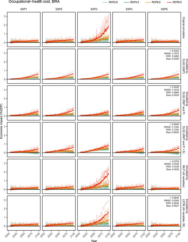
3122                         J. Takakura et al.: Reproducing complex simulations of economic impacts of climate change

macroscopic methods (e.g. Burke et al., 2015). Despite these       and Sterner, 2017). In this case, the impact of climate change
advantages, it is not always easy for researchers to handle        is expressed by a quadratic function of the mean tempera-
these elaborate process-based models (particularly for model       ture rise (such simple damage functions are not called emu-
users, rather than model developers) because of the model-         lators in general, but they act in the same way as the so-called
specific knowledge, skills, and input data that are required.      emulators). It is also possible for simple damage functions
This is especially the case when multiple sectors are targeted     to incorporate socioeconomic conditions. Compared to the
because completely different impact models are developed           simple damage functions, typical climate-change impact em-
for each sector.                                                   ulators adopt relatively complex functional forms. These in-
   The high computational cost of process-based impact sim-        clude multivariate regression or statistical machine learning
ulations is another problem, and this also makes online cou-       techniques such as an artificial neural network (ANN; Harri-
pling with other models difficult. Online coupling of impact       son et al., 2013; Oyebamiji et al., 2015; Schnorbus and Can-
models is required, for example, to represent feedback ef-         non, 2014). By using these techniques, emulators can repre-
fects of climate-change impacts on climate-change mitiga-          sent more complex input–output relationships, but existing
tion (Matsumoto, 2019) and many other synergies and trade-         studies using these techniques mainly focus on bio/physical
offs among sectors (Yokohata et al., 2020). The possibility of     impacts rather than economic impacts of climate change. In
simulation under various scenarios or probabilistic ensemble       our previous work, it has been demonstrated that the simu-
simulation of impacts also depends on the computational cost       lated economic impacts of climate change are affected by so-
of the impact simulations. Mainly due to their high compu-         cioeconomic conditions as well as the climate conditions and
tational cost, typically, process-based simulations of the im-     that there are complex, non-linear interactions (Takakura et
pacts can be conducted under a limited number of scenar-           al., 2019). Therefore, using such advanced techniques can be
ios, such as representative concentration pathways (RCPs)          beneficial to emulations of the economic impacts of climate
(van Vuuren et al., 2011). While these scenarios reasonably        change, too.
cover the plausible range of the radiative forcing levels at the      Besides the choice of functional form, there are multiple
end of the 21st century, there are an infinite number of emis-     options in the selection of the input variables. By leveraging
sion pathways which are not included in the discrete RCP           all the information used in the simulation and using suffi-
scenarios (e.g. intermediate pathway between RCP2.6 and            ciently complex models, it is theoretically possible to per-
RCP4.5). Recently, particularly after the Paris Agreement,         fectly reproduce the results of the simulation by the em-
more attention has been paid to the effect of subtler differ-      ulation (Cybenko, 1989). On the other hand, in practical
ences in emission pathways (Keywan et al., 2021). When we          terms, the number of parameters used in the emulation model
try to find the optimal pathway by numerical optimization,         will increase, and it is impossible to identify the parameters
repetitive calculations of the objective function which we         based on the limited simulation results. Therefore, we use
want to minimize or maximize are needed, and if the impacts        some representative variables as the input to the emulators
of climate change are included in the objective function, they     by summarizing the original input data. These input variables
also need to be calculated many times until the value of the       should contain information on climate conditions and socioe-
objective function converges. Ensemble simulation of the im-       conomic conditions, and those jointly determine the magni-
pacts is also important to manage the risk because of the          tude of the economic impacts of climate change. What kind
probabilistic characteristics of the climate (Mitchell et al.,     of information is important may depend on what kind of im-
2017; Mizuta et al., 2017), but this also requires a large num-    pacts we focus on. For example, some impacts can be accu-
ber of simulation runs.                                            rately predicted by changes in temperature, but others may
   Therefore, reducing the implementation and computa-             depend more on changes in precipitation or socioeconomic
tional costs of impact calculations is useful for many pur-        conditions.
poses even if representation of the underlying processes is           To better design emulators, we need to identify impor-
omitted when the focus is on the outcome variable, not on          tant factors which affect performance, i.e. those that deter-
these underlying processes.                                        mine how well the emulators can reproduce the results of
   One possible way to solve these issues is statistically mim-    simulations. However, there have been no systematic com-
icking the behaviours of the process-based impact simula-          parisons of the attained performance of the emulators con-
tions. Such approaches are called emulations (Castelletti et       sidering the above-mentioned factors. The purpose of this
al., 2012). In emulations, emulators try to reproduce the rela-    study was to develop and evaluate emulators for the projec-
tionships between the inputs and outputs of the impact mod-        tion of the economic impacts of climate change and identify
els regarding the underlying processes as a black box. A sim-      the relationship between the attained performance of emula-
ple but widely used way involves expressing the impact by a        tors and functional forms or input variables. For this purpose,
simple damage function. Such simplification is adopted in          we used the results of economic impact simulations covering
several integrated assessment modelling frameworks (Wald-          many sectors (Takakura et al., 2019). In this study, the re-
hoff et al., 2014; Nordhaus, 2017). The most typical form          sults of the original simulation results were regarded as the
of such a damage function is a quadratic function (Howard          “ground truth”, and emulators tried to reproduce the ground

Geosci. Model Dev., 14, 3121–3140, 2021                                            https://doi.org/10.5194/gmd-14-3121-2021
J. Takakura et al.: Reproducing complex simulations of economic impacts of climate change                                                                 3123

truth statistically when corresponding input was given. Var-     Table 1. List of modelled sectors. In principle, the results of simu-
ious emulators (different functional forms and input vari-       lations obtained in Takakura et al. (2019) were used.
ables) were developed, and their performance, how well they
can reproduce the results of simulations, was systematically           Simulated economic impact                       Way of monetization
compared.                                                              Agricultural productivitya                      CGE model
   We expect there are two main groups of readers of this              Undernourishment                                CGE model + VSL
article. The first group is those who wish to use the emula-           Heat-related excess mortality                   VSL
                                                                       Cooling/heating demand                          CGE model
tors developed herein. The second group is the readers who             Occupational-health cost                        CGE model
wish to develop their own emulators using their simulation             Hydropower generation capacity                  CGE model
results. We provide specific information on our development            Thermal power generation capacity               CGE model
process. This information could be particularly useful for the         Fluvial flooding                                Economic damage function
second group. For the first group, the emulators we have de-           Coastal inundationb                             Economic damage function
                                                                   a Definition of the baseline (no-climate-change condition) was changed slightly
veloped can be freely downloaded from a repository (details        compared to that of the original study. b Original results imputed by emulation-like
below) and explored in conjunction with this article to avoid      technique due to data unavailability.
any potential issues in terms of misuse or misinterpretation.

                                                                 The simulations were conducted sector by sector, and inter-
2     Materials and methods                                      actions among sectors were not considered. More details on
                                                                 the original process-based economic impact simulations are
2.1    Simulation of the economic impacts of climate             described in Takakura et al. (2019) and in Sect. S1 in the
       change                                                    Supplement.
                                                                    The simulations were conducted under the shared socioe-
We used previously published results of simulations, in          conomic pathways–representative concentration pathways
which up to nine different sectoral economic impacts of cli-     (SSP–RCP) scenario matrix (van Vuuren et al., 2013). We
mate change were simulated by bio/physical impact models         used five SSPs (SSP1, SSP2, SSP3, SSP4, and SSP5) and
coupled with economic models (Takakura et al., 2019). Here,      four RCPs (RCP2.6, RCP4.5, RCP6.0, and RCP8.5). More-
“economic models” refers to the methodologies by which           over, in order to incorporate the uncertainty in climate projec-
bio/physical impacts are monetized regardless of their ways      tions, we used five different global climate models (GCMs),
of monetization. We used the simulated economic impacts          namely, HadGEM2-ES, IPSL-CM5A-LR, MIROC-ESM-
caused by changes in agricultural productivity (Iizumi et al.,   CHEM, GFDL-ESM2M, and NorESM1-M (Hempel et al.,
2017; Fujimori et al., 2018), undernourishment (Hasegawa         2013). Therefore, there are 100 (5 × 4 × 5) scenario runs in
et al., 2016a), heat-related excess mortality (Honda et al.,     total. The computational general equilibrium model covers
2014), cooling/heating demand (Hasegawa et al., 2016b;           17 regions (AIM’s 17 regions shown in Table S1 in the Sup-
Park et al., 2018), occupational-health cost (Takakura et al.,   plement), and thus we have economic impacts for these 17
2017), hydropower generation capacity (Zhou et al., 2018b),      regions (for sectors whose economic impacts can be simu-
thermal power generation capacity (Zhou et al., 2018a, c),       lated for each country, the results were aggregated for the 17
fluvial flooding (Kinoshita et al., 2018), and coastal inunda-   regions).
tion (Tamura et al., 2019) due to climate change. In each sec-      While it is impossible to evaluate how accurate these sim-
tor, bio/physical impacts were modelled by specific process-     ulation results are because of inherent uncertainty in the sim-
based impact models, and then the impacts were monetized         ulations, we regard these simulation results as the ground
either by multiplying values of statistical life (VSL) (OECD,    truth. We used the results of these simulations to construct
2012) by the damage functions which translate bio/physical       and evaluate the emulators.
impacts into economic damages (Kinoshita et al., 2018;
Tamura et al., 2019) or by a computational general equi-         2.2      Overall framework of the emulations
librium (CGE) model (Fujimori et al., 2012, 2017). Here,
the CGE model is the AIM/Hub model (formerly known               Figure 1 shows the framework of the simulation and the em-
as the AIM/CGE model) (Table 1). While the simulations           ulation of the economic impacts of climate change. By using
were conducted under a unified climatic and socioeconomic        the emulators, we want to get results as similar as possible
scenario framework and target years, they differ conceptu-       to the results of process-based simulations when the input
ally depending on characteristics of the impacts and the ca-     data or scenario is given. While emulators do not explicitly
pability of the models. For example, some simulations in-        model the underlying phenomena, they do have parameters,
tend to capture year-by-year fluctuations in impacts, while      and by tuning these parameters, they can statistically mimic
others focus only on longer-term impacts. Further, some-         the behaviours (input–output relationship) of simulations.
times pure process-based models were not used, and statisti-        Here, ys,r,t|sc denotes the simulated economic impact (in
cal regression-based methods were also used in hybrid ways.      percentage of GDP) in sector s, in region r, in year t, and un-

https://doi.org/10.5194/gmd-14-3121-2021                                                    Geosci. Model Dev., 14, 3121–3140, 2021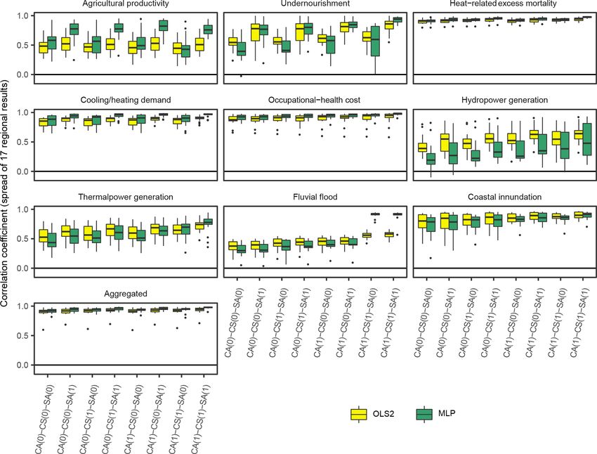
3124                            J. Takakura et al.: Reproducing complex simulations of economic impacts of climate change

Figure 1. Overall framework of simulation and emulation of economic impacts of climate change. Simulated and emulated economic impacts
in sector s, region r, and year t under a scenario sc are denoted as ys,r,t|sc and ŷs,r,t|sc , respectively. The parameters of the emulator are
determined based on the simulated economic impact (represented by the green dash–dot–dash arrow).

der a given scenario sc, and ŷs,r,t|sc is the corresponding em-          perceptron (MLP), and a recurrent neural network composed
ulated economic impact. A scenario sc comprises the com-                  of long short-term memory units (LSTM). For the sake of
bination of SSP, RCP, and GCM. The emulated economic                      simplicity, we omit the suffixes s, r, and sc in this section,
impact ŷs,r,t|sc is calculated by the function fs,r (·) receiving        and the ith variable in vector x t is denoted as xt,i .
the input x r,t|sc as expressed in Eq. (1).                                   OLS1 is the simplest form of the emulator, expressed as
                                                                         Eq. (2).
ŷs,r,t|sc = fs,r x r,t|sc                                     (1)                   X
                                                                          ŷt = a0 +    ai xt,i                                      (2)
The emulator (function fs,r (·)) is constructed for each sec-                           i
tor and region. The input x r,t|sc is the (vector of) variable(s)
which is used to emulate the economic impact in region r in               OLS2 includes squared terms and thus can express some cur-
year t under a given scenario sc. One important characteristic            vature in the response.
of the input x r,t|sc is that there is no suffix s. This means that                  X              X
                                                                                                          2
                                                                          ŷt = a0 +     a1i xt,i +  a2i xt,i                    (3)
the input variable is not sector-specific and common input
                                                                                        i             i
data can be used across sectors.
                                                                          OLS2i has product terms as well as squared terms, and it can
2.3     Tested emulators                                                  represent some types of interactions among variables.
                                                                                     X            X            X
2.3.1    Functional forms                                                 ŷt = a0 +   a1i xt,i +        2
                                                                                                    a2i xt,i +   aij xt,i xt,j     (4)
                                                                                        i             i            i6=j
We tested a variety of emulators (different functional forms
and input variables) ranging from very parsimonious to com-               Simple regressions such as these are widely used, but their
plex alternatives. For the functional forms, we used ordinary             capability to express complex phenomena is limited. Cur-
least squares regression (OLS1), ordinary least squares re-               rently, more elaborate methods based on statistical machine
gression with square terms (OLS2), ordinary least squares re-             learning techniques such as ANNs are available. Thus, to rep-
gression with square and product terms (OLS2i), multi-layer               resent more complex non-linearities and interactions among

Geosci. Model Dev., 14, 3121–3140, 2021                                                      https://doi.org/10.5194/gmd-14-3121-2021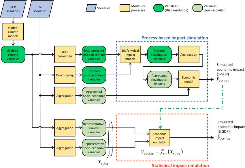
J. Takakura et al.: Reproducing complex simulations of economic impacts of climate change                                    3125

variables, we also applied ANN-based techniques to the em-         tation as follows.
ulations. MLP is a traditional, but effective and widely used,
                                                                               P
ANN-based technique that can be applied to the purpose of                           g,d wg tt|sc (g, d)
regression and thus to the emulation. LSTM is also an ANN-         agtt|sc =               P                                   (8)
                                                                                   |Dt |        g wg
based technique designed to handle time-series data and can                       P
represent time-dependent characteristics of the data (e.g. cu-                       g∈rs,d wg tt|sc (g, d)
                                                                   artrs,t|sc =                 P                              (9)
mulative effects in the economic impacts) as well as non-                               |Dt |       g∈rs wg
linearities and interactions among variables. Thus, it may                        P
                                                                                      g∈rs,d wg pt|sc (g, d)
better act as the emulator if time-series data are available as    arprs,t|sc =                 P                             (10)
the input. While their strict mathematical formulations are                          |Dt |           g∈rs wg
                                                                                    P
lengthy, MLP can be expressed as                                                         g∈rs,d∈q wg tt|sc (g, d)
                                                                   qrtq,rs,t|sc =                    P                        (11)
                                                                                           Dq,t          g∈rs wg
                                                                                     P
ŷt = f (x t , W ) ,                                        (5)                          g∈rs,d∈q wg pt|sc (g, d)
                                                                   qrpq,rs,t|sc =                     P                       (12)
                                                                                            Dq,t          g∈rs wg

where W is the weights (parameters) of the model. LSTM             Here, |Dt | is the number of days in year t, and |Dq,t |
has time-dependent internal state s t , and the output and the     is the number of days belonging to quarter of a year q.
internal state at time t can be expressed as                       Quarters are grouped following the calendar year, namely,
                                                                   January–February–March, April–May–June, July–August–
                                                                   September, and October–November–December. Coefficient
ŷt = f (s t−1 , x t , W ) ,                                (6)    wg is a weight which is proportional to the area of the grid
s t = g (s t−1 , x t , W ) .                                (7)    g. Regions are indicated by the subscript rs. Note that rs is
                                                                   based on the classification of SREX’s 26 regions defined in
                                                                   IPCC (2012) and different from r (Table S2 in the Supple-
See, for example, Goodfellow et al. (2016) for details on          ment). While our interest is estimating the economic impacts
MLP and LSTM. Hyperparameters in the ANN-based mod-                in each of AIM’s 17 regions represented by r, each such re-
els were determined based on preliminary examinations. The         gion contains different climate zones because r is classified
number of hidden layers and the number of units in each            from the viewpoint of economic modelling rather than cli-
layer were set to 2 and 32, respectively, and the early-           matic and geographic conditions. Thus, to incorporate het-
stopping technique was used to avoid overfitting of the mod-       erogeneity in climate conditions within an AIM region, we
els.                                                               use rs instead of r to define climate variables.
                                                                      For socioeconomic variables, values are based on the SSP
2.3.2    Input variables                                           scenarios (Kc and Lutz, 2017; Dellink et al., 2017). Based on
                                                                   the population (popt|sc (c)) and GDP (gdpt|sc (c)) in country
                                                                   c in year t under a given scenario sc, regional population,
When inputting climate conditions into the emulators, the          GDP, and GDP per capita are calculated as follows. GDP is
dimension of the data should be reduced. One typical way           measured in USD (2005) based on the market exchange rate.
to do this is to spatially and temporally aggregate the high-
resolution original data. For climate data, the most parsimo-                     X
nious choice involves using the global mean temperature, but       popr,t|sc =          popt|sc (c)                           (13)
                                                                                  c∈r
this method cannot represent regional and seasonal charac-                        X
teristics of climate conditions. Precipitation also plays an im-   gdpr,t|sc =     gdpt|sc (c)                                (14)
                                                                                  c∈r
portant role for some specific sectors (e.g. hydropower gener-
ation capacity, fluvial flooding). We prepared several kinds of    gpcr,t|sc = gdpr,t|sc /popr,t|sc                           (15)
input data with different spatial and temporal resolutions by
aggregating daily gridded near surface temperature and pre-        When inputting variables to the emulators, it is desirable that
cipitation data generated by GCMs in CMIP5 (Taylor et al.,         their values be within a limited range to ensure the stabil-
2011). First, the spatial resolution of the gridded GCM output     ity of numerical computation. Effects of biases in GCMs
data was downscaled to 0.5 × 0.5◦ by bilinear interpolation.       should also be alleviated. For this purpose, we used the rela-
We denote this downscaled gridded temperature as tt|sc (g, d)      tive changes of these variables as inputs to the emulators. For
and precipitation as pt|sc (g, d), where g denotes grid and d      temperature, changes were defined by the difference from
denotes day of the year. We calculate annual global mean           the base-period (1991–2010) values. For the other variables,
temperature, annual regional mean temperature and precipi-         changes were defined by a log ratio to the base-period or
tation, and quarterly regional mean temperature and precipi-       base-year (2005) values (Table 2).

https://doi.org/10.5194/gmd-14-3121-2021                                                   Geosci. Model Dev., 14, 3121–3140, 2021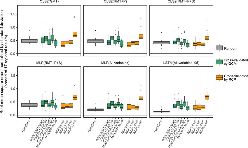
3126                         J. Takakura et al.: Reproducing complex simulations of economic impacts of climate change

Table 2. Candidate input variables. Socioeconomic variables are defined for AIM’s 17 regions, while climatic variables are defined for
SREX’s 26 regions.

                             Variable name    Variable            Spatial resolution   Temporal resolution
                             1agtt|sc         Temperature         Global               Annual
                             1artrs,t|sc      Temperature         SREX 26 regions      Annual
                             1arprs,t|sc      Precipitation       SREX 26 regions      Annual
                             1qrtq,rs,t|sc    Temperature         SREX 26 regions      Quarterly
                             1qrpq,rs,t|sc    Precipitation       SREX 26 regions      Quarterly
                             1popr,t|sc       Population          AIM 17 regions       Annual
                             1gdpr,t|sc       GDP                 AIM 17 regions       Annual
                             1gpcr,t|sc       GDP per capita      AIM 17 regions       Annual

2.4     Comparison                                                     suitable. Thus, we tested OLS2 and MLP using these vari-
                                                                       ables (Table 5).
As explained in Sect. 2.3, we have various types of emulators
(functional forms) and candidate input variables. We con-              2.4.4    Comparison 4
ducted comparisons under selected practically relevant con-
ditions among the possible combinations.                               In the previous comparisons, only simultaneous data were
                                                                       used; that is, when emulating the economic impacts in year
2.4.1    Comparison 1                                                  t, climate and socioeconomic conditions in year t are used.
                                                                       Cumulative or carry-over effects can also exist in the sim-
We quantified the performance of the very simple damage                ulated impacts. Therefore, including climate and socioeco-
functions (OLS1 and OLS2), which only consider the global              nomic conditions in past years as the input to the emulator
mean temperature, and compared the performance when re-                can also contribute to better reproduce the results of the eco-
gional climate conditions were considered (Table 3). Here,             nomic simulation. To evaluate the effects of inclusion of in-
rs(r) represents a set of SREX regions corresponding to an             formation in past years, we tested the performance of arti-
AIM region r (Table S3 in the Supplement).                             ficial neural networks which can consider time-series infor-
                                                                       mation (LSTM) with time-series data of different length (10-
2.4.2    Comparison 2                                                  year data to capture relatively short-period effects and 95-
                                                                       year data which can capture the entire simulation period as
We investigated the effects of considering socioeconomic               shown in Table 6).
conditions. It is also expected that there are interactions be-
tween climate conditions and socioeconomic conditions. To              2.5     Evaluation
identify whether such interactions can be expressed by a sim-
ple method, we included product terms in OLS2i (Table 4).              2.5.1    Evaluation procedure metrics

2.4.3    Comparison 3                                                  Parameters in the emulators are optimized based on the sim-
                                                                       ulation results. If, however, we simply optimized these pa-
In comparisons 1 and 2, relatively simple functional forms             rameters based on the existing data (simulation results) and
and temporally coarsely aggregated (annual) climate vari-              evaluated them by the same data, the performance of the em-
ables are used. Such an aggregation possibly causes loss of            ulators might be overestimated compared to the situation in
information. For example, crop models consider crop calen-             which new data are input to the emulators. This phenomenon
dars, and thus the temperature changes in growing and non-             is known as overfitting or overlearning. To avoid the ef-
growing seasons have different effects on their original simu-         fects of overfitting, we use the cross-validation strategy. We
lation results. Regarding the economic impacts, climatic and           have simulation results for 100 scenarios (5 SSPs×4 RCPs×
socioeconomic conditions of the non-target regions can also            5 GCMs), and each scenario has 95 (2006–2100) data points.
affect the target region through, for example, trade in the            We divide the 100 scenario results into 4 groups randomly.
international market, which is simulated by the AIM/Hub                Three-quarters of the data were used to optimize parameters
model. To investigate these possibilities, seasonal climate            in the emulators (training), and prediction values were ob-
variables, climate variables of non-target regions, and socioe-        tained for the remaining one-quarter of the data (test). This
conomic variables of non-target regions were included as in-           procedure was repeated four times by changing the training
put variables. Moreover, when the number of input variables            and test data, and then we got the results of emulation for all
becomes large, more complex functional forms may be more               scenarios. That is, 4-fold cross-validation was performed.

Geosci. Model Dev., 14, 3121–3140, 2021                                                 https://doi.org/10.5194/gmd-14-3121-2021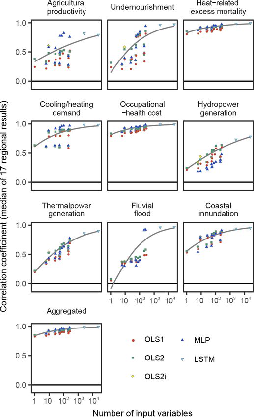
J. Takakura et al.: Reproducing complex simulations of economic impacts of climate change                                                         3127

Table 3. Models and input variables in comparison 1. Input variables are used to emulate the economic impact in year t1 in region r1 for
each sector.

                                  Emulator        Input variables
                                  OLS1/OLS2       x r,t|sc =
                                                             agtt|sc     n           o    t = t1

                                  OLS1/OLS2       x r,t|sc = artrs,t|sc , arprs,t|sc       t = t1 , rs ∈ rs(r1 )

Table 4. Models and input variables in comparison 2. Input variables are variables used to emulate the economic impact in year t1 in region
r1 for each sector.

         Emulator          Input variables
                                                    n           o
         OLS2/OLS2i        x r1 ,t1 |sc = artrs,t|sc , arprs,t|sc                                            t = t1 , rs ∈ rs(r1 )
                                                    n           o n        o n         o n          o
         OLS2/OLS2i        x r1 ,t1 |sc = artrs,t|sc , arprs,t|sc , popr,t|sc , gdpr,t|sc , gpcr,t|sc        t = t1 , rs ∈ rs(r1 ), r = r1

Table 5. Models and input variables in comparison 3. Input variables are variables used to emulate the economic impact in year t1 in region
r1 for each sector.

     Emulator        Input variables
                                              n          o n         o n         o n          o
     OLS2/MLP        x r1 ,t1 |sc = artrs,t|sc , arprs,t|sc , popr,t|sc , gdpr,t|sc , gpcr,t|sc             t = t1 , rs ∈ rs(r1 ), r = r1
                                              n          o n         o n         o n          o
     OLS2/MLP        x r1 ,t1 |sc = artrs,t|sc , arprs,t|sc , popr,t|sc , gdpr,t|sc , gpcr,t|sc             t = t1 , rs ∈ rs(r1 ), ∀r
                                   n           o n            o n         o n         o n          o
     OLS2/MLP        x r1 ,t1 |sc = qrtq,rs,t|sc , qrpq,rs,t|sc , popr,t|sc , gdpr,t|sc , gpcr,t|sc         t = t1 , rs ∈ rs(r1 ), r = r1 , ∀q
                                   n           o n            o n         o n         o n          o
     OLS2/MLP        x r1 ,t1 |sc = qrtq,rs,t|sc , qrpq,rs,t|sc , popr,t|sc , gdpr,t|sc , gpcr,t|sc         t = t1 , rs ∈ rs(r1 ), ∀r, ∀q
                                              n          o n         o n         o n          o
     OLS2/MLP        x r1 ,t1 |sc = artrs,t|sc , arprs,t|sc , popr,t|sc , gdpr,t|sc , gpcr,t|sc             t = t1 , ∀rs, r = r1
                                              n          o n         o n         o n          o
     OLS2/MLP        x r1 ,t1 |sc = artrs,t|sc , arprs,t|sc , popr,t|sc , gdpr,t|sc , gpcr,t|sc             t = t1 , ∀rs, ∀r
                                   n           o n            o n         o n         o n          o
     OLS2/MLP        x r1 ,t1 |sc = qrtq,rs,t|sc , qrpq,rs,t|sc , popr,t|sc , gdpr,t|sc , gpcr,t|sc         t = t1 , ∀rs, r = r1 , ∀q
                                   n           o n            o n         o n         o n          o
     OLS2/MLP        x r1 ,t1 |sc = qrtq,rs,t|sc , qrpq,rs,t|sc , popr,t|sc , gdpr,t|sc , gpcr,t|sc         t = t1 , ∀rs, ∀r, ∀q

Table 6. Models and input variables in comparison 4. Input variables are used to emulate the economic impact in year t1 in region r1 for
each sector.

      Emulator      Input variables
                                  n           o n            o n         o n         o n          o
      MLP           x r1 ,t1 |sc = qrtq,rs,t|sc , qrpq,rs,t|sc , popr,t|sc , gdpr,t|sc , gpcr,t|sc         t = t1 , ∀rs, ∀r, ∀q
                                  n           o n            o n         o n         o n          o
      LSTM          x r1 ,t1 |sc = qrtq,rs,t|sc , qrpq,rs,t|sc , popr,t|sc , gdpr,t|sc , gpcr,t|sc         t = t1 , . . ., t1 − 9, ∀rs, ∀r, ∀q
                                  n           o n            o n         o n         o n          o
      LSTM          x r1 ,t1 |sc = qrtq,rs,t|sc , qrpq,rs,t|sc , popr,t|sc , gdpr,t|sc , gpcr,t|sc         t = t1 , . . ., t1 − 94, ∀rs, ∀r, ∀q

   In some situations, we want to emulate impacts under                   simulation results of three RCPs (5 SSPs×3 RCPs×5 GCMs)
scenarios which are drastically different from the scenar-                and tested by the results of the remaining one RCP (5 SSPs×
ios which are used to develop (or train) the emulators. In                1 RCPs × 5 GCMs).
order to evaluate the performance of the emulators under                     Optimization of the parameters (training) and prediction
such situations, we also conducted cross-validation by GCM                (test) of OLS-based emulators were conducted using the lm
and RCP. Cross-validation by GCM means that the emu-                      function in R 3.4.3 (R Core Team, 2017). ANN-based emula-
lators are trained by the simulation results of four GCMs                 tors were trained and tested using the Keras library (Chollet,
(5 SSPs × 4 RCPs × 4 GCMs) and tested by the results of the               2015) in Python 3.7.3. The Windows operating system (OS)
remaining one GCM (5 SSPs × 4 RCPs × 1 GCMs). Cross-                      was used in all cases.
validation by RCP mean that the emulators are trained by the

https://doi.org/10.5194/gmd-14-3121-2021                                                       Geosci. Model Dev., 14, 3121–3140, 2021
3128 J. Takakura et al.: Reproducing complex simulations of economic impacts of climate change
2.5.2 Evaluation metrics
The performance of the emulators was evaluated based on
the agreement between the results of the simulations and the
emulations. By a chosen emulator, we obtain the values of
emulated economic impacts ŷs,r,t|sc . We also have the val-
ues of the corresponding original simulated economic im-
pact ys,r,t|sc . We measured the agreement between ŷs,r,t|sc
and ys,r,t|sc by correlation coefficient (r), root mean squared
error (RMSE), ratio of RMSE to standard deviation (RSR),
and systematic error (bias). These metrics were calculated
for each sector and region.
The computational cost of the emulators was assessed by
the number of required input data, the number of parame-
ters in a model, model object size (memory size required to
load a model), prediction time, and training time. This was
measured on a PC (CPU: Intel Core i7–8700K (3.70 GHz,
6 cores/12 threads); RAM: 32 GB; OS: Windows 10 Pro).
While the lm function in R was used for OLS-based emu-
lators in the development, they were transplanted to Python
for the assessment of computational cost. Thus, both OLS-
based emulators and ANN-based emulators were assessed
under equal conditions.
3 Results
Figure 2. Performance of emulations in comparison 1. Correlation
We report results for r in the main text since the three metrics coefficients between simulation results and emulation results are
(r, RMSE, and RSR) varied almost parallelly, and systematic shown. Bars and edges of boxes represent medians and first/third-
errors (biases) were nearly negligible for all conditions. Sum- quantile values among 17 regional results. The ends of the whiskers
marized results beyond r (RMSE, RSR, and bias) are avail- show the minimum and maximum values, while outliers are denoted
able in Tables S4 to S13 in the Supplement, and individual by dots if they exist.
values for all sectors and regions are available as electronic
supplementary material. A higher value of r (i.e. r closer to
1) indicates that results of the emulation are similar to those formance of the emulations (Fig. 3). The impacts of climate
of the simulation when the biases are negligible. The value change are determined not only by hazards (climate condi-
of r also indicates how well the variation in the simulation tions) but also by exposure and vulnerability (socioeconomic
results is reproduced by the emulation (square of r is equal conditions) (IPCC, 2014). Most current-generation simula-
to the coefficient of determination or the proportion of ex- tions of economic impacts, including the simulations used in
plained variance). this study, take socioeconomic aspects into account. Thus, it
Figure 2 is the results of comparison 1. While there is is not surprising that emulators could better reproduce the re-
a large variation in the performance of the emulations for sults of simulations by taking socioeconomic variables into
individual sectors, the performance for the aggregated eco- account. Note that there is very little improvement in the re-
nomic impacts is relatively good on average even if they sults with respect to river flooding impacts. This is mainly be-
only consider global mean temperature rise. This implies that cause the same proportion of the population and GDP distri-
using simple damage functions can be useful to grasp the bution data were used in the simulation of the impacts of flu-
rough picture of economic impacts of climate change. On vial flooding across SSPs due to data availability (Takakura
the other hand, when we focus on more minute components, et al., 2019), and the simulated economic impacts (percent-
a more elaborate method is required. The effects of includ- age of GDP) were very similar regardless of the socioeco-
ing regional climate conditions are distinct in the economic nomic conditions.
impacts of thermal power generation and fluvial flooding, Inputting more detailed information improves the perfor-
whose impacts are strongly affected by local precipitation mance of the emulations. These improvements were more
and river flows. pronounced when more complex functional forms (MLP)
By incorporating socioeconomic variables as inputs to the were used. The performance of MLP was comparable to
emulators, there were significant improvements in the per- or worse than that of OLS2 when courser input variables
Geosci. Model Dev., 14, 3121–3140, 2021 https://doi.org/10.5194/gmd-14-3121-2021J. Takakura et al.: Reproducing complex simulations of economic impacts of climate change 3129
rather than year-by-year variations (Zhou et al., 2018b). Tem-
poral moving averaging of biological impacts (yields) was
also used in the simulations of agricultural productivity and
undernourishment. When the original simulations are con-
ducted using these temporally rounded input data, year-by-
year input data do not reproduce the original simulation re-
sults well. These effects are more obvious when compar-
ing the time-series results of emulation (for example, see
Fig. 10), and the results played out just like a low-pass fil-
ter had been in place.
In general, the more explanatory variables and the more
complex functional forms we use, the better the emulators
reproduce the results of the simulations. While this tendency
is common for all sectors, there are substantial differences
in performance between sectors (Fig. 6). This means some
sectors’ economic impacts are relatively easy to emulate, but
others are more difficult even if the complex techniques are
used. There were correlations between impact magnitudes
and the performance of the emulators (Fig. 7). That means
larger impacts tend to be easier to emulate, and consequently
aggregated impacts are also relatively easy to emulate.
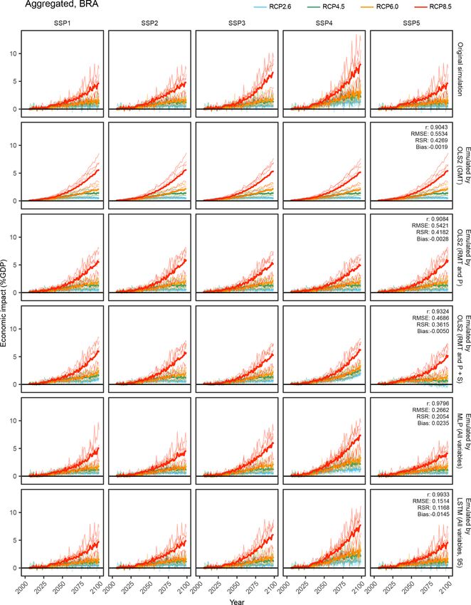
As illustrative examples, we explore simulated and em-
ulated results for chosen sectors in “Brazil” (Figs. 8, 9, and
10). The top row in each figure shows the time series of simu-
lated economic impacts for each scenario, and the remaining
rows show corresponding emulated economic impacts by dif-
ferent emulators. For aggregated economic impacts, general
tendencies could be reproduced even by simple emulators,
Figure 3. Performance of emulations in comparison 2. Correlation while complex emulators considering socioeconomic condi-
coefficients between simulation results and emulation results are tions could better represent subtle differences among SSPs
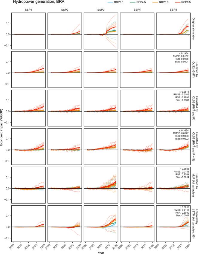
shown. (Fig. 8). For occupational-health cost sector and hydropower
generation sector impacts, obvious differences among SSPs
in the simulation results could not be reproduced by simple
were used (leftmost plots in each panel in Fig. 4), whereas emulators, but ANN-based complex emulators could repro-
MLP performed better when finer input variables were used duce the general tendencies (Figs. 9 and 10). For the hy-
(rightmost plots) in most cases. The relative importance of dropower generation sector, even the most complex emulator
variables differs depending on the modelled sectors. For ex- failed to reproduce some characteristics of the simulation re-
ample, for the agricultural productivity and undernourish- sults; that is, the emulator erroneously predicted discernible
ment sectors, the inclusion of socioeconomic variables in economic impacts under SSP1 and SSP4.
non-target regions contributed to the improvement in per- The performance of emulation can vary depending on how
formance. The performance for the fluvial flooding sector the training and test data are chosen. The results shown above
jumps when seasonal climate variables and climate variables are based on cross-validation with randomly selected scenar-
in non-target regions are used with MLPs. This is probably ios for training and testing. Figure 11 shows the compar-
due to the result of “leakage” (discussed later). ison of the performance between different cross-validation
Consideration of time-series input variables had positive procedures for the aggregated impacts as an example. Here,
effects for almost all sectors (Fig. 5), but it had greatest ef- the performance is shown by the RMSE normalized by the
fects in the hydropower generation sector (the median r im- pooled standard deviation (RSR), not by the correlation co-
proves from 0.48 to 0.78). This was mainly because LSTM efficient, because the standard deviation of each test data
could reproduce the pre-processing of bio/physical impact formulation, which affects the value of the correlation co-
simulations before inputting to the economic models. For ex- efficient, differs across the selected GCMs or RCPs. Sum-
ample, in the simulation of the hydropower generation sec- marized results for each sector and indices beyond RSR (r,
tor, calculated physical impacts (theoretical hydropower po- RMSE, and bias) are available in Tables S14 to S33 in the
tential) were averaged for every 20 years, and then tempo- Supplement. When the emulators were trained excluding the
ral linear interpolation was applied because this study fo- results of RCP8.5 (the highest emission pathway) and then
cused on long-term potential changes due to climate change tested by the results of RCP8.5 (RCP8.5 left condition), the
https://doi.org/10.5194/gmd-14-3121-2021 Geosci. Model Dev., 14, 3121–3140, 20213130 J. Takakura et al.: Reproducing complex simulations of economic impacts of climate change
Figure 4. Performance of emulations in comparison 3. Correlation coefficients between simulation results and emulation results are shown.
CA(1) denotes that climate variables for all regions (including non-target region) are used. CS(1) denotes that seasonal climate variables are
used. SA(1) denotes that socioeconomic variables for all regions (including non-target region) are used.
performance was apparently worse compared to the other 4 Discussion
conditions. Except for RCP8.5 left condition, the perfor-
mance was reasonably similar across conditions when sim- In this study, we developed various kinds of emulators and
pler models and input data were used. When complex mod- systematically evaluated their performance. We explored dif-
els and finer input variables were used, the performance was ferences in emulator performance among sectors and the re-
worse when cross-validated by GCM or cross-validated by lationship between model complexity and performance. The
RCP compared to the random cross-validation. aggregated economic impact was relatively easily emulated
The computational cost of the developed emulators was even by simple emulators with limited input variables. The
sufficiently small in the prediction phase, while training re- dominant contributors of aggregated impact were the heat-
quires some time for ANN-based emulators. Table 7 shows related excess mortality and occupational-health cost sectors
the computational cost for selected conditions. Even if the (Takakura et al., 2019) as also shown in Sect. S2 in the Sup-
most complex emulators are used, they require only 723 (679 plement, and the economic impacts of these two sectors were
to 1347) ms for the calculation of the economic impact for also relatively easily emulated. There were clear relation-
a century. From the viewpoint of computation time required ships between temperature rise and the simulated impacts in
for the prediction, both the OLS-based and ANN-based mod- these two sectors (Honda et al., 2014; Takakura et al., 2017),
els can meet the requirement of the emulators. However, it and almost all regions were impacted in the same direc-
should be noted that the time required to prepare the input tion. Moreover, where impacts were large, emulator perfor-
variables is not included in this assessment, and it depends mance tended to be better as shown in Fig. 7. Temperature-
on the situations. dependent impacts tend to be large and easy to emulate, while
precipitation-dependent impacts tend to be small and difficult
to emulate. Although it is not clear whether this correlation
reflects a causal relationship or is just a coincidence, these
Geosci. Model Dev., 14, 3121–3140, 2021 https://doi.org/10.5194/gmd-14-3121-2021J. Takakura et al.: Reproducing complex simulations of economic impacts of climate change 3131
Table 7. Computational cost of the developed emulators. Medians (minimum, maximum) of 17 regional, 9 sectoral, and aggregated impact
results are shown. OLS-based models and ANN-based models were implemented by the statsmodels library and Keras library in Python,
respectively. OLS2 (RMT + P + S): OLS2 with regional mean temperature precipitation and socioeconomic variables. MLP (RMT + P + S):
MLP with regional mean temperature precipitation and socioeconomic variables. MLP (All variables): MLP with all the input variables.
LSTM (All variables, 95): LSTM with all the input variables for 95 years.
Model Number of Number of Model object size Prediction time Training time
(input) input variables parameters (MB) (second/scenario) (second)
OLS2 1 3 1.470 0.002 0.010
(GMT) (1, 1) (3, 3) (1.470, 1.470) (0.002, 0.004) (0.008, 0.018)
OLS2 6 13 5.291 0.003 0.018
(RMT + P) (2, 10) (5, 21) (2.234, 8.348) (0.002, 0.015) (0.010, 0.029)
OLS2 9 19 7.583 0.004 0.022
(RMT + P + S) (5, 13) (11, 27) (4.527, 10.642) (0.003, 0.006) (0.014, 0.034)
MLP 9 1409 7.711 0.054 3.601
(RMT + P + S) (5, 13) (1281, 1537) (7.710, 7.711) (0.050, 0.133) (1.024, 13.349)
MLP 259 9409 7.711 0.134 6.552
(All variables) (259, 259) (9409, 9409) (7.711, 7.711) (0.129, 0.224) (1.375, 15.350)
LSTM 24 605 45 729 96.461 0.723 689.066
(All variables, 95) (24 605, 24 605) (45 729, 45 729) (96.454, 96.461) (0.679, 1.347) (153.160, 1761.409)
characteristics contributed to the higher performance of emu- are not considered explicitly (Kinoshita et al., 2018). We
lations of aggregated impacts particularly when simple func- suspect this is caused by the leakage because of the char-
tional forms were used. If we only focus on the aggregated acteristics of the simulation data used in this study. In the
economic impacts of climate change, a simple damage func- field of statistical machine learning, the word leakage means
tion which only leverages global mean temperature is worth that models have access to some information on the char-
using provided that we regard the original simulation results acteristics of the test dataset even if the test and training
as valid. On the other hand, some sectors’ and regions’ im- datasets are separated (Kaufman et al., 2011). In this study,
pacts were difficult to emulate by simple emulators, and con- we separated the dataset into training and test datasets de-
sideration of more input variables and more complex func- pending on the scenarios. When a certain scenario (for exam-
tional forms could improve the performance. Therefore, if we ple, SSP1-RCP2.6-HadGEM2-ES) is used in the test dataset,
focus on sectoral or regional issues (e.g. inequality among re- it is not included in the training dataset. By doing this, we
gions or sectors), conventional simple damage functions may can evaluate how the trained emulators will work when a
not be adequate tools and ANN-based or other complex tech- new unknown scenario is given. However, in the case of
niques may be necessary. fluvial flooding, the simulated impacts expressed by per-
For the agricultural productivity and undernourishment centage of GDP are very similar among SSPs (Takakura
sectors, the performance of the emulations was low unless et al., 2019). For example, the simulated impacts (percent-
socioeconomic conditions of non-target regions were incor- age of GDP) in SSP1-RCP2.6-HadGEM2-ES are almost
porated. Since comparative advantages (or disadvantages) identical to those in SSP2-RCP2.6-HadGEM2-ES, SSP3-
in the international food market and global food demands RCP2.6-HadGEM2-ES, SSP4-RCP2.6-HadGEM2-ES, and
play important roles in simulations of the impacts in these SSP5-RCP2.6-HadGEM2-ES, and some of these datasets are
sectors, it is reasonable that non-target regional information included in the training dataset. In such a situation, overfit-
contributed to improve the performance of the emulations. ting can result in apparently high performance in the cross-
Such beyond-the-border effects have not been considered in validation even if its actual ability for a new input dataset
previous studies using damage functions or emulators, but is low. Therefore, apparently high performance in the fluvial
our results shed light on the importance of this factor. It flood sector should be interpreted with caution.
is also noteworthy that these improvements were more dis- In the sectors of hydropower generation and thermal power
tinct when MLPs, which can represent complex interactions generation, even using the complex emulators with finer in-
among variables, were used as the emulators. put variables, the attained performance remained relatively
In terms of the results for the fluvial flooding sector, inclu- low. This implies that information required to reproduce the
sion of non-target regions’ quarterly climate variables with simulation results is missing from the input data. In the
MLP caused a drastic jump in the performance of the em- AIM/Hub model, there are SSP-dependent assumptions other
ulators. This is puzzling because in the simulation of the than population and GDP, particularly related to energy poli-
impacts of fluvial flooding, effects of international trading cies (Fujimori et al., 2017). These policies depend on the nar-
https://doi.org/10.5194/gmd-14-3121-2021 Geosci. Model Dev., 14, 3121–3140, 20213132 J. Takakura et al.: Reproducing complex simulations of economic impacts of climate change
Figure 5. Performance of emulations in comparison 4. Correlation Figure 6. Relationship between number of input variables and per-
coefficients between simulation results and emulation results are formance of emulators. Medians of 17 regional results are plotted
shown. MLP(1) denotes that MLPs are used as the emulators and as points. Fitted curves are produced for the frontiers (Pareto opti-
that only climatic and socioeconomic variables for the target year mal corresponding to each number of input variables) by beta re-
are used. LSTM(10) and LSTM(95) denote that LSTMs are used as gression. When time-series input data are used, the number of input
the emulators and that the climatic and socioeconomic variables for variables is multiplied by the length of the time series.
10 and 95 years are used, respectively.
To improve the performance of the economic impact em-
ulations, should we construct more complex emulators and
ratives of the SSP storylines, not just quantitative socioeco- consider more information? For example, in power gener-
nomic information such as population or GDP. In addition, ation sectors, model-specific assumptions regarding the en-
in the AIM/Hub model, adoption of power generation tech- ergy system could be used as additional input variables and
nology is decided by a discrete-choice model (Fujimori et this might improve the emulation performance. If a sufficient
al., 2014). Thus, the degree of reliance on a certain kind of number of simulation results are available, this strategy may
power generation can also be discrete or non-continuous de- work. An alternative approach is refraining from reproduc-
pending on the SSP-dependent assumptions in the AIM/Hub ing the complex behaviour of the energy system in the sim-
model. For example, a certain region does not rely on the hy- ulation model by an emulator and partly using the original
dropower generation at all in some situations, but once the simulation model. For example, in simulations of the im-
hydropower generation technology becomes economically pacts of hydropower generation and thermal power gener-
competitive compared to other power generation technolo- ation, bio/physical impacts (theoretical hydropower poten-
gies, hydropower generation plants will be installed in the tial and river flow) are simulated by a global hydrological
model. In the former situation, changes in the hydropower model, whose computational cost is high (around 15 to 20 h
generation capacity do not affect the economy at all, but they for one scenario), while the economic impacts are simulated
do in the latter situation. This difference cannot be predicted by an economic model, whose computational cost is rela-
by the emulators, since they cannot be represented only by tively low (around 1.5 h for one scenario) compared to that
climate conditions, GDP, and population. of the hydrological model. Therefore, if we can only emulate
Geosci. Model Dev., 14, 3121–3140, 2021 https://doi.org/10.5194/gmd-14-3121-2021J. Takakura et al.: Reproducing complex simulations of economic impacts of climate change 3133
of hidden layers, and the batch size for training in ANN –
can also be effective. In addition to optimizing or modifying
the models used in this study, other kind of models – such
as support vector regression, random forest regression, and
k-nearest neighbours regression – may also be effective. If
we adopt techniques like Gaussian process regression, un-
certainty of the predicted value can also be assessed. While
we did not investigate these techniques in this study, this rep-
resents an important direction for future research.
While there is substantial room for improvement, the em-
ulators developed in this study can be used as tools to ex-
plore various other future scenarios with limited computa-
tional and implementation cost. Technically, applying ANN-
based techniques to economic impact emulation is one of the
novelties of this study, and we have demonstrated that these
techniques can improve the performance of the emulations.
However, we do not claim researchers should always use
ANN-based (or similar statistically complex) techniques in
economic impact emulations. There is a non-negligible trade-
off between model complexity and performance. While com-
putational cost of emulation is small in the calculation (pre-
diction) phase as shown in Table 7, even by the most complex
emulator used in this study, the availability of input variables
Figure 7. Relationship between range of economic impacts (global) is context-specific. For example, the cost of preparing or gen-
and performance of emulators. Each point represents a sector, and erating sub-yearly regional climate variables should also be
the median of 17 regional results is plotted as the y axis value. Fitted considered. We disclose the source code for the OLS-based
curves are produced by beta regression. OLS2 uses only the global and ANN-based emulators developed herein. Sector-specific
mean temperature as the input variable, and LSTM uses all the pre- skills and knowledge are not necessarily needed to use this
pared input variables for 95 years.
code, and thus the implementation cost is much smaller than
that of the original simulation models, particularly if the
pre-trained models are used. Nevertheless, transplanting the
bio/physical impacts, the computational cost of economic ANN-based emulators to other modelling languages, if nec-
impact estimation can be reduced even if we use the origi- essary, is not always a trivial task, because of the required
nal simulation model for the economic part. Such model sep- software libraries. On the other hand, it is much easier to
arations will become important particularly if we focus, for transplant OLS-based emulators in any modelling language
example, on interactions among different sectors (Harrison because they only require arithmetic multiplication and addi-
et al., 2016). Another possibility is constructing SSP-specific tion.
emulators. In this study, since we aimed to explore new so- While sector-specific skills and knowledge are not always
cioeconomic pathways (e.g. intermediate pathway between necessary to use the developed emulators, users should be
SSP1 and SSP2), one common emulator was constructed for aware of the statistical context of the emulators and eval-
different socioeconomic pathways. On the other hand, if we uation results. Firstly, cross-validation is a powerful tool
fix the socioeconomic pathways to consider, it is possible to for evaluating the emulators’ performance without the influ-
incorporate SSP-specific assumptions into the emulators by ence of overfitting, and we can rely on the results of cross-
separating the models by SSPs. This option could be pursued validation to choose adequate models in most cases. How-
depending on the purpose of the studies. ever, leakage can pass the cross-validation test unlike simple
Even without introducing overly complex models or con- overfitting. While there is no perfect solution to detect the ex-
sidering excessively specific information, there are several istence of leakage, it can be effective to think about the actual
techniques which may improve the performance of emu- situation in which the developed emulators will be used. For
lation. For example, variable selection is a widely used example, if the emulators will be used to estimate economic
technique pursuant of developing parsimonious models and impacts under different RCPs or substantially different emis-
avoiding overfitting. We tested the simple step-wise variable sion pathways, which are not included in the training data,
selection based on Akaike’s information criterion, which can cross-validation by RCPs can be effective to estimate the ac-
easily be applied to an OLS-based technique, and the results tual performance of the emulators in that situation. Suspected
are shown in Sect. S3 in the Supplement. Optimization of leakage shown in Fig. 4 can be detected by this strategy
the hyperparameters – e.g. the number of units, the number (Sect. S4 in the Supplement). Secondly, regression models
https://doi.org/10.5194/gmd-14-3121-2021 Geosci. Model Dev., 14, 3121–3140, 2021You can also read