SHREC 2018 - Protein Shape Retrieval
←
→
Page content transcription
If your browser does not render page correctly, please read the page content below
SHREC 2018 – Protein Shape Retrieval
Florent Langenfeld1,* , Apostolos Axenopoulos2 , Anargyros Chatzitofis2 , Daniel Craciun1 , Petros Daras2 , Bowen Du3 , Andrea
  Giachetti4 , Yu-kun Lai5 , Haisheng Li3 , Yingbin Li3 , Majid Masoumi6 , Yuxu Peng7, 5 , Paul L. Rosin5 , Jeremy Sirugue1 , Li
   Sun3 , Spyridon Thermos2 , Matthew Toews6 , Yang Wei3 , Yujuan Wu3 , Yujia Zhai3 , Tianyu Zhao3 , Yanping Zheng3 , and
                                                      Matthieu Montes1,*,@
               1
                  Laboratoire GBA, EA4627, Conservatoire National des Arts-et-Métiers, 2 rue Conté, 75003 Paris, France
                          2 Information Technologies Institute, Centre for Research and Technology Hellas, Greece
 3 School of Computer Science and Information Engineering, Beijing Technology and Business University, No. 33 Fucheng Road, Haidian

                                                       District, Beijing 100048, P.R. China
                       4 Department of Computer Science, Università di Verona, Strada le Grazie 15, 37134 Verona
                        5 School of Computer Science and Informatics, Cardiff University, Cardiff, CF24 3AA, UK
                               6 École de Téchnologie Supérieure, University of Québec, Montréal, QC, Canada
    7 School of Computer and Communication Engineering, Changsha University of Science and Technology, Changsha, 410114, Hunan

                                                                  Province, China
                                                                 * Track organizers
                                      @ Corresponding author: Matthieu Montes, matthieu.montes@cnam.fr

                                                      March 22, 2018

                                                             Abstract
         Proteins are macromolecules central to biological processes that display a dynamic and complex surface.
     They display multiple conformations differing by local (residue side-chain) or global (loop or domain) structural
     changes which can impact drastically their global and local shape. Since the structure of proteins is linked to
     their function and the disruption of their interactions can lead to a disease state, it is of major importance to
     characterize their shape. In the present work, we report the performance in enrichment of six shape-retrieval
     methods (3D-FusionNet, GSGW, HAPT, DEM, SIWKS and WKS) on a 2 267 protein structures dataset generated
     for this protein shape retrieval track of SHREC’18.

1     Introduction                                                   tion of their interactions can lead to a disease state, it
                                                                     is of major importance to characterize their shape as it
                                                                     will allow the identification of potential binders such as
The goals of structural biology include developing a                 other proteins, drugs or nucleic acids.
comprehensive understanding of the molecular shapes
and forms embraced by biological macromolecules and                     Since most shape-retrieval methods are not dedicated
extending this knowledge to understand how differ-                   to protein shape comparison, we generated two version
ent molecular architectures are used to perform most                 of the dataset for the participants: original Protein Data
biological processes. Among these macromolecules,                    Bank files [4] (which describe the atomic coordinates
proteins are critical effectors involved in most pro-                of a protein) and the mesh of the Solvent Excluded Sur-
cesses and display a dynamic and complex surface.                    face (SES) of the protein [8] in OFF (Object File For-
They can be composed of hundreds of thousands atoms                  mat) format. All data was extracted from high resolu-
and display multiple conformations differing by local                tion structures to stay as close as possible to a real-life
(residue side-chain) or global (loop or domain) struc-               case study.
tural changes at the atomic scale which can drastically                The dataset included identical, structurally similar
impact their global and local shape. Since the structure             and structurally different proteins. The dataset is com-
of proteins is linked to their function and the disrup-              posed of 2 267 unique structures distributed into 107

                                                                 1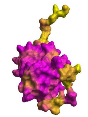
classes. The participants were asked to compare the 2                 2. The dataset was limited to protein domains with no
267 structures for their surface dissimilarity. The num-                 more than 200 residues.
ber of classes was not provided to best match a real-
world blind study. Six groups using six different meth-               3. “Artifacts”, “Low resolution protein structures”
ods returned their results that are reported in the present              and “automated matches” branches of the SCOPe
work.                                                                    tree were not retained.

                                                                      4. Structures in complex with small molecules or dis-
                                                                         playing modified residues were not retained.
2      Data Set
                                                                      5. Highly homologous domains from 7 PDB struc-
To reflect the ability of the methods to retrieve the                    tures, namely 1ed7, 1f40, 1j6y, 1qnz, 2gri, 2kn5
different surfaces representing the same protein do-                     and 2rr9 [15, 27, 16, 28, 25, 11, 24] were added.
main, we relied on the reference database of pro-
tein structures, the Protein Data Bank (PDB) [4], and                 6. We separated individual domains of multi-domain
on the Structural Classification of Proteins - extended                  structures, individual chains from multi-chain
(SCOPe) database [10, 7] to build relations between dis-                 structures, and individual conformers.
tinct PDB entries.
   The Protein Data Bank is the world-wide reposi-                   In total, from the 79 PDB structures describing 88 do-
tory for experimental biological macro-molecules. In              mains, we retained 2 267 individual structures separated
February 2018, it comprised 137 917 entries, describ-             in 107 classes. 18 out of the 107 classes were populated
ing 42 193 distinct protein sequences. Version 2.06               by only one conformer while the biggest class displayed
of the SCOPe database contained 77 439 PDB entries                110 conformers. The average class size was 21.18.
distributed over 244 326 domains, the lowest-level of                All PDB files generated were further cleaned and pre-
the SCOPe classification tree. Highest levels (class              pared using the pdb4amber routine of AmberTools [6]:
and fold) are discriminated according to structure/shape          water molecules were removed while missing atoms, if
while lowest levels (superfamily, family, protein and             any, were added. The resulting structures were submit-
species) are built on evolutionary concerns. We de-               ted to participants in PDB format.
fined the dataset classes as domains with the same par-
                                                                     The EDTSurf program [30] was used to generate the
ent at the species level of the SCOPe database, ensur-
                                                                  Solvent Excluded Surface [8] of each structure. Stan-
ing that domains from the same class were identical.
                                                                  dard parameters were used. The inner surface was not
Thus, intra-class relations were established if and only
                                                                  computed. An in-house script was used to convert PLY
if two SCOPe domains displayed the same species par-
                                                                  files to OFF files. These 2 267 OFF files were submitted
ent, while all other relations were considered as extra-
                                                                  to participants.
class. Below, is an extensive description of our protocol
to build up the dataset.
   First, the SCOPe database tree was built. Conse-
quently, the same domains found in different PDB en-
                                                                  3      Evaluation
tries were gathered into the same leaves of the tree, al-
                                                                  Normalized Discounted Cumulative Gain
lowing the selection of PDB entries while keeping the
intra-class information. Since 244 326 domains were               The Discounted Cumulative Gain (DCG) is a weighted
implemented in the SCOPe database, we applied the                 statistics assuming that correct results associated with a
following filters to restrict the size of the dataset to a        higher rank should imply a gain in the performance rat-
manageable order of magnitude for the participants.               ing as users are more likely to consider these results.
                                                                  For a list R of correct results, a list G is generated,
    1. To reflect the experimentally observed variability         where Gi is 1 if element Ri is in the correct class (the
       of protein conformations, we selected only Nu-             ground truth class associated with element i GTi ), or 0
       clear Magnetic Resonance (NMR) structures [29]             otherwise.
       that usually contain several conformations of the             The Discounted Cumulative Gain is then computed
       same protein.                                              using the following:

                                                              2
4 Participants & Methods
G1 , if i = 1 4.1 3D convolutional framework for pro-
DCGi = Gi
DCGi−1 + log2 (i) , otherwise
tein shape retrieval (3D-FusionNet),
by S. Thermos, A. Chatzitofis, A.
This value is then divided by the maximal value pos-
sible (i.e. the value obtained by the ground truth) as
Axenopoulos and P. Daras
follows: Problem Definition
DCGk
DCG = P|C| The idea behind the proposed framework is to combine
1 + j=2 log12 (j)
state-of-the-art hand-crafted descriptors that effectively
represent the 3D molecular shape with the features ex-
where k is the number of objects in the dataset and C
tracted using a deep Neural Network (NN). The NN has
the size of the classes. This value is a good summary for
been trained on a different dataset of flexible molecules,
a comparative evaluation of the performance of differ-
the MOLMOVDB [9]. The input 3D model is the Sol-
ent methods performance. A normalized value nDCG
vent Excluded Surface (SES) of a protein molecule,
of the DCG is therefore computed over all methods,
which has been created from the molecule’s tertiary
and compared to the average value aveDCG:
structure (PDB format) using the EDTSurf software.
This software produces a high-resolution watertight tri-
DCGalgo
nDCGalgo = −1 angulated mesh. The triangulated mesh is simplified
aveDCG and used as input to the algorithm that extracts the hand-
where a negative value indicated that the perfor- crafted features, while for the deep NN architecture a
mance of the method is under the average while a posi- 32 × 32 × 32 voxel model is created.
tive value indicated that the performance of the method
is over the average. The norm of the value indicates the A Shape Descriptor Based on Diffusion Distances
gap to the average performance.
Extraction of hand-crafted features is based on the com-
bined DDMR shape descriptor, which has been intro-
Nearest Neighbor, First-tier and Second-tier duced in [3], and it is invariant to protein conforma-
tions. At a pre-processing stage, the high-resolution
These parameters check the ratio of models that belong
mesh is simplified resulting in a set of NS uniformly
to the same class as the query. For Nearest Neighbor,
sampled points that provide a coarse representation of
the first match only is considered, while the |C| − 1 and
the 3D molecule. At the descriptor extraction step, the
2 ∗ (|C| − 1) first matches are considered for First-tier
Modal Representation of the Diffusion-Distance Matrix
and Second-tier parameters.
(DDMR descriptor) is extracted. DDMR is a global
shape descriptor, which is produced by applying Sin-
Precision-Recall plot and E-measure gular Value Decomposition on the Diffusion Distance
Matrix of all NS oriented points, keeping the first n sin-
Precision P represents the ratio of models from class C gular values (n = 40 in our experiments). The diffusion
retrieved within all objects attributed to class C, while distance between two points on a surface is considered
Recall R represents the ratio of models from class C as an average length of paths connecting the points in a
retrieved compared to |C|. sense of inner distances and it is able to capture topo-
The E − measure is a composite parameter of both logical changes in molecular shapes [18].
Precision and Recall:
2 Volumetric Binary Grid
E − measure = 1 − 1 1
P + R Based on the approach of Nooruddin and Turk [23],
we rasterize the protein 3D model to a binary voxel
All analyses were done using the Princeton Shape grid. The 3D models of the proteins are watertight, thus
Benchmark utilities [26]. the parity count method is applied for binary voxeliza-
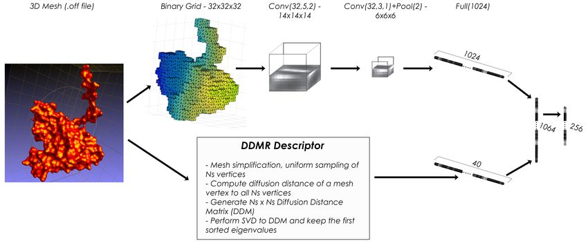
3Figure 1: The proposed fusion architecture that consists of a VoxNet [22] CNN (top information stream), fol-
lowed by a MLP model (right-most). The latter fuses the VoxNet-extracted and the hand-crafted features (bottom
information stream), respectively.
tion. To this end, a voxel v is classified by counting For the protein shape retrieval, a transfer learning ap-
the number of times that a line crossing the center of proach is adopted. At first, the fusion architecture is
the voxel intersects polygons of the 3D model surface. trained on the MOLMOVDB dataset [9] which consists
Ray-casting the 3D model with parallel rays, all of the of over 200 classes of proteins. Subsequently, the Soft-
voxels along the ray are classified. For an odd num- max layer is dropped and the architecture is used for
ber of intersections, voxel v is considered interior to feature extraction. For each previously unseen input,
the model, while for an even number, outside. For a a feature vector is extracted. After the completion of
N × N × N voxel grid resolution, where N = 32, we the feature extraction, the Euclidean distance metric is
cast N ×N = 1024 rays, with each ray passing through used to measure the distance between the evaluated in-
N-voxel centers. put models. Small distance values indicate that the cor-
responding feature vectors represent the same protein
class.
Fusion Architecture
The proposed architecture, depicted in Fig. 1, con-
sists of a convolutional neural network (CNN), utilized
for 3D shape representation learning, followed by a
4.2 Global Spectral Graph Wavelet
Multi-Layer Perceptron (MLP), which fuses the CNN- framework (GSGW), by M. Masoumi
extracted features with the hand-crafted descriptors pre- and M. Toews
sented in Section “A Shape Descriptor Based on Dif-
fusion Distances”. In detail, the VoxNet CNN [22] is Our global spectral graph wavelet (GSGW) frame-
used, which consists of 2 volumetric convolutional lay- work [21] is based on the eigensystem of the Laplace-
ers, 1 max pooling layer and 3 fully connected layers, Beltrami operator that are invariant to isometric trans-
and efficiently encodes the spatial structures such as formations. GSGW is a multi-resolution descriptor that
planes and corners at different scales and orientations. incorporates the vertex area into the definition of spec-
The VoxNet processes the voxel inputs and the features tral graph wavelet [20, 19] in a bid to capture more
after its last fully connected layer are concatenated with geometric information and, hence, further improve its
the corresponding hand-crafted ones. The latter are pro- discriminative ability. GSGW also provides a general
cessed by the MLP followed by a Softmax layer used and flexible interpretation for the analysis and design of
for classification. spectral descriptors. For a vertex j of a triangle mesh,
4spectral graph wavelet is defined as [20]: the proposed approach, we set the resolution parameter
to R = 30 (i.e. the spectral graph wavelet signature ma-
sL (j) = {Wδj (tk , j) | k = 1, . . . , L} ∪ {Sδj (j)}, (1) trix is of size 495 × m, where m is the number of mesh
vertices).
where Wδj (tk , j) and Sδj (j) are the spectral graph
wavelet and scaling function coefficients at resolution
level L, respectively. We then represent a shape M by a 4.3 Histograms of Area Projection Trans-
p-dimensional vector form (HAPT), by A. Giachetti
m
X In our runs, we characterized the protein shapes with the
x = Sa = ai si , (2) Histograms of Area Projection Transform (HAPT) [12].
i=1 The method, usually well suited for nonrigid shape re-
trieval, is based on a spatial map (Multiscale Area Pro-
where S = (s1 , . . . , sm ) is a p×m matrix of local spec- jection Transform) that encodes the likelihood of the
tral graph wavelet signatures and a = (a1 , . . . , am )| is 3D points inside the shape of being centres of spheri-
an m-dimensional vector of mesh vertex areas (i.e. each cal symmetry. This map is obtained by computing, for
element ai is the area of the Voronoi cell at mesh vertex each radius of interest, the value:
i).
We refer to the p-dimensional vector x as the global AP T (~x, S, R, σ) = Area(TR−1 (kσ (~x) ⊂ TR (S, ~n)))
spectral graph wavelet (GSGW) descriptor of the pro- (3)
tein surface. The GSGW descriptor enjoys a number where S is the surface of the object, TR (S, ~n) is the
of desirable properties including simplicity, compact- parallel surface of S shifted along the normal vector ~n
ness, invariance to isometric deformations, and compu- (only in the inner direction) and kσ (~x) is a sphere of ra-
tational feasibility. Moreover, GSGW combines the ad- dius σ centred in the generic 3D point ~x where the map
vantages of both band-pass and low-pass filters. is computed. Values at different radii are normalized in
Our proposed protein shape retrieval algorithm con- order to have a scale-invariant behaviour, creating the
sists of four main steps. In the first step, we represent Multiscale APT (MAPT):
each protein in the dataset by a spectral graph wavelet M AP T (~x, R, S) = α(R) AP T (~x, S, R, σ(R)) (4)
signature matrix, which is a feature matrix consisting of
local descriptors. More specifically, let D be a dataset where α(R) = 1/4πR2 and σ(R) = c · R (0 < c <
of n proteins modeled by triangle meshes M1 , . . . , Mn . 1).
We represent each surface Mi in the dataset D by A discretized MAPT is easily computed, for selected
a p × m spectral graph wavelet signature matrix Si , values of R, on a voxelized grid including the surface
whose columns are p-dimensional local signatures and mesh, with the procedure described in [12]. The map
m is the number of mesh vertices. In the second step, is computed in a grid of voxels with side s on a set of
we compute the p-dimensional global spectral graph corresponding sampled radius values R1 , ..., Rn .
wavelet descriptor xi = Si ai of each protein Mi , for For the proposed task, discrete MAPT maps were
i = 1, . . . , n. Subsequently, the feature vectors xi of all quantized in 8 bins and histograms computed at the
n shapes in the dataset are arranged into a n×p data ma- selected scales (radii) were concatenated creating an
trix X = (x1 , . . . , xn )| . In the third step, we calculate unique descriptor. Voxel side and sampled radii were
volume v and surface area a of each 3D model Mi and fixed set for each run and chosen to represent the ap-
then aggregate them to X to provide further discrimina- proximate radii of the spherical symmetries visible in
tion power for GSGW. Finally, we compare a query x the models. We tested two different options, in the first
to all data points in X using `1 -distance to find the most (runs 1 and 2) we put s = 1 and we computed the
relevant shapes to the query. The lower the value of this MAPT histograms for 8 increasing radii starting from
distance is, the more similar the shapes are. R1 = 1 iteratively adding a fixed step of 1 for the re-
The experiments were conducted on a laptop with an maining values {R2 , . . . , R8 }. For the second (runs 3
Intel Core i7 processor running at 2.00 GHz and 16 GB and 4), we put s = 0.5 and we computed the MAPT his-
RAM; all the algorithms were implemented in MAT- tograms for 8 increasing radii starting from R1 = 0.5
LAB. In our setup, a total of 31 eigenvalues and asso- iteratively adding a fixed step of 0.5 for the remaining
ciated eigenfunctions of the LBO were computed. For values {R2 , . . . , R8 }.
5The procedure for model comparison then simply belonging to the 2D grids. The MAD distance is com-
consists in concatenating the MAPT histograms com- puted over the minimum number of points belonging to
puted at the different scales and measuring distances be- the overlapping area computed between the query and
tween shapes by evaluating the Euclidean distance (runs the target meshes.
1 and 3) and the Jeffrey divergence (runs 2 and 4) of the
corresponding concatenated vectors. Runtime Evaluation
The estimation of the descriptors took on average 1.4
sec per model with the first discretization option, 2.4 The MS-DEM descriptor computation for file 1 (shown
with the second on a laptop with an Intel® Core™ i7- in Figure 2) is performed in 8 seconds on a 64b Linux
4720HQ CPU running Ubuntu Linux 16.04. The de- machine, equipped with 32Gb of RAM memory and an
scriptor comparison time was negligible. Intel Xeon @ 3.40 GHz. The mean runtime for MS-
DEM Comparison is 7.1396· 10−4 sec corresponding to
a mean number of compared points in the overlapping
4.4 Protein Shape Retrieval driven by area of 7.9795· 104 points.
Digital Elevation Models (DEM), by
D. Craciun, J. Sirugue and M. Montes Scale-invariant wave kernel signature (SI-
The molecular shape similarity system is composed of WKS), by Y. Wu, Y. Zheng, L.i Sun, Y. Li,
two main stages: the first stage is performed for each T. Zhao, B. Du, Y. Zhai, Y. Wei and H. Li
shape and consists in the global shape representation as In this track, we propose a new feature for 3D
a Digital Elevation Model (DEM), encoded over a 2D shape retrieval called scale-invariant wave kernel sig-
grid; te second stage corresponds to the shape compar- nature(SIWKS). The process can be described as fol-
ison phase supplied via global distance measures com- lows. Firstly, the WKS represents the average proba-
puted over the DEMs. bility of measuring a quantum mechanical particle at a
specific location. By letting vary the energy of the par-
Representing Macromolecular Shapes as Digital El- ticle, the WKS encodes and separates information from
evation Models various different Laplace eigenfrequencies. Based on
the Schrödinger equation each point on an object’s sur-
The shape representation algorithm applies the EDT- face is associated with a Wave Kernel Signature. Then,
Surf [30] technique to generate the macromolecular sur- we found that WKS is the sensitivity to scale transfor-
face (MS) from the input data. The descriptor compu- mation. We bring the spirit of eigenvalue normalization
tation stage starts by applying the mesh flattening pro- based methods to construct a scale invariant wave ker-
cedure used to map the mesh onto the unit sphere using nel signature. Finally, the scale factor in WKS is re-
the Laplace-Beltrami operator, resulting in an isome- moved.
try invariant shape representation [1, 13]. In the sec-
ond step, the unit sphere is projected onto a 2D spheri- (
cal panoramic grid and the elevation values of the input W KS(x, · ) : R → R
W KS −(ei −logλi )2
mesh are assigned to each 2D location of the panoramic W KS(x, e) = Ce i φ2i (x)e
P
2σ 2
grid. This results in a global descriptor which en- (5)
codes elevation values, while providing topology and
fast comparison over a 2D grid space. The final output (
is the Digital Elevation Model associated to the macro- SIW KS(x, · ) : R → R
SIW KS φ2i (x) −(ei −logλi)
2
molecular surface, noted MS-DEM. Figure 2 illustrates
P
SIW KS(x, e) = Ce i λi e
2σ 2
the results obtained for the file 1 belonging to the pro- (6)
tein pool of the SHREC 2018 track. where
!−1
X −(ei −logλi )2
Global Comparison of MS-DEMs Ce = e 2σ 2
i
The present research work evaluates the Mean Absolute
Differences (MAD) which is measured over the points in equations (5) and (6).
6Figure 2: Results obtained for the global descriptor computation stage for file 1: (a) PDB input: 96 642 points,
184 080 triangles, (b) macromolecular mesh generated by the EDTSurf method [30]: 95 505 points, 191 022
triangles, (c) spherical mapping output: 95 505 points, 191 022 triangles; (d) MS-DEM descriptor output: 95 505
points.
4.5 Wave Kernel Signature (WKS), by Y. ues.
Peng, Y. Lai and P. L. Rosin WKS is computed from the eigenvalues
and the eigenvectors. We use the code from
In recent years, significant attention has been devoted https://github.com/ChunyuanLI/
to descriptors obtained from the spectral decomposi- spectral_descriptors [17]. We set the
tion of the Laplace-Beltrami operator associated with number of features to 100 and the variance is 100 × 5.
the shape. Notable examples in this family are the The vocabulary of the WKS feature is created.
Heat Kernel Signature (HKS) and the recently intro- The size of vocabulary is chosen as 1 000 accord-
duced Wave Kernel Signature (WKS) [2]; the latter is ing to our experiments on the subset of the FSSP
described in the previous section. They are compu- database [3, 14]. The size of the feature vec-
tationally efficient, isometry-invariant by construction, tor at each vertex on the mesh is 50 and normal-
and can gracefully cope with a variety of transforma- ized. Then we randomly select 10% of the mesh
tions. points and apply Ovsjanikov’s improved k-means algo-
rithm (http://www.lix.polytechnique.fr/
˜maks/code/shapegoogle_code.zip) [5] to
generate the vocabulary.
We compute the Bag of Features (BoFs) for each pro-
tein using hard Vector Quantization. The feature is a
1000 × 1 vector and normalized.
The distance between the BoFs of any two proteins is
computed using the L1 distance kX − Y k1 . For a given
query shape, the shapes from the dataset are retrieved
based on this distance.
Figure 3: Protein mesh coloured according to the WKS 5 Results
feature
Each team submitted one to four 2267 × 2267 dissim-
The eigenvalues and the eigenvectors are obtained ilarity matrices resulting in 9 methods to evaluate. The
from protein mesh files in our experiment. We use following section summarizes the performance in re-
the MeshLP package to compute the eigenvalues and trieval for each method, and insights are given regarding
the eigenvectors of the Laplace operator on the mesh. the number of conformers in each class. Three types
The time axis is sampled logarithmically. The code is of classes were defined: small classes contained less
modified from https://github.com/areslp/ than 20 conformers, medium classes contained 20 to 40
matlab/tree/master/HKS/ and uses default val- conformers, and large classes contained at least 41 con-
7formers. classes were significantly lower for all methods com-
pared to other classes, except for HAPT methods 2-
4 whose First-tier statistics were better for the small
5.1 Overall results classes than for the other classes. Each method dis-
The results summarized in Table 1 were computed played distinct Nearest Neighbor, First-tier and Second-
for each dissimilarity matrix (3D-FusionNet, HAPT1, tier performances depending on the type of class (small,
HAPT2, HAPT3, HAPT4, SIWKS, DEM, WKS and medium or large). The mean Nearest Neighbor value
GSGW) over all classes and over each type of class for small classes was 0.278 (the highest value was 0.418
(small, medium or large). Overall, the Histograms of for HAPT4) and First-tier mean value was 0.392 (only
Area Projection Transform (HAPT) method displayed HAPT2-4 runs displayed First-tier values above 0.5).
the best results, especially for the run 4 which showed On the contrary, for medium and large classes, Nearest
the best results for all statistics. Wave Kernel Signature Neighbor parameters were significantly increased com-
based Shape Descriptor (WKS) and 3D convolutional pared to small classes, whereas First-tier and Second-
framework for protein shape retrieval (3D-FusionNet) tier statistics decreased. This behavior is particularly
displayed similar overall results, close to the HAPT marked for large classes where Nearest-Neighbor dis-
runs. Digital Elevation Models (DEM) and Global played a mean value of 0.706 while First-tier mean
Spectral Graph Wavelet framework (GSGW) methods value is 0.254, which is lower than the First-tier mean
followed in performance, and the Scale-invariant Wave value for small classes (0.392).
Kernel Signature (SIWKS). Similar trends are observed Last, depending on the number of conformers in
with the Precision-Recall curves (Figure 4). each class, the respective performances of the meth-
ods varied. As an example, the normalized Dis-
1.0
Method counted Cumulative gain (nDCG) of HAPT4 for small
0.9 3D-FusionNet
0.8
DEM
GSGW
classes was 24.89% while it was 17.24% and 6.91%
0.7
HAPT1
HAPT2
for medium and small classes respectively. Conversely,
HAPT3
0.6 HAPT4 the DEM method display a normalized Discounted Cu-
Recall
SIWKS
0.5
WKS mulative Gain of -31.51%, -15.93% and -8.20% for
0.4
0.3
small, medium and large classes respectively. Thus, the
0.2 data set composition could influence the choice of the
0.1
method: for large classes, 3D-FusionNet, HAPT4 and
0.0
0.0 0.2 0.4 0.6 0.8 1.0 WKS displayed similar performances, while for small
Precision
classes, HAPT4 outperformed the other methods.
A comparable analysis was performed based on the
Figure 4: Precision-Recall curves. Each curve corre-
size of the proteins (number of atoms in the PDB files)
sponds to a dissimilarity matrix provided by a partici-
and the size of the meshes (number of vertices in the
pant to the track
OFF files). No clear pattern was extracted from this
analysis, except for the Nearest Neighbor statistics that
is inversely correlated to the size of the system (either
5.2 The number of conformers impacts expressed as the number of atoms or the number of ver-
the methods’ performance tices). The smaller the system is, the better the methods
performed in terms of Nearest Neighbor retrieval.
We computed the Nearest Neighbor, First-tier, Second-
tier, E-measure, Discounted Cumulative Gain statistics
and normalized Discounted Cumulative Gain statistics 6 Discussion
over the whole dataset for all methods. The values of
all statistics for all methods were then computed for the Proteins are linear chains of amino-acids who fold into
small, medium and large classes (Table 1). a broad variety of 3D shapes. They are intrinsically dy-
As expected, all methods performed better on large namic objects whose motions, hence their surface and
classes (more than 40 conformers in the class) than their shape, are directly related to their activity. Many
on medium classes (20-40 conformers) or small classes parameters influence the protein dynamics and/or fold-
(less than 20 conformers). The performances for small ing: the amino-acids composition of the protein or the
8Table 1: Results summary by method and by size of the classes. Normalized DCG for small, medium and
large classes are computed with respect to the average DCG of small, medium and large classes, respectively.
NN = Nearest Neighbor, Tier1 = First-tier, Tier2 = Second-Tier, DCG = Discounted Cumulative Gain, nDCG =
normalized Discounted Cumulative Gain.
Method Class NN Tier1 Tier2 E-measure DCG nDCG (%)
3D-FusionNet All 0.689 0.404 0.459 0.366 0.681 3.92
Small 0.297 0.394 0.255 0.253 0.496 -0.94
Medium 0.672 0.468 0.524 0.397 0.693 3.52
Large 0.822 0.287 0.323 0.319 0.697 6.08
HAPT1 All 0.713 0.413 0.534 0.409 0.719 9.72
Small 0.390 0.456 0.306 0.288 0.573 14.53
Medium 0.716 0.503 0.630 0.462 0.748 11.71
Large 0.782 0.280 0.310 0.301 0.676 2.82
HAPT2 All 0.703 0.439 0.541 0.415 0.72 9.87
Small 0.357 0.522 0.335 0.314 0.592 18.34
Medium 0.693 0.509 0.632 0.466 0.746 11.44
Large 0.799 0.283 0.315 0.304 0.678 3.15
HAPT3 All 0.712 0.459 0.56 0.433 0.734 12.00
Small 0.276 0.549 0.339 0.330 0.590 17.92
Medium 0.714 0.542 0.663 0.490 0.766 14.38
Large 0.813 0.278 0.308 0.311 0.685 4.21
HAPT4 All 0.77 0.493 0.584 0.462 0.755 15.21
Small 0.418 0.613 0.358 0.373 0.625 24.89
Medium 0.768 0.578 0.688 0.515 0.785 17.24
Large 0.854 0.300 0.315 0.338 0.702 6.91
SIWKS All 0.199 0.109 0.189 0.114 0.452 -31.03
Small 0.112 0.111 0.067 0.078 0.333 -33.40
Medium 0.183 0.102 0.190 0.118 0.432 -35.56
Large 0.257 0.142 0.207 0.123 0.534 -18.73
DEM All 0.421 0.238 0.319 0.231 0.555 -15.31
Small 0.088 0.158 0.079 0.113 0.343 -31.51
Medium 0.428 0.277 0.370 0.262 0.563 -15.93
Large 0.551 0.196 0.250 0.205 0.603 -8.20
WKS All 0.717 0.41 0.49 0.377 0.701 6.97
Small 0.288 0.417 0.281 0.264 0.522 4.24
Medium 0.718 0.473 0.561 0.416 0.720 7.53
Large 0.805 0.294 0.347 0.313 0.702 6.78
GSGW All 0.514 0.261 0.35 0.247 0.581 -11.34
Small 0.272 0.306 0.197 0.166 0.430 -14.08
Medium 0.476 0.281 0.373 0.264 0.574 -14.34
Large 0.674 0.230 0.302 0.223 0.637 -3.03
presence of a given substance (ion, ligand, nucleic acid The ground truth was designed with this aim, and there-
or protein) drive the protein conformation to another fore relied on the protein sequence only. Other con-
and therefore may modulate its function. To date, high- siderations (active vs inactive states of proteins for ex-
resolution experiments have been able to determine the ample) may constitute a new viewpoint to propose new
structure of more than 130 000 proteins [4]. datasets for a future track.
Here, we designed a dataset to evaluate the ability of We only included proteins of small to medium size
shape retrieval methods to identify protein shape varia- (less than 200 residues) to limit the size of the resulting
tions, and more specifically to distinguish between vari- high resolution meshes. Besides, we only selected 79
ations due to the protein dynamics and variations due NMR structures which are generally structures of small
to the protein sequence (the amino-acids composition). proteins. This is far from representing the protein size
9diversity contained in the Protein Data Bank. Introduc- [4] H. M. Berman, J. Westbrook, Z. Feng,
ing X-ray crystallographic structures or more recently G. Gilliland, T. N. Bhat, H. Weissig, I. N.
deposited high resolution Cryo Electronic microscopy Shindyalov, and P. E. Bourne. The Protein Data
structures would be more representative of the diversity Bank. Nucleic Acids Research, 28(1):235–242,
of the systems available in the PDB. 2000.
As presented in the results section, we observed var-
ious performances depending on the size of the classes: [5] A. M. Bronstein, M. M. Bronstein, L. J. Guibas,
all methods displayed a better performance on lesser and M. Ovsjanikov. Shape google: Geomet-
populated classes within the First-tier while they dis- ric words and expressions for invariant shape re-
played a better Nearest-Neighbor performance on more trieval. ACM Trans. Graph., 30(1):1:1–1:20, Feb.
populated classes. All methods did not perform uni- 2011.
formly over all the classes in terms of enrichment. [6] D. Case, D. Cerutti, T. Cheatham, III, T. Dar-
Finally, due to the size of protein structure databases den, R. Duke, T. Giese, H. Gohlke, A. Goetz,
(>130 000 structures in the PDB in 2018, roughly 10 D. Greene, N. Homeyer, S. Izadi, A. Kovalenko,
000 to 15 000 new structures each year), it would be T. Lee, S. LeGrand, P. Li, C. Lin, J. Liu,
of importance to consider the computational time in the T. Luchko, R. Luo, D. Mermelstein, K. Merz,
methods performances as well, with the aim to screen in G. Monard, H. Nguyen, I. Omelyan, A. Onufriev,
a near future a datasets of hundreds of thousands protein F. Pan, R. Qi, D. Roe, A. Roitberg, C. Sagui,
structures. C. Simmerling, W. Botello-Smith, J. Swails,
R. Walker, J. Wang, R. Wolf, X. Wu, L. Xiao,
D. York, and P. Kollman. Amber 2017. University
Acknowledgements of California, San Francisco, 2017.
D. Craciun, J. Sirugue and M. Montes research [7] J.-M. Chandonia, N. K. Fox, and S. E. Bren-
work is supported by the ERC ViDOCK Grant no. ner. SCOPe: Manual curation and artifact removal
#640283 from the European Research Council Exec- in the Structural Classification Of Proteins – ex-
utive Agency. Y. Peng, Y. Lai and P. L. Rosin re- tended database. Journal of Molecular Biology,
search work is supported by China Scholarship Coun- 429(3):348 – 355, 2017. Computation Resources
cil(CSC,20170080005). for Molecular Biology.
[8] M. L. Connolly. Analytical molecular surface
calculation. Journal of Applied Crystallography,
References 16(5):548–558, Oct 1983.
[1] S. Angenent, S. Haker, A. Tannenbaum, and [9] N. Echols, D. Milburn, and M. Gerstein. Mol-
R. Kikinis. On the Laplace-Beltrami operator and MovDB: analysis and visualization of conforma-
brain surface flattening. IEEE Transactions on tional change and structural flexibility. Nucleic
Medical Imaging, 18(8):700–711, Aug 1999. Acids Research, 31(1):478–482, 2003.
[2] M. Aubry, U. Schlickewei, and D. Cremers. The [10] N. K. Fox, S. E. Brenner, and J.-M. Chando-
wave kernel signature: A quantum mechanical ap- nia. SCOPe: Structural Classification Of Pro-
proach to shape analysis. In 2011 IEEE Interna- teins—extended, integrating SCOP and ASTRAL
tional Conference on Computer Vision Workshops data and classification of new structures. Nucleic
(ICCV Workshops), pages 1626–1633, Nov 2011. Acids Research, 42(D1):D304–D309, 2014.
[3] A. Axenopoulos, D. Rafailidis, G. Papadopoulos, [11] G. D. Friedland, N.-A. Lakomek, C. Griesinger,
E. N. Houstis, and P. Daras. Similarity search J. Meiler, and T. Kortemme. A correspondence
of flexible 3D molecules combining local and between solution-state dynamics of an individual
global shape descriptors. IEEE/ACM Transac- protein and the sequence and conformational di-
tions on Computational Biology and Bioinformat- versity of its family. PLOS Computational Biol-
ics, 13(5):954–970, September 2016. ogy, 5(5):1–16, 05 2009.
10[12] A. Giachetti and C. Lovato. Radial sym- recognition. In 2015 IEEE/RSJ International Con-
metry detection and shape characterization ference on Intelligent Robots and Systems (IROS),
with the multiscale area projection transform. pages 922–928, Sept 2015.
Comp.Graph.Forum, 31(5):1669–1678, 2012.
[23] F. S. Nooruddin and G. Turk. Simplification and
[13] C. Gotsman, X. Gu, and A. Sheffer. Fundamen- repair of polygonal models using volumetric tech-
tals of spherical parameterization for 3D meshes. niques. IEEE Transactions on Visualization and
ACM Trans. Graph., 22(3):358–363, July 2003. Computer Graphics, 9(2):191–205, April 2003.
[14] L. Holm and C. Sander. The FSSP database: [24] N. Sekiyama, J. Jee, S. Isogai, K. Akagi,
Fold classification based on Structure-Structure T. Huang, M. Ariyoshi, H. Tochio, and M. Shi-
alignment of Proteins. Nucleic Acids Research, rakawa. PDBID: 2RR9, The solution structure of
24(1):206–209, 1996. the K63-Ub2:tUIMs complex. 2011.
[15] T. Ikegami, T. Okada, M. Hashimoto, S. Seino, [25] P. Serrano, M. A. Johnson, M. S. Almeida,
T. Watanabe, and M. Shirakawa. Solution struc- R. Horst, T. Herrmann, J. S. Joseph, B. W.
ture of the chitin-binding domain of Bacillus cir- Neuman, V. Subramanian, K. S. Saikatendu,
culans WL-12 chitinase A1. Journal of Biological M. J. Buchmeier, R. C. Stevens, P. Kuhn, and
Chemistry, 275(18):13654–13661, 2000. K. Wüthrich. Nuclear Magnetic Resonance
structure of the N-terminal domain of nonstruc-
[16] I. Landrieu, J.-M. Wieruszeski, R. Wintjens, tural protein 3 from the severe acute respira-
D. Inzé, and G. Lippens. Solution structure of the tory syndrome coronavirus. Journal of Virology,
single-domain prolyl cis/trans isomerase PIN1At 81(21):12049–12060, 2007.
from Arabidopsis thaliana. Journal of Molecular
[26] P. Shilane, P. Min, M. Kazhdan, and
Biology, 320(2):321 – 332, 2002.
T. Funkhouser. The Princeton Shape Bench-
[17] C. Li and A. Ben Hamza. A multiresolution de- mark. In Proceedings of the Shape Modeling
scriptor for deformable 3D shape retrieval. The International 2004, SMI ’04, pages 167–178,
Visual Computer, 29(6):513–524, Jun 2013. Washington, DC, USA, 2004. IEEE Computer
Society.
[18] Y.-S. Liu, Q. Li, G.-Q. Zheng, K. Ramani, and
[27] C. Sich, S. Improta, D. J. Cowley, C. Guenet,
W. Benjamin. Using diffusion distances for flexi-
J.-P. Merly, M. Teufel, and V. Saudek. Solu-
ble molecular shape comparison. BMC Bioinfor-
tion structure of a neurotrophic ligand bound to
matics, 11(1):480, Sep 2010.
FKBP12 and its effects on protein dynamics. Eu-
[19] M. Masoumi and A. B. Hamza. Spectral shape ropean Journal of Biochemistry, 267(17):5342–
classification: A deep learning approach. Journal 5355, 2000.
of Visual Communication and Image Representa- [28] V. Tugarinov, A. Zvi, R. Levy, Y. Hayek, S. Mat-
tion, 43:198–211, 2017. sushita, and J. Anglister. NMR structure of an
[20] M. Masoumi, C. Li, and A. B. Hamza. A spectral anti-gp120 antibody complex with a V3 peptide
graph wavelet approach for nonrigid 3D shape re- reveals a surface important for co-receptor bind-
trieval. Pattern Recognition Letters, 83:339–348, ing. Structure, 8(4):385–395, Apr 2000.
2016. [29] K. Wüthrich. The way to NMR structures of pro-
teins. Nature Structural Biology, 8:923 EP –, Nov
[21] M. Masoumi, M. Rezaei, and A. B. Hamza.
2001.
Global spectral graph wavelet signature for sur-
face analysis of carpal bones. Physics in medicine [30] D. Xu and Y. Zhang. Generating triangulated
and biology, 63(3):1–12, 2018. macromolecular surfaces by Euclidean Distance
Transform. PLOS ONE, 4(12):1–11, 12 2009.
[22] D. Maturana and S. Scherer. VoxNet: A 3D Con-
volutional Neural Network for real-time object
11You can also read