Solution of the 3D density-driven groundwater flow problem with uncertain porosity and permeability
←
→
Page content transcription
If your browser does not render page correctly, please read the page content below
GEM - International Journal on Geomathematics        (2020) 11:10
https://doi.org/10.1007/s13137-020-0147-1

ORIGINAL PAPER

Solution of the 3D density-driven groundwater flow
problem with uncertain porosity and permeability

Alexander Litvinenko1 · Dmitry Logashenko2 · Raul Tempone1,2 ·
Gabriel Wittum2 · David Keyes2

Received: 23 May 2019 / Accepted: 17 February 2020
© The Author(s) 2020

Abstract
The pollution of groundwater, essential for supporting populations and agriculture,
can have catastrophic consequences. Thus, accurate modeling of water pollution at the
surface and in groundwater aquifers is vital. Here, we consider a density-driven ground-
water flow problem with uncertain porosity and permeability. Addressing this problem
is relevant for geothermal reservoir simulations, natural saline-disposal basins, mod-
eling of contaminant plumes and subsurface flow predictions. This strongly nonlinear
time-dependent problem describes the convection of a two-phase flow, whereby a liq-
uid flows and propagates into groundwater reservoirs under the force of gravity to
form so-called “fingers”. To achieve an accurate numerical solution, fine spatial res-
olution with an unstructured mesh and, therefore, high computational resources are
required. Here we run a parallelized simulation toolbox ug4 with a geometric multi-
grid solver on a parallel cluster, and the parallelization is carried out in physical and
stochastic spaces. Additionally, we demonstrate how the ug4 toolbox can be run in
a black-box fashion for testing different scenarios in the density-driven flow. As a
benchmark, we solve the Elder-like problem in a 3D domain. For approximations in
the stochastic space, we use the generalized polynomial chaos expansion. We compute
the mean, variance, and exceedance probabilities for the mass fraction. We use the
solution obtained from the quasi-Monte Carlo method as a reference solution.

Keywords Uncertainty quantification · ug4 · Multigrid · Density-driven flow ·
Reservoir · Groundwater · Salt formations

Mathematics Subject Classification 76S05 · 35Q62 · 65M22 · 65M55

B   Alexander Litvinenko
    litvinenko@uq.rwth-aachen.de
Extended author information available on the last page of the article

                                            0123456789().: V,-vol             123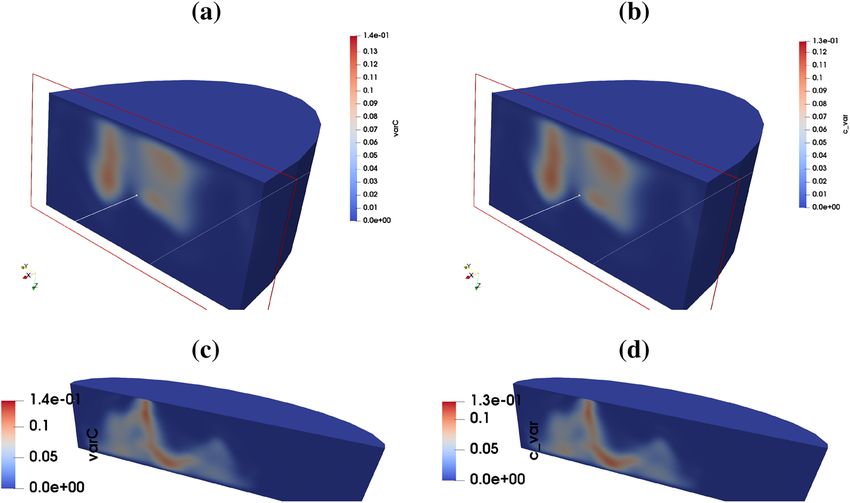
10   Page 2 of 29      GEM - International Journal on Geomathematics   (2020) 11:10

1 Motivation

Accurate prediction of the movement of contamination in groundwater is essential.
Certain pollutants are soluble in water and can leak into groundwater systems, such
as seawater into coastal aquifers or wastewater leaks. Indeed, some pollutants can
change the density of a fluid and induce density-driven flows within the aquifer. This
causes faster propagation of the contamination due to convection. Thus, simulation and
analysis of this density-driven flow play an important role in predicting how pollution
can migrate through an aquifer (Kobus 2000; Fan et al. 1997).
   In contrast to the transport of pollution by molecular diffusion, convection due to
density-driven flow is an unstable process that can undergo quite complicated pat-
terns of distribution. The Elder problem is a simplified but comprehensive model that
describes the intrusion of salt water from a top boundary into an aquifer (Elder 1967a, b;
Voss and Souza 1987; Elder et al. 2017). The evolution of the concentration profile is
typically referred to as fingering. Note that due to the nonlinear nature of the model,
the distribution of the contamination strongly depends on the model parameters, so
that the system may have several stationary solutions (Johannsen 2003).
   Hydrogeological formations typically have a complicated and heterogeneous struc-
ture, and geological media may consist of layers of porous media with different
porosities and permeability coefficients (Schneider et al. 2012; Reiter et al. 2017).
Difficulty in specifying hydrogeological parameters of the media, as well as measur-
ing the position and configuration of the layers, gives rise to certain errors. Typically,
the averaged values of these quantities are used. However, due to the nonlinearities of
the flow model, averaging of the parameters does not necessarily lead to the correct
mathematical solution. Uncertainties arise from various factors, such as inaccurate
measurements of the different parameters and the inability to measure parameters at
each spatial location at any given time. To model the uncertainties, we can use random
variables, random fields, and random processes. However, uncertainties in the input
data spread through the model and make the solution uncertain too. Thus, an accurate
estimation of the output uncertainties is crucial.
   Many techniques are used to investigate the propagation of uncertainties associated
with porosity and permeability into the solution, such as classical Monte Carlo (MC)
sampling. Although MC sampling is dimension-independent, it converges slowly and
therefore requires a lot of samples, and these simulations may be time-consuming and
costly. Alternative, less costly techniques use collocation, sparse grid, and surrogate
methods, each with their advantages and disadvantages. But even advanced techniques
may require hundreds to thousands of simulations and assume a certain smoothness in
the quantity of interest. Our simulations contain up to 4.5 million spatial mesh points
and 1000–3000 time-steps and are therefore run on a massively parallel cluster. Here,
we develop methods that require much fewer simulations, from a few dozen to a few
hundred.
   Perturbation methods, which expand the quantity of interest (QoI) with respect to
random parameters in a Taylor series, were considered and compared in Cremer and
Graf (2015).
   Here, we use the well-established generalized polynomial chaos expansion (gPC )
technique (Xiu and Karniadakis 2002b), where we compute the gPC coefficients by

123
GEM - International Journal on Geomathematics   (2020) 11:10   Page 3 of 29   10

applying a Clenshaw-Curtis quadrature rule (Barthelmann et al. 2000). We use gPC to
compute QoIs such as the mean, the variance, and the exceedance probabilities for
the mass fraction (in this case, a saltwater solution). We validate our obtained results
using the quasi-Monte Carlo (qMC ) approach. Both methods require the computation
of multiple simulations (scenarios) for variable porosity and permeability coefficients.
   To the best of our knowledge, no other reported works have solved the Elder problem
(Voss and Souza 1987; Elder et al. 2017) with uncertain porosity and permeability
parameters using gPC .
   Fingering in a highly unstable free convective flow has been studied in Xie et al.
(2012). Overviews of the uncertainties in modeling groundwater solute transport (Car-
rera 1993) and modeling soil processes (Vereecken et al. 2016) have been performed,
as well as reconnecting stochastic methods with hydrogeological applications (Bode
et al. 2018), which included recommendations for optimization and risk assessment.
Fundamentals of stochastic hydrogeology, an overview of stochastic tools and account-
ing for uncertainty have been described in Rubin (2003).
    Recent advances in uncertainty quantification, probabilistic risk assessment, and
decision-making under uncertainty in hydrogeologic applications have been reviewed
in Tartakovsky (2013), where the author reviewed probabilistic risk assessment
methods in hydrogeology under parametric, geologic, and model uncertainties.
Density-driven vertical transport of saltwater through the freshwater lens has been
modeled in Post and Houben (2017).
   Various methods can be used to compute the desired statistics, such as direct
integration methods (Monte Carlo, quasi Monte Carlo, collocation) and surrogate-
based methods (generalized polynomial chaos approximation, stochastic Galerkin)
(Espig et al. 2014; Matthies and Keese 2005b; Babuška et al. 2004). Direct integra-
tion methods compute statistics by sampling unknown input coefficients (they are
undefined and therefore uncertain) and solving the corresponding PDE, while the
surrogate-based method computes a low-cost functional (polynomial, exponential,
trigonometric) approximation of QoI. Examples of surrogate-based methods include
radial basis functions (Liu and Görtz 2014; Bompard et al. 2010; Loeven et al. 2007;
Giunta et al. 2004), sparse polynomials (Chkifa et al. 2015; Blatman and Sudret 2010),
polynomial chaos expansion (Xiu and Karniadakis 2003; Najm 2009; Conrad and
Marzouk 2013; Xiu 2009; Ghili and Iaccarino 2017) and low-rank tensor approxi-
mation (Dolgov et al. 2015; Kim et al. 2006; Dolgov et al. 2014; Litvinenko et al.
2013; Litvinenko and Matthies 2011). A nonintrusive stochastic Galerkin method was
introduced in Giraldi et al. (2014). The surrogate-based methods have an additional
advantage if gradients are available (Liu et al. 2017). Sparse grid methods to integrate
high-dimensional integrals are considered in Smolyak (1963); Bungartz and Griebel
(2004); Griebel (2006); Klimke (2008); Novak and Ritter (1997, 1996); Gerstner and
Griebel (1998); Novak and Ritter (1999); Conrad and Marzouk (2013); Constantine
et al. (2012); Ghili and Iaccarino (2017). A sparse grid package is available in https://
sparsegrids.org/software/.
    The quantification of uncertainties in stochastic PDEs can pose a great challenge
due to the possibly large number of random variables involved, and the high cost
of each deterministic solution. For problems with a large number of random vari-
ables, the methods based on a regular grid (in stochastic space) are less preferable

                                                                                   123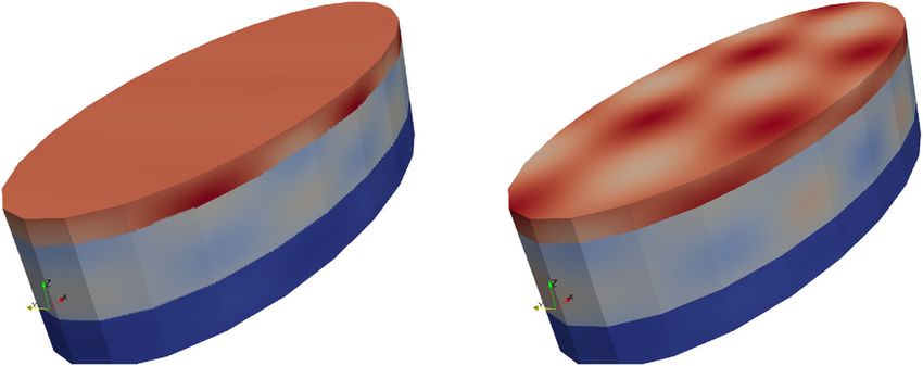
10   Page 4 of 29      GEM - International Journal on Geomathematics   (2020) 11:10

due to the high computational cost. Instead, methods based on a scattered sam-
pling scheme (MC, qMC) give more freedom in choosing the sample number N
and protect against sample failures (i.e., when the numerical code crashes for a given
sample point). The MC quadrature and its variance-reduced variants have dimension-
                                            1
independent convergence with rate O(N − 2 ), and qMC has the worst case convergence
rate O(log M (N )N −1 ), where M is the dimension of the stochastic space (Matthies
2007). Collocations on sparse or full grids are affected by the dimension of the inte-
gration domain (Babuška et al. 2007; Nobile et al. 2015, 2008). In this work, we use
the Halton rule to generate quasi-Monte Carlo quadrature points (Caflisch 1998; Joe
and Kuo 2008). A numerical comparison of other qMC sequences has been described
in Radović et al. (1996).
    The construction of a gPC -based surrogate model Matthies (2007) is similar to com-
puting a Fourier expansion, where only the Fourier coefficients need to be computed.
Some well-known polynomials, such as multivariate Legendre, Hermite, Chebyshev,
and Laguerre functions, are commonly used as a basis Xiu and Karniadakis (2002b).
These expansion functions should possess some useful properties, e.g., orthogonality.
Usually, a small number of quadrature points are used to compute these coefficients.
Once the surrogate is constructed, its sampling can be performed at a lower cost than
a sampling of the original stochastic PDE.
    To tackle the high numerical complexity, we implement a two-level parallelization.
First, we run all available quadrature or sampling points (also referred to as scenarios)
in parallel, with each scenario on a separate computing node. Second, each scenario
is itself computed in parallel on 2–32 cores.
    This work is structured as follows: In Sect. 2, we outline a model of density-driven
groundwater flow in porous media and the numerical methods for this type of problem.
We describe the stochastic modeling, integration methods, and the generalized poly-
nomial chaos expansion technique in Sect. 3. We present details of the parallelization
of the computations in Sect. 4. Our multiple numerical results, described in Sect. 5,
demonstrate the practical performance of the parallelized solver for Elder-type prob-
lems with uncertain coefficients in 3D computational domains. We conclude this work
with a discussion in Sect. 6.

1.1 Our contribution

We applied the gPC expansion to approximate the solution of the density driven flow,
which is modeled by a time-dependent, nonlinear, second order differential equation.
We estimated propagation of input uncertainties in the porosity and permeability into
the mass fraction.

2 Problem setup

2.1 Density-driven groundwater flow

Groundwater in a porous medium such as an aquifer is subject to gravity, and when
there is any spatial variation in groundwater density, a flow will be induced. In this

123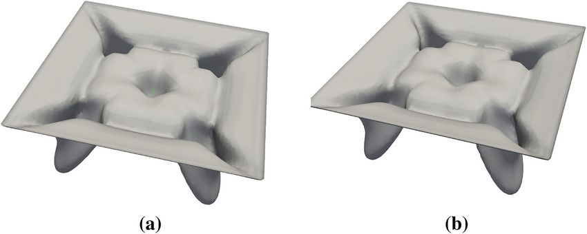
GEM - International Journal on Geomathematics      (2020) 11:10   Page 5 of 29   10

work, we consider an intrusion of saltwater into the aquifer and the dependence of
density on the mass fraction of the dissolved salt. Traditional approaches for modelling
of this system are described in Bear (1972, 1979), Bear and Bachmat (1990), Diersch
and Kolditz (2002), Post and Houben (2017). In this section, we briefly review the
model that we employ.
   We consider a domain D ⊂ Rd , d = 3 that consists of two phases: an immobile
solid porous matrix with a mobile liquid within its pores. We denote the porosity of
the matrix by φ : D → R and its permeability by K : D → Rd×d . The liquid is a
brine solution of N aCl in water. The mass fraction of the brine (saturated saltwater
solution) in the liquid phase is c(t, x) : [0, +∞) × D → [0, 1]. The density of the
liquid phase is ρ = ρ(c) and its viscosity μ = μ(c).
   The motion of the liquid phase through the solid matrix is characterized by the
Darcy velocity q(t, x) : [0, +∞) × D → Rd . Mass conservation of the liquid phase
and the salt can be written as
                              ∂t (φρ) + ∇ · (ρq) = 0,                                   (1)
                              ∂t (φρc) + ∇ · (ρcq − ρD∇c) = 0,                          (2)

where the tensor field D represents molecular diffusion and mechanical dispersion of
the salt. For the velocity q, Darcy’s law is used:
                                                K
                                     q=−          (∇ p − ρg).                           (3)
                                                μ

Here, p = p(t, x) : [0, +∞) × D → R is the hydrodynamic pressure and g =
(0, . . . , −g)T ∈ Rd the acceleration due to gravity.
   In this work, we consider a special case of this general model. We assume that the
porous medium is isotropic and characterized by the scalar permeability K :

    K = K · I, where K = K (x) ∈ R, and I ∈ Rd×d is the identity matrix. (4)

For the density, we set
                                   ρ(c) = ρ0 + (ρ1 − ρ0 )c,                             (5)

where ρ0 and ρ1 are the densities of pure water and the brine, respectively. Note that
c ∈ [0, 1], where c = 0 corresponds to pure water and c = 1 to the fully saturated
solution. The viscosity is assumed to be constant. Finally, dispersion is neglected:

                                           D = φ Dm I,                                  (6)

where Dm is the molecular diffusion coefficient.
   Fields φ(x) and K (x) will depend on the stochastic variables. Values of the other
parameters used in this work are presented in Table 1.
   In our numerical experiments, variants of the Elder problem (Voss and Souza 1987;
Elder et al. 2017) are considered. In the Elder problem, a concentrated solution intrudes
through the upper boundary of an aquifer filled with pure water. Due to the difference in

                                                                                      123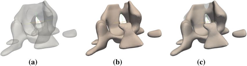
10   Page 6 of 29       GEM - International Journal on Geomathematics     (2020) 11:10

Table 1 Parameters of the density-driven flow problem

Parameters                   Values and units                           Description

φ := E (φ)                   0.1 [–]                                    Mean value of the porosity
Dm                           0.565 · 10−6 [m2 · s−1 ]                   Molecular diffusion
K ref                        4.845 · 10−13 [m2 ]                        Mean value of the permeability
g                            9.81ez [m · s−2 ]                          Gravity
ρ0                           1000 [kg · m−3 ]                           Density of pure water
ρ1                           1200 [kg · m−3 ]                           Density of brine
μ                            10−3 [kg · m−1 · s −1 ]                    Viscosity

densities of the water and the brine, a complicated, unstable flow arises. This leads to a
specific distribution pattern of the intruding solution known as “fingering” (Johannsen
2003). The time evolution of the movement of the brine and the pressure in (1)–(3) is
determined by the initial conditions of c. Note that the system (1)–(3) is nonlinear, and
the model may have several stationary states (Johannsen 2003). Any changes in the
porosity and permeability fields may have a substantial effect on the solution, i.e., the
same initial and boundary data may correspond to fundamentally different asymptotic
behaviors. The influence of this factor can be estimated by applying the stochastic
model.
   In Litvinenko et al. (2019) we considered the same problem with a two-dimensional
reservoir, and in this work we consider two three-dimensional reservoirs: a rectangular
parallelepiped D = [0, 600] × [0, 600] × [0, 150] m3 (Fig. 1a) and an elliptic cylinder
(Fig. 1a) with x ∈ [−300, 300] (the major axis), y ∈ [−150, 150] (the minor axis)
and z ∈ [−150, 0] (the depth). The cylindrical domain is considered to investigate
the influence of the shape on “fingers”. We impose the Dirichlet boundary condition
c = 1 on the red area on the top of D (z = 0), and c = 0 on the green area on the
top and on the other boundaries. For Eq. (1), we impose no-flux boundary conditions
on the bottom and the vertical walls. The boundary conditions for p differ for both
geometries; for the parallelepiped, we impose the no-flux boundary conditions on all
of the boundaries. However, to fix p, we set p = 0 on the edges between the green
and the blue faces. For the cylinder, we set p = 0 on the whole top boundary.
   For the parallelepiped, we try to mimic the standard 2D Elder problem that closes
the upper boundary. In this case, if the pressure is not fixed at any point, it is determined
up to a constant. We fix it and preserve the symmetry of the solution. For the cylinder,
for which the setting is unsymmetric anyway, we model a different situation: We
impose the “atmospheric pressure” on the top, i.e., assume that the top is the surface
of the Earth. Note that these differences are not essential for numerical procedures.
   For the spatial discretization of (1)–(3), we use a vertex-centered finite volume
(FV) scheme. Degrees of freedom (DoFs) for c and p are located in the grid nodes of
the primary mesh. The domain in Fig. 1a is covered by a grid of 524,288 hexahedra,
so that the total number of the DoFs is 1,098,306. For the domain in Fig. 1b, we use
an unstructured mesh of 241,152 tetrahedra with 89,586 DoFs.
   The resolution of the spatial and temporal discretizations play an important role in
the accuracy of the simulations. The distribution of the hydrogeological parameters

123

GEM - International Journal on Geomathematics      (2020) 11:10          Page 7 of 29    10

Fig. 1 a Rectangular parallelepiped D = [0, 600]×[0, 600]×[0, 150] m3 and b elliptic cylindrical domain
with x ∈ [−300, 300] (the long side), y ∈ [−150, 150] (the short side) and z ∈ [−150, 0] (the depth) used
in 3D simulations

of the porous medium should be represented correctly. Moreover, smoothing the flow
on a coarse grid due to numerical diffusion can lead to a loss of some phenomena and
therefore reduce the accuracy of the uncertainty quantification. To this end, we tested
the grid convergence of the simulations with respect to the spatial mesh. We ran our
simulation on the twice regularly refined spatial mesh for geometry from Fig. 1b. The
domain consisted of 15,433,728 cells and has 2,822,552 DoFs. The obtained solution
was similar to the solution, computed on the coarser mesh mentioned above. Thus,
further refinement essentially does not change the behaviour of the solution.

2.2 Stochastic modeling of porosity, permeability and mass fraction

In the model (1)–(3), there are two essential hydrogeological parameters, the porosity φ
and the permeability K, that depend on the spatial coordinates. In general, φ and K are
completely unknown or known (measured) only in a few locations. These coefficients
could be very complicated (discontinuous, jumping, multiscale).
    One of the approaches to deal with such unknown or incomplete data is to extrapo-
late known measurements to the whole domain (Nowak and Litvinenko 2013). Another
approach is to use random fields for modeling φ and K (Ghanem and Spanos 1991;
Keese and Mattthies 2005). The Karhunen–Loève expansion (KLE) is used to approx-
imate these fields. In the KLE approach it is assumed that the covariance matrices of φ
and K are given. Or, alternatively, these covariance matrices could be estimated from
the available data. Then, an auxiliary eigenvalue problem (Khoromskij et al. 2009),
where the covariance function is the kernel of a certain integral operator (Ghanem
and Spanos 1991; Karhunen 1946), is solved. The solution of this eigenvalue prob-
lem builds the KLE expansion, which represents the random field φ (and K). This
is a very well established approach, (cf. Schwab and Todor 2006, 2003; Ghanem
and Spanos 1991). In this work, to avoid a very expensive solution of the eigenvalue
problem (which is a very non-trivial task in large domains, distributed over many
computational nodes), we directly write:

                                                                                              123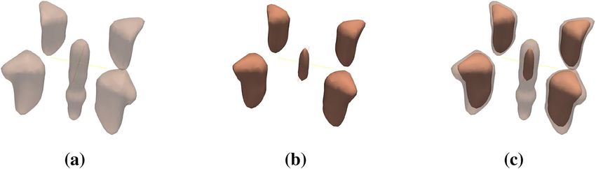
10   Page 8 of 29      GEM - International Journal on Geomathematics    (2020) 11:10


                                                  K
                       φ(x, θ (ω)) = ϕ0 (x) +            ϕi (x)θi (ω),                  (7)
                                                   i=1

where ϕ0 (x) is a deterministic part, {ϕi (x)}i=1K functions, which emulate a basis in

L 2 (D), and θi random variables. Note, that the constructed expansion is not the
Karhunen–Loève expansion. Approximating the covariance operator and computing
the KLE is beyond the scope of this work. If a parallel eigenvalue solver is on hand,
then it could be integrated with our software library, and more realistic expansions
(truncated KLE) could be used instead of our simplified models [see, e.g., (27), (28)].
    Another approach to deal with uncertainties in the porosity and permeability is to
introduce a prior statistical distribution for both and then use the Bayesian (or similar)
updating techniques (Rosić et al. 2013; Matthies et al. 2016) to construct the posterior
distribution.
    To reduce the total numerical complexity, we consider a simplified model, where
the permeability is a non-linear function of the porosity. Particularly, the same random
variables are used for modeling both coefficients. Some empirical and theoretical laws
connecting porosity and permeability have been proposed in the literature (Panda and
Lake 1994; Pape et al. 1999; Costa 2006). In the following, we model the porosity
(φ(x)) by a random field (φ(x, θ )) and assume that the permeability K, cf. (4), is a
non-linear function of φ:

                                      K = K (φ)I.                                       (8)

In our experiments, we use a Kozeny–Carman-like dependence (Costa 2006):

                                                    φ3
                                K (φ) = κ K C ·          ,                              (9)
                                                  1 − φ2

where the scaling factor κ K C is chosen to satisfy the equality K (φ) = K ref , i.e.,
               2
        1−φ
κK C =       3
                 · K ref . Here K ref is a given value. K ref and other parameters of the
           φ
standard Elder problem are listed in Table 1. Since φ and K are uncertain, the solution
c(φ, K) is uncertain too.
Remark 1 Establishing a relationship between porosity and permeability requires
assumptions on the structure of the porous medium in the aquifer. Introducing addi-
tional random variables for the permeability would significantly increase the size of
the problem and restrict the possibility to perform numerical tests, and at the same time
would not principally change the method. For this reason, we used the same random
variables for both.
Remark 2 The Kozeny–Carman model is simple, but it models the essential phenom-
ena for our numerical tests. It introduces a non-linear relation between permeability
and porosity so that the equations cannot be merely re-scaled. This underlines the non-
linear nature of the dependence of the solution (the mass fraction) on these parameters.
From this point of view, the Kozeny–Carman law is non-trivial enough for our purpose.

123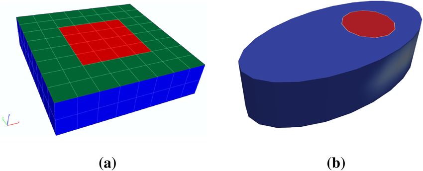
GEM - International Journal on Geomathematics       (2020) 11:10         Page 9 of 29      10

2.3 Solution of the deterministic problem

We start with sampling random variables {θ i } and computing the realizations of poros-
ity φi (x) = φ(x, θ i ) [as in (7)] and then permeability Ki (x) = K(x, θ i ). For this data,
we solve the system of equations (1)–(2). They are discretized by a vertex-centered
finite-volume method on unstructured grids, as presented in Frolkovič (1998). In par-
ticular, we used the consistent velocity approach for the approximation of the Darcy
velocity (3), (Frolkovič 1998; Frolkovič and Knabner 1996). The implicit Euler scheme
for the time discretization was used. The choice of the implicit time-stepping scheme
is motivated its unconditional stability, as the velocity depends on the unknowns of the
system. This is especially important for variable coefficients as it is difficult to predict
the range of the variation of the velocity in the realizations.
   The discretization yields a large sparse system of nonlinear algebraic equations in
every time step. We solve it using the Newton iteration with a line search method. The
sparse linear system appearing in the nonlinear iterations is solved by the BiCGStab
method (Zhaojun et al. 2000) with the geometric multigrid preconditioning [V-cycle,
(Hackbusch 1985)], which proved to be very efficient in this case. On the multigrid
cycle, we used the ILUβ -smoothers (Hackbusch 1994).

3 Stochastic modeling and methods

Let θ = (θ1 , . . . , θ M ) be a vector of independent random variables. Let S := (Θ, B, P)
be a probability space. Here Θ denotes a sample space, B a σ -algebra on Θ, and P a
probability measure on (Θ, B). The solution c(t, x, θ ) lies in the tensor product space
L 2 (D) ⊗ L 2 (Θ) ⊗ L 2 ([0, T ]), where [0, T ] is a time interval, on which the initial
value problem is solved. After discretization, we obtain c ∈ Rn ⊗ R|J | ⊗ Rn t , where n
is the number of basis functions in the physical space, |J | dimension of the stochastic
space, and n t the number of time steps.

3.1 Sampling methods

Well-known methods to estimate the mean and the variance are sampling methods,
such as the quasi-Monte Carlo, Monte Carlo, collocation, and sparse grid methods.
The empirical mean value and the variance of c(t, x, θ ) can be computed as follows

                                                                      Nq

          c(t, x) = E (c(t, x, θ )) =           c(t, x, θ ) P(dθ ) ≈         wi c(t, x, θ i ),    (10)
                                            Θ                          i=1

with Nq quadrature points θ i and weights wi . Here, c(t, x, θ i ) is the solution evaluated
at a fixed point θ = θ i ∈ R M . The sample variance is computed as follows

                                         Nq

                      Var[c](t, x) ≈            wi (c(t, x) − c(t, x, θ i ))2 .                   (11)
                                         i=1

                                                                                                 123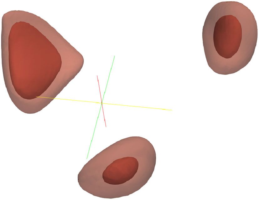
10   Page 10 of 29      GEM - International Journal on Geomathematics   (2020) 11:10

3.2 (Generalized) polynomial chaos expansion

The dependence of the uncertain physical quantities (the solution of the PDE, or QoI)
on random variable θ : Θ → R M can be represented in terms of the (generalized)
polynomial chaos expansion (Wiener 1938). Here we require that this physical quantity
has a finite variance. Different orthogonal polynomials (Hermite, Legendre, Cheby-
shev, Laguerre) (Askey and Wilson 1985; Xiu and Karniadakis 2002b, 2003; Sudret
2008), or splines, can be used.
   To introduce polynomial expansions, we, first, need to introduce the notions of
multiindex and multiindex sets. Let β be a multi-index
                                                                 (N)
                         β = (β1 , . . . , β j , . . .) ∈ J := N0 ,                     (12)

and J is a multiindex set, containing sequences of non-negative integers. We assume
{Ψβ }β∈J is a multivariate basis of S = L 2 (Θ, B, P). The cardinality of the multi-index
set J is infinite.
   Polynomial chaos expansion (PCE) was introduced in Wiener (1938). It was shown
[Cameron and Martin theorem (Cameron and Martin 1947)], that if c(θ ) is a second-
order random variable (a function in L 2 (Θ)), then it can be expanded as follows:

                                  c(θ) =          cβ Ψβ (θ ).                           (13)
                                            β∈J

This expansion converges in the L 2 (Θ) sense. Here {Ψβ } are multivariate Hermite
polynomials of multi-dimensional Gaussian random variables (θ). The advantage of
PCE is that from this point we may forget the original probability space and only work
with (Θ, Γ ) with a Gaussian measure.
Definition 1 For numerical computations, the infinite series above can be truncated,
i.e., we keep only M random variables, θ = (θ1 , . . . , θ M ), and limit the total degree
of the multi-variate polynomial Ψβ (θ ) by P. We denote the new multiindex subset as
J M,P ⊂ J .
    The truncated multi-index set is defined by restricting the sum of components,

          J M,P := {α = (α1 , . . . , α M ) :     α ≥ 0, α1 + · · · + α M ≤ P} .

The truncated set contains (M+P)!
                            P!M! values. This may become a enormous number even
for small P and M. Another approach is to preselect the set of polynomials with the
moderate cardinality (Todor and Schwab 2007; Matthies and Keese 2005b; Blatman
and Sudret 2010; Chkifa et al. 2015).
   The expansion (13) can be extended for time-dependent random fields:

                            c(t, x, θ ) =         cβ (t, x)Ψβ (θ),
                                            β∈J

where coefficients cβ (t, x) depend on t and x. For representing of more general, non-
Gaussian fields/processes, the generalized polynomial chaos (gPC ) expansion (Xiu

123
GEM - International Journal on Geomathematics (2020) 11:10 Page 11 of 29 10
and Karniadakis 2002b; Xiu 2010; Xiu and Karniadakis 2002a) was introduced. In
gPC , instead of Hermite orthogonal polynomials, other orthogonal polynomials can
be used [(see more in the Appendix or in Xiu and Karniadakis (2002b), Xiu and Karni-
adakis (2003), Ernst et al. (2012)]. Utilization of other types of orthogonal polynomials
could result in a more efficient expansion with a smaller number of terms. In this work,
we use multivariate Lagrange polynomials with uniform RVs θ . The correspondence
between the type of gPC and their underlying random variables is shown in Table 5.1 in
Xiu (2010) (the Wiener–Askey scheme). The optimal (exponential) convergence rate
of each Wiener–Askey polynomial chaos expansion was numerically demonstrated in
Xiu and Karniadakis (2002b).
3.3 Truncated (generalized) polynomial chaos expansion
For numerical purposes, we truncate the infinite gPC series above and obtain
c(t, x, θ ) ≈
c(t, x, Θ) = cβ (t, x)Ψβ (θ). (14)
β∈J M,P
Here, Ψβ (θ ) are multi-variate Legendre polynomials defined as follows
M
M
Ψβ (θ ) := ψβ j (θ j ); ∀θ ∈ R M , β ∈ J M,P , β j ≤ P,
j=1 j=1
ψβ j (·) are univariate Legendre polynomials, defined in (30). The scalar product on
L 2 (Θ) is
Ψα , Ψβ L 2 (Θ) = E Ψα (θ )Ψβ (θ ) = Ψα (θ )Ψβ (θ )dPθ = Q α δαβ , (15)
Θ
where Q α = E Ψα2 = qα1 · · · qα M , qα j = ψα j , ψα j = 1/(2α j + 1), are the
normalization constants and δαβ = δα1 β1 · · · δα M β M is the M-dimensional Kronecker
delta function.
Example 1 Let M = 3 and the maximal polynomial degree be P = 2. Then the mul-
tiindex β is β = (β1 , β2 , β3 ), and the multiindex set contains the following elements
J3,2 : = {(0, 0, 0), (1, 0, 0), (0, 1, 0), (0, 0, 1), (2, 0, 0), (16)
(1, 1, 0), (1, 0, 1), (0, 2, 0), (0, 1, 1), (0, 0, 2)}. (17)
Remark 3 The mass fraction c is scaled to take value in [0, 1]. The gPC approximation
(14) of the mass fraction may take negative values or values larger than 1. A possible
remedy is to assume that c can be written as exp(γ ), where γ varies from −∞ to +∞,
and then approximate the auxiliary function γ = log c instead of the mass fraction
itself:
12310 Page 12 of 29 GEM - International Journal on Geomathematics (2020) 11:10
γ (t, x, θ ) = γβ (t, x)Ψβ (θ). (18)
β∈J
We also note that the trick with the log function does not prevent c from taking values
larger than 1. Keeping c ≤ 1 can be achieved by approximating another transformed
variable, like the scaled arctan. Another function that can be used is the error-function
erf (this is sometimes called a “probit” approximation), or the logistic function (called
“logit”). In this work, for the sake of simplicity, we did not change the variables. We
were lucky that in the settings we used (small variance in the input parameters), we
did not observe negative c (or c > 1). But for the future, we strongly recommend
doing such changes of variables.
Decomposition (14) can be understood as a response surface for c(t, x, θ ). As soon
as the response surface is built, the value c(t, x, θ ) can be evaluated for any θ almost
for free (without further solutions the groundwater flow PDE). It can be very practical
if 106 samples of c(t, x, θ ) are needed, for example. Since {Ψβ } polynomials are
L 2 -orthogonal, the coefficients cβ (t, x) can be computed by projection:
Nq
1 1
cβ (t, x) =
c(t, x, θ )Ψβ (θ) P(dθ ) ≈ Ψβ (θ i )
c(t, x, θ i )wi ,
Ψβ , Ψβ Θ Ψβ , Ψβ
i=1
where wi are weights and θ i quadrature points, defined, for instance, by a Clenshaw-
Curtis integration rule. Once all gPC coefficients are computed, we can compute the
required statistics. For estimates of truncation and aliasing errors, see Conrad and
Marzouk (2013), Ghili and Iaccarino (2017).
Possible ways to apply dimensionality reduction on PCE in the spirit of the Basis
Adaptation techniques are considered in Tipireddy and Ghanem (2014), Tsilifis et al.
(2019), Thimmisetty et al. (2017), Tsilifis and Ghanem (2018).
Remark 4 If only the variance and the mean values are of interest, we recommend
using the collocation method with some sparse or full-tensor grid. If some additional
statistics are required, such as sensitivity analysis (Sudret 2008; Crestaux et al. 2009),
parameter identification, or computing cdf or pdf, we recommend computing the gPC
expansion.
Quadrature grids for computing multi-dimensional integrals can be constructed
from products of 1D integration rules. To keep computational costs to a minimum, a
sparse grid technique can be used for certain classes of smooth functions (Bungartz
and Griebel 2004).
Since Ψ0 (θ ) ≡ 1, it becomes apparent that the mean value is the first gPC coefficient
1
c(t, x) := E (c(t, x, θ )) = c0 (t, x) = c(t, x, θ )Ψ0 (θ) P(dθ )
Ψ0 , Ψ0 Θ
Nq
≈ c(t, x, θ i )wi , (19)
i=1
123GEM - International Journal on Geomathematics (2020) 11:10 Page 13 of 29 10
0 = (0, . . . , 0). The variance is the sum of squared gPC coefficients (Xiu and Karni-
adakis 2002b; Ghanem et al. 2017; Le Maître and Knio 2010):
Var[c](t, x) = Var[c(t, x, θ )] = E (c(t, x, θ ) − c)2 (20)
= Ψγ 2 cγ (t, x) ⊗ cγ (t, x)
γ >0
M
1
= cγ (t, x)2 . (21)
2γk + 1
γ >0 k=1
3.4 Computing probability density functions
Once we have calculated the gPC surrogate c(t, x, θ ) in (14), we can approximate the
probability density functions (see Fig. 10), exceedance probabilities and quantiles in
the selected points. For this, we should evaluate the multi-variate polynomial c(t, x, θ )
in a sufficiently large number of points θ
c(t ∗ , x∗ , θ ) =
c(θ ) := cβ (t ∗ , x∗ )Ψβ (θ ). (22)
β∈J M,P
The random variable c(θ ) can be sampled, e.g., Ns = 106 times (no additional exten-
sive simulations are required). The obtained sample can be used to evaluate the required
statistics and the probability density function. The exceedance probability for some
threshold c∗ can be estimated as follows:
c(θ i ) > c∗ , i = 1, . . . , Ns }
c(θ i ) :
#{
Prob(c > c∗ ) ≈ . (23)
Ns
Having a sufficiently large sample set makes it possible to estimate quantiles Litvi-
nenko et al. (2019).
3.5 Approximation and truncation errors
Applying gPC approximation, will introduce truncation and approximation errors
(Constantine et al. 2012; Sinsbeck and Nowak 2015; Conrad and Marzouk 2013;
Ghili and Iaccarino 2017; Ernst et al. 2012). By truncating gPC coefficients {cβ : β ∈
J \ J M,P }, we introduce the truncation error in the L 2 (Θ) norm
errtr = c(t, x, θ ) −
c(t, x, θ ) L 2 (Θ) = cβ (t, x)Ψβ (θ ) (24)
L 2 (Θ)
β∈J \J M,P
In further numerical experiments we average the error over Θ, i.e., compute the
error as a function of time and space errtr := errtr (t, x). Additionally, we approximate
the coefficients cβ (t, x) by
cβ (t, x). This introduces the approximation error
12310 Page 14 of 29 GEM - International Journal on Geomathematics (2020) 11:10
erra = cβ (t, x)Ψβ (θ) −
cβ (t, x)Ψβ (θ )
L 2 (Θ)
β∈J M,P β∈J M,P
= (
cβ (t, x) − cβ (t, x))Ψβ (θ) (25)
L 2 (Θ)
β∈J M,P
The sum of both errors is
errtr + erra = cβ (t, x)Ψβ (θ )
L 2 (Θ)
β∈J \J M,P
truncation error
+ (cβ (t, x) −
cβ (t, x))Ψβ (θ) . (26)
L 2 (Θ)
β∈J M,P
approximation error
Remark 5 Spatial resolution plays a vital role in the simulations. Thus, the distribution
of the parameters of the porous medium should be represented correctly. Furthermore,
smoothing the flow on a coarse grid due to numerical diffusion can lead to a loss of
some phenomena and therefore reduce the accuracy of the uncertainty quantification.
Thus, we must cover D with sufficiently fine grids and use sufficiently small time
steps.
4 Parallelisation
Because of the massive numerical complexity of the problem, all computations were
performed on a Cray XC40 parallel cluster Shaheen II provided by King Abdullah
University of Science and Technology (KAUST) in Saudi Arabia (https://www.hpc.
kaust.edu.sa/content/shaheen-ii). Shaheen II has 6174 nodes with 2 Intel Haswell 2.3
GHz CPUs per node, and 16 processor cores per CPU. Every node has 128 GB RAM.
The nodes communicate via the Cray Aries interconnect network with Dragonfly
topology. The system is equipped with the Sonexion Lustre 2000 storage appliance.
There are two levels of parallelism in our implementation. On the top level, we
compute all scenarios in parallel. Each scenario corresponds to a particular quadrature
or collocation point in the stochastic space. For every scenario, a separate node of
the cluster is allocated. All scenarios are independent, so there is no communication
between the nodes. We allocate, depending on the experiment, up to 600 computing
nodes. This allows us to compute (up to) 600 qMC (or quadrature) simulations simul-
taneously. Shaheen II uses the SLURM system to manage parallel jobs, and we used
the SLURM job arrays for the concurrent computations of the scenarios.
On the bottom layer, computation of each single scenario (one quadrature point) is
done in parallel on the 32 cores of one node. This parallelisation is based on the distri-
bution of the discretization grid between the processes and the communication using
MPI. As this happens on the cores of one node, the network hardware is not involved.
This part is implemented in ug4 . The parallel efficiency of this toolbox for solving
123GEM - International Journal on Geomathematics (2020) 11:10 Page 15 of 29 10
two- and three- dimensional Laplace problems is analyzed in Reiter et al. (2013). The
scalability of ug4 in the case of the 2D Elder problem is presented (Vogel et al. 2013).
Also, the speedup in these computations cannot be ideal (due to the communication);
the toolbox demonstrates very high efficiency for this type of problem. We refer also
to Heppner et al. (2013), Vogel (2014) for further details.
Thus, in total, we run our code on up to 600×32 = 19200 parallel cores. Depending
on the grid step sizes the total computing time could be up to 24 h.
The computations of the mean value, variance, and other statistics are done in the
postprocessing phase in parallel on all cores of only one node. Herewith the same
distribution of the spatial grid, as for the computation of each realization, is used.
The spatial grid is distributed between the cores of that single node, and its parts are
processed concurrently. No communication between the processes is required, and the
computation of the statistics takes a very short time in comparison with the computing
all scenarios.
5 Numerical experiments
5.1 Software
To compute the deterministic solutions, we used d3 f plugin of the simulation frame-
work ug4 (Reiter et al. 2013; Vogel et al. 2013). ug4 is a novel flexible software system
for simulating PDE based models on high performance parallel clusters. It is capable
of numerical treatment of non-stationary non-linear systems of PDEs. This software
framework has successfully been applied to a variety of problems such as density-
driven and thermohaline flow in porous media, the Navier–Stokes equations, drug
diffusion through human skin, and level-set methods. Special care is given to parallel
performance issues, scalability, linear algebra algorithms, and data structures. In addi-
tion, ug4 is specially designed for user-friendly handling and functionality is made
available to non-programming users through the scripts and graphical representations.
5.2 3D computational domains
The geometry of real-life 3D computational domains can be very complicated. Dis-
cretization of such domains (reservoirs) may require non-trivial 3D meshes. This
can be very challenging in the stochastic context, such as we have here. There-
fore, we start with two relatively trivial reservoir geometries: (1) a parallelepiped
D = [0, 600] × [0, 600] × [0, 150] (see Fig. 1a); (2) an elliptic cylinder with the
semi-axes 600 and 300 for the base ellipse and height 150. Thus, the longest radius
is 300, x ∈ [−300, 300], the shortest radius is 150, y ∈ [−150, 150], the height
z ∈ [−150, 0] and the center is in the point (0, 0, −75) (see Fig. 1b). The polluted
area is a circle with the center in (−150, 0, 0), and with radius 100.
12310 Page 16 of 29 GEM - International Journal on Geomathematics (2020) 11:10
5.3 Parallelepiped with 3 RVs
For every realization, the porosity and permeability are functions of the spatial coor-
dinates. These functions can be expanded into the Fourier series that would introduce
the sine and cosine functions. Therefore, in (27) and (28), we used the sine and cosine
functions to model the in-homogeneity of the medium. Note that a natural assumption
for the Darcy flow would be that the expansion is finite, i.e., high-frequency modes
are truncated. The suggested model is homogenized and does not resolve the scales
of the pores. With the current state of the computational equipment, we had to con-
fine ourselves with only a few Fourier modes. Besides that, we used linear factors to
introduce some global variation in the porosity.
In the following, we consider an experiment with three random variables θ =
(θ1 , θ2 , θ3 ) and with the following porosity coefficient
xπ yπ zπ xπ yπ
φ(x, θ ) := 0.1 + 0.01 θ1 sin + θ2 sin + θ3 sin + θ1 sin sin
600 600 150 600 600
xπ zπ
+ θ2 sin sin , (27)
600 150
where x = (x, y, z) ∈ [0, 600] × [0, 600] × [0, 150] (parallelepiped). With this
porosity coefficient we try to model the inhomogeneity of the medium. For every
realization, the porosity and the permeability are functions of the spatial coordinates.
In general, φ(x, θ ) can be expanded into the Fourier series that would introduce the
sine and cosine functions. Note that a natural assumption for the Darcy flow would
be that the expansion is finite, i.e., high-frequency modes are truncated. The model
is homogenized and does not resolve the scales of the pores. Surely, with the current
state of the computational equipment, we had to confine ourselves with only a few
Fourier modes.
In Fig. 2, we visualize isosurfaces E (c) = 0.5 after 1500 time steps of length
0.005 years, computed using (a) 200 qMC simulations (Halton sequence) and (b)
gPC response surface of total degree P = 4. All gPC coefficients were computed via
a 3D quadrature rule with 125 quadrature points. In our numerical experiments with
the polynomial degrees P < 4 we were not able to compute the variance accurately.
Note that in the present problem setting, the flow field is very complicated. The main
process tends to represent the same behaviour as in the 2D version of the Elder problem
(Litvinenko et al. 2019). The highly concentrated solution from the top boundary
moves downward and displaces the pure water located initially at the bottom. This
pure water is pushed up. As the diffusion is very small, the transport of the salt by
these opposite flows creates a non-trivial pattern of the concentration field, typically
described as “fingering”. The particular pattern depends on the profile of the boundary
conditions for c and the initial flow. In our case, we see 5 “fingers” (4 at the corners
and one at the center). As we see, the isosurfaces of E (c) = 0.5 are almost identical
for both methods.
The same holds for the variance. Figure 3 presents the isosurface Var[c] = 0.05
after 1500 time steps for (a) 200 qMC simulations (Halton sequence), (b) gPC response
surface of degree 4 and (c) comparison of the isosurfaces from (a) and (b). We see that
123GEM - International Journal on Geomathematics (2020) 11:10 Page 17 of 29 10
Fig. 2 Isosurface E (c) = 0.5 computed using a 200 qMC simulations and b gPC response surface of
degree 4. The upper square edge corresponds to the boundary of the red area in Fig. 1a
Fig. 3 Isosurface Var[c] = 0.05, computed via a qMC and b gPC response surface of degree 4, and c
comparison of both isosurfaces
positions, numbers, and shapes of all the fingers are similar. The isosurfaces, computed
via qMC , are slightly larger, especially the one in the middle (see Fig. 3c).
Five different contour lines (isosurfaces) of the deterministic solution c(x, θ = 0)
for the porosity, defined in (27), are shown in Fig. 4.
5.4 Elliptical cylinder with 3 RVs
In this example we consider a cylindrical domain (see Fig. 1b). The goal is to see the
influence of the computing domain on the solution. Indeed, as we can see below, the
number of fingers and their shapes are different.
The porosity coefficient has three layers and is defined with three RVs as follows:
θ1 x πx πy πx πy
φ(t, x, θ ) = 0.1 + 0.05 · c0 · cos + θ2 sin + θ3 cos sin
600 300 150 300 150
(28)
c0 = 0.01 if z ≤ −100
c0 = 0.10 if −100 < z ≤ −50 (29)
c0 = 1.0 if −50 < z ≤ 0
12310 Page 18 of 29 GEM - International Journal on Geomathematics (2020) 11:10
Fig. 4 Five isosurfaces of the deterministic solution c(t, x, θ = 0) = {1.0, 0.75, 0.5, 0.25, 0.0} after 9.6
years; a view from the top; b view from the bottom. The upper square edge corresponds to the boundary of
the red area in Fig. 1a
Fig. 5 Two realizations of the porosity field, φ(x) ∈ [0.079, 0.13]
Figure 5 shows two random realizations of the porosity field.
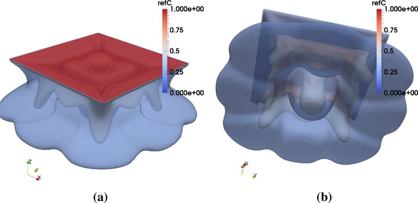
In Fig. 6 we present a comparison of the variance of c, computed via qMC (200
simulations) and gPC of degree P = 4. All (M+P)!
M!P! = 3!4! =35 gPC coefficients are
7!
computed with a full Clenshaw–Curtis quadrature Clenshaw and Curtis (1960), con-
taining 125 quadrature points. In Fig. 6a and b the cutting plane has the normal
vector (1, 0, 0), and Fig. 6c and d have the normal vector (0, 1, 0). The variances,
computed via qMC and gPC , lie in the intervals Var[c]q MC ∈ [0, 0.14], and
Var[c]g PC ∈ [0, 0.13] respectively. The small difference is not really visible in the
pictures. Thus, we conclude that the gPC surrogate model, computed on a Clenshaw-
Curtis quadrature grid, can be used for approximating the mean and the variance of
c.
To demonstrate more similarities between the solutions, computed via qMC and
gPC , we visualize isosurfaces of the variance of the mass fraction in the cylindrical
3D reservoir (Figs. 7 and 8). In Fig. 7 we demonstrate two isosurfaces Var[c] = 0.025
computed via a) qMC method, and b) gPC of degree 4 surrogate. Figure 7c shows the
123GEM - International Journal on Geomathematics (2020) 11:10 Page 19 of 29 10
Fig. 6 Variance of the mass fraction in the cylindrical 3D reservoir, computed via 200 qMC simulations (a)
and (c); and gPC of degree 4 with 35 gPC coefficients (b) and (d). Var[c]q MC ∈ [0, 0.14], Var[c]g PC ∈
[0, 0.13]. The first cutting plane on a–b has normal vector (1, 0, 0), the second on c–d (0, 1, 0)
Fig. 7 The contour Var[c] = 0.025, computed by a qMC , b gPC and c comparison of both
comparison of both isosurfaces. The results are very similar, although the isosurface
computed via gPC is slightly larger.
In Figure 8 we demonstrate two isosurfaces Var[c] = 0.07 computed via a)
qMC method (Fig. 8a, and b) gPC of degree 4 (Fig. 8b). Figure 8c shows the compar-
ison of both isosurfaces. Again, the results are very similar, and it is hard to say which
isosurface is “larger” or “smaller”.
In Fig. 9 we compare two isosurfaces Var[c] = 0.12 computed via (1) qMC method
and (b) gPC of degree 4. Once again, the results (the number of fingers and their shape)
are very similar. The isosurface computed via qMC is slightly larger.
In Fig. 10 (left) and (right) we compare four pdfs, computed with polynomial
degrees P = {1, 2, 3, 4}, M = 3, in two fixed points (100, 0, −50) (left) and
(100, 0, −25) (right) in the cylindrical domain, after T = 400 time steps (each step is
equal to 0.006 years). We can see that P = {2, 3, 4} are giving approximately equal
12310 Page 20 of 29 GEM - International Journal on Geomathematics (2020) 11:10
Fig. 8 Isosurface Var[c] = 0.07, computed via a qMC and b gPC response surface of degree 4, and c
comparison of both isosurfaces
Fig. 9 Comparison of
isosurfaces Var[c] = 0.12,
computed via qMC and
gPC response surface of degree
4. The isosurface computed via
qMC is slightly larger
Fig. 10 Comparison of four pdfs, computed with polynomial degrees P = {1, 2, 3, 4}, M = 3, in two
different points (100, 0, −50) (left) and (100, 0, −25) (right) in the cylindrical domain, after T = 400 time
steps (each step is equal to 0.006 years)
results for both points (t, x). The variance for P = {3, 4} is slightly smaller as the
variance for P = 2. The exact value of c is unknown, and the deterministic value of
c at (100, 0, −50) is 0.8, and at (100, 0, −25) is 0.995.
123GEM - International Journal on Geomathematics (2020) 11:10 Page 21 of 29 10
Fig. 11 Propagation of the mean of the mass fraction in the cylindrical 3D reservoir, cutting plane is
(150, y, z). Evolution of E (c) in time after a 0, b 0.55, c 1.1, d 2.2 years
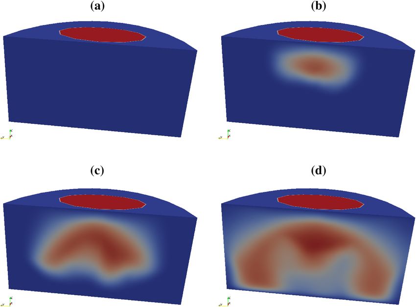
Fig. 12 Propagation of the variance of the mass fraction in the cylindrical 3D reservoir, cutting plane is
(150, y, z). Evolution of Var[c](t, x) in time after a 0.55, b 1.1, c 2.2 years (100, 200, 400 time steps
respectively). After 400 time steps Var[c] ∈ [0, 0.17]
5.5 Time evolution of c(t, x) and Var[c](t, x)
Here we repeat the experiment with φ as in (28)–(29). The gPC coefficients were
computed with 125 quadrature points. Figure 11 shows the evolution of the mean of
the mass fraction in the cylindrical 3D reservoir after (a) 0, (b) 0.55, (c) 1.1, (d) 2.2
years. The cutting plane is (150, y, z). The different stages of the fingers building over
time are clearly visible.
Figure 12 shows the variance of the mass fraction in the cylindrical 3D reservoir
after {0.55, 1.1, 2.2} years (after 100, 200, and 400 time steps, respectively).
12310 Page 22 of 29 GEM - International Journal on Geomathematics (2020) 11:10 5.6 Best practices After numerous numerical tests, we created a best practice guide as outlined below: 1. The number of uncertain variables describing the porosity coefficient depends on the model and assumptions. We recommend to start with 1–3 variables to improve understanding of the phenomena . We note that a heterogeneous porosity field in 3D may require hundreds of random variables. That can mean thousands of gPC coefficients. This is computationally unaffordable unless we use some advanced low-rank tensor techniques (Dolgov et al. 2014) or multi- scale/homogenization strategy. In this work, we considered three random variables. The more random variables that are present, the harder it can be to interpret the results, and additional sensitivity analysis (Sudret 2008; Crestaux et al. 2009) may be required. 2. We assume a smooth dependence of the output QoI on the uncertain input param- eters. We recommend to check it at least visually before computing gPC . 3. The gPC -based surrogate, for the cases when the variance of the porosity is not so high, showed reliable results. For the validation, a qMC method can be used. 4. We were unable to achieve a correct variance of c with the gPC method in tests where the variance of the porosity was large. 5. We recommend the total polynomial degree in gPC to be P = 4 or 5. With our computational budget, we failed to get the correct variance of c for P > 5. Addi- tionally, the quadrature rule was probably not robust enough to catch the oscillatory behavior of the gPC polynomials. This is a known drawback of using global poly- nomials. 6. The coefficients of the gPC surrogate require calculating high-dimensional inte- grals. It could be hard to compute small gPC coefficients. As a result, it could be hard to compute the variance accurately. 7. The total numerical cost could be reduced by choosing adaptive spatial and time step sizes, depending on the random perturbation (the Multi level Monte Carlo or Multi-index Monte Carlo methods). But we also observed that a large time or spatial step sizes may result in a lack of convergence. 6 Conclusion In this work, we solved the density driven groundwater flow problem with uncertain porosity and permeability. An accurate solution of this time-dependent and non-linear problem is impossible because of the presence of natural uncertainties in the reservoir such as porosity and permeability. Therefore, we estimated the mean value and the variance of the solution, as well as the propagation of uncertainties from the random input parameters to the solution. We started by defining the Elder-like problem. Then we described the multi- variate polynomial approximation (gPC ) approach and used it to estimate the required statistics of the mass fraction. Utilizing the gPC method allowed us to reduce the com- putational cost compared to the classical quasi Monte Carlo method. gPC assumes 123
GEM - International Journal on Geomathematics   (2020) 11:10   Page 23 of 29   10

that the output function c(t, x, θ ) is square-integrable and smooth w.r.t uncertain input
variables θ .
    Many factors, such as non-linearity, multiple solutions, multiple stationary states,
time dependence and complicated solvers, make the investigation of the convergence
of the gPC method a non-trivial task.
    We used an easy-to-implement, but only sub-optimal gPC technique to quantify
the uncertainty. For example, it is known that by increasing the degree of global
polynomials (Hermite, Langange and similar), Runge’s phenomenon appears. Here,
probably local polynomials, splines or their mixtures would be better. Additionally,
we used an easy-to-parallelise quadrature rule, which was also only suboptimal. For
instance, adaptive choice of sparse grid (or collocation) points (Conrad and Marzouk
2013; Nobile et al. 2015; Blatman and Sudret 2010; Constantine et al. 2012; Crestaux
et al. 2009) would be better, but we were limited by the usage of parallel methods.
Adaptive quadrature rules are not (so well) parallelisable. In conclusion, we can report
that: a) we developed a highly parallel method to quantify uncertainty in the Elder-
like problem; b) with the gPC of degree 4 we can achieve similar results as with the
qMC method.
    In the numerical section we considered two different aquifers - a solid parallelepiped
and a solid elliptic cylinder. One of our goals was to see how the domain geometry
influences the formation, the number and the shape of fingers.
    Since the considered problem is nonlinear, a high variance in the porosity may
result in totally different solutions; for instance, the number of fingers, their intensity
and shape, the propagation time, and the velocity may vary considerably.
    The number of cells in the presented experiments varied from 241,152 to
15,433,728 for the cylindrical domain and from 524,288 to 4,194,304 for the par-
allelepiped. The maximal number of parallel processing units was 600 × 32, where
600 is the number of parallel nodes and 32 is the number of computing cores on each
node. The total computing time varied from 2 hours for the coarse mesh to 24 h for
the finest mesh.
    We also demonstrated how to use the parallel multigrid solver ug4 as a black-box
solver. An additional novelty of this work is that the gPC technique for uncertainty
quantification was implemented on a distributed memory system, where all solutions
and gPC coefficients were distributed over multiple nodes. We see great potential in
using the ug4 library as a black box solver for quantification of uncertainties. The code
is available online in the GitHub repository1 .
    Although this work leaves many open questions, it is nonetheless an important
investigation on the density driven flow phenomena. The results of this work could
potentially be applied for the estimation of contamination risks, monitoring the quality
of drinking water, modeling of seawater intrusion into coastal aquifers, radioactive
waste disposal, and contaminant plumes.
    As a next step in a future study, we will integrate the ug4 multi-grid solver in the
Multi Level Monte Carlo framework with the aim to compute samples mostly on
coarse grids with just a few samples on fine grids.

1 https://github.com/UG4/.

                                                                                    123
You can also read