Spatio-temporal characteristics of dengue outbreaks
←
→
Page content transcription
If your browser does not render page correctly, please read the page content below
Spatio-temporal characteristics of dengue outbreaks

                                                             Saulo D. S. Reis,1, ∗ Lucas Böttcher,2, 3, 4, † João P. da C. Nogueira,1 Geziel S.
                                                          Sousa,5, 6 Antonio S. Lima Neto,5, 7 Hans J. Herrmann,1, 8 and José S. Andrade Jr.1
                                                                                      1
                                                                                          Departamento de Fı́sica, Universidade Federal
                                                                                       do Ceará, 60451-970 Fortaleza, Ceará, Brazil
                                                               2
arXiv:2006.02646v1 [physics.soc-ph] 4 Jun 2020

                                                                   Computational Medicine, UCLA, 90095-1766, Los Angeles, United States
                                                               3
                                                                   Institute for Theoretical Physics, ETH Zurich, 8093, Zurich, Switzerland
                                                                   4
                                                                       Center of Economic Research, ETH Zurich, 8092 Zurich, Switzerland
                                                      5
                                                          Secretaria Municipal de Saúde de Fortaleza (SMS-Fortaleza), Fortaleza, Ceará, Brazil
                                                 6
                                                     Departamento de Saúde Coletiva, Universidade Federal do Ceará, Fortaleza, Ceará, Brazil
                                                                         7
                                                                             Universidade de Fortaleza (UNIFOR), Fortaleza, Ceará, Brazil
                                                                              8
                                                                                  PMMH. ESPCI, 7 quai St. Bernard, 75005 Paris, France
                                                                                                      (Dated: June 5, 2020)

                                                                                                           Abstract
                                                      After their re-emergence in the last decades, dengue fever and other vector-borne diseases are
                                                 a potential threat to the lives of millions of people. Based on a data set of dengue cases in the
                                                 Brazilian city of Fortaleza, collected from 2011 to 2016, we study the spatio-temporal characteristics
                                                 of dengue outbreaks to characterize epidemic and non-epidemic years. First, we identify regions
                                                 that show a high prevalence of dengue cases and mosquito larvae in different years and also analyze
                                                 their corresponding correlations. Our results show that the characteristic correlation length of
                                                 the epidemic is of the order of the system size, suggesting that factors such as citizen mobility
                                                 may play a major role as a drive for spatial spreading of vector-borne diseases. Inspired by this
                                                 observation, we perform a mean-field estimation of the basic reproduction number and find that
                                                 our estimated values agree well with the values reported for other regions, pointing towards similar
                                                 underlying spreading mechanisms. These findings provide insights into the spreading characteristics
                                                 of dengue in densely populated areas and should be of relevance for the design of improved disease
                                                 containment strategies.

                                                 ∗
                                                      saulo@fisica.ufc.br
                                                 †
                                                      lucasb@ethz.ch

                                                                                                              1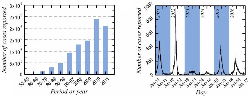
INTRODUCTION
According to a recent report of the world health organization (WHO), over 40% of the
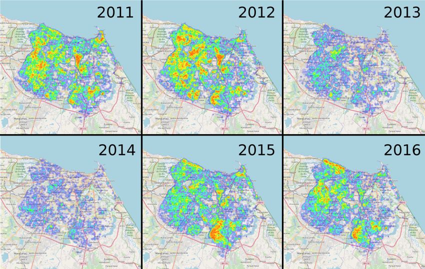
world’s population are at the risk of a dengue infection [1]. Alarmingly, in the last half-
century, a 20 to 30-fold increase of dengue cases has been monitored world-wide as shown
in Fig. 1 (left). Dengue fever is a vector-borne disease and thus requires a disease vector
to transmit the virus from one infected human to another susceptible one. Dengue virus
transmission occurs through bloodsucking female Aedes aegypti mosquitoes. Infected hu-
mans transmit the virus, up to maximally 12 days after first symptoms occur, to a mosquito
which further transmits the virus after an incubation period of 4-10 days [1]. Symptoms
include high fever, headache, vomiting, skin rash, and muscle and joint pains [2]. Aedes
aegypti is also responsible for the transmission of other severe vector-borne diseases such
as yellow fever, chikungunya and zika whose recent outbreaks are challenging health offi-
cials in different countries [3–5]. Vector-borne diseases are responsible for the death of more
than one million humans each year, disrupt health systems, and obstruct the development
of many countries [1]. As a consequence of the unavailability of vaccines and/or drug re-
sistance, as is the case for many vector-borne diseases, control measures such as personal
protection, reduction of vector breading habitats, and usage of insecticides are essential to
contain outbreaks [1, 6].
Recently, studies have demonstrated the poor correspondence between levels of infesta-
tion measured by entomological surveys at national and local level [8–10]. The correlation
between high infestation, measured by larval entomological indicators, and risk of dengue
epidemic has been shown to be weak in the most diverse scenarios [11–15]. Despite the
evidence of the low usefulness and incipient positive predictive value of these larval surveys
being extensively demonstrated, some countries still consider the thresholds of infestation
indices as a main indicative of epidemic risk and trigger of spatially-oriented vector control
actions [8, 9, 15].
In fact, there is pessimism about the ability of larval indicators to be good parameters
for the prediction of epidemics. Several authors have suggested the systematic use of pupal
indices and those that directly measure the density of the adult mosquito, even if this
implies a radical reformulation in the routines of vector control programs. They argue that
the larval indexes are no longer able to fulfill their main objective, which is, when estimated
2
Figure 1. Temporal evolution of the number of dengue cases. In the left panels, we show
the number of dengue cases that were reported to the WHO during the last half-century [1, 7].
Between 1995–2007, the shown numbers are averages over the indicated periods. The number of
cases has been increasing drastically during the last half-century. In the right panel, we show the
number of reported dengue cases per day in Fortaleza from 2011 to 2016.

the abundance of the adult vector, to anticipate the transmission of the disease [8, 10, 13,
15–17]. Moreover, pupal surveys and mosquito capture are of low cost-effectiveness and
inaccurate in low infestation scenarios where the mosquito has high survival due to optimal
climatic conditions and other factors, increasing vector competence and causing sustained
transmission of the virus with low pupal and mosquito densities.
   Urban mobility, as expressed by the movement of viremic humans, has become a more im-
portant factor than levels of infestation and abundance of the Aedes aegypti vector [18, 19].
Several studies point out the importance of the human movement in the spatio-temporal
dynamics of urban arboviruses transmitted by Aedes aegypti, in particular, dengue fever [20–
22]. In 2019, the Pan American Health Organization (PAHO) published a technical doc-
ument that points out that the risk stratification of transmission, using the most diverse
information available, is the path to better efficiency of vector control [23]. Theoretically,
mapping cities in micro-areas with different levels of transmission risk could make vector
control strategies more effective, especially in regions with limited human and financial
resources [24–26]. However, human mobility patterns are still not subject to accurate moni-
toring and can be crucial for the definition of high-risk spatial units that should be prioritized
by the national and local programs for the control of urban arboviruses transmitted by Aedes

                                               3
aegypti [8].
Predicting and containing dengue outbreaks is a demanding task due to the complex
nature of the underlying spreading process [27, 28]. Many factors such as environmental
conditions or the movements of humans within certain regions influence the spreading of
dengue [29–32]. The increasing danger of dengue infections makes it, however, necessary
to foster a better understanding of the spreading dynamics of dengue. In this work, we
study the spatio-temporal characteristics of dengue outbreaks in Fortaleza from 2011-2016
to characterize epidemic and non-epidemic years. Fortaleza, the capital of Ceará state is
one of the largest cities in Brazil and is located in the north-east of the country where
dengue and other neglected tropical diseases show a high prevalence [16, 33]. We show
in Fig. 1 (right) that up to 1000 dengue cases have been reported per day in Fortaleza
during 2011 and 2016. In our analysis, we identify regions that exhibit a large number of
dengue infections and mosquito larvae in different years, and also analyze the corresponding
correlations throughout all neighborhoods of Fortaleza. We observe that the correlation
length (i.e., the characteristic length scale of correlations between case numbers at different
locations in the system) is of the order of the system size. This provides strong support to
the fact that presence factors such as citizen mobility driving the spatial spreading of the
disease.
Motivated by the observation that people interact across long distances, we use a mean-
field model to compare the outbreak dynamics of two characteristic epidemic years with
corresponding analyses made for other regions [34]. In particular, we perform a Bayesian
Markov chain Monte Carlo parameter estimation for a mean-field susceptible-infected-
recovered (SIR) model which has been previously successfully applied to the modeling
of dengue outbreaks [34]. Our results provide insights into the spatio-temporal character-
istics of dengue outbreaks in densely populated areas and should therefore be relevant for
making dengue containment strategies more effective.
DATA SET
In total, we consider three data sets that are available as Supplemental Material. The first
data set consists of spatio-temporal information on dengue infections in the city of Fortaleza
from 2011 to 2016. These data have been provided by the Epidemiological Surveillance
4Year Number of cases reported
2011 33953
2012 38319
2013 8761
2014 5092
2015 26425
2016 21736
Table I. Number of dengue cases reported in Fortaleza between 2011 and 2016.
Division of Fortaleza Health Secretariat, and contains both the date when an infected per-
son reports a potential dengue infection to a physician and the corresponding geographic
location. Serology and clinical diagnosis were used to diagnose dengue infections. Dataset
that was provided by Fortaleza Health Secretariat has been anonymized. Epidemiological
and clinical variables have also been removed. We remove cases of infected tourists and
people who live in the metropolitan area of Fortaleza. The total number of dengue cases
between 2011 and 2016 in our data set after data processing is 133540. Table I shows the
number of cases reported for each year. Our second data set contains information about
Aedes aegypti larvae measurements in Fortaleza from 2011 to 2016. Measurement data is
available in fortnight intervals (i.e., every two weeks) from 113 strategic points (SP) (e.g.
junk yards) that are monitored by health authorities of Fortaleza over the whole city. A
SP is said to be positive if Aedes aegypti larvae have been found independent of the actual
amount. Data on Aedes aegypti infestation according to each Strategic Point are available
on the Fortaleza Daily Disease Monitoring System [35] and were tabulated and consolidated
by the epidemiological surveillance division team. Due to the influence of precipitation on
the mosquito population size [29], we also consider data from three different rain gauges in
Fortaleza during 2011 to 2016.
Dengue outbreaks in Fortaleza
According to the Brazilian ministry of health and the health administration of the prefec-
ture of Fortaleza, the population of Fortaleza had been at a high risk of a dengue infection
57000 12000
6000 Dengue cases Dengue cases
2011 10000 2012
Rainfall (×10) Rainfall (×10)
5000
Positive SP (×10) 8000 Positive SP (×10)
Measure
Measure
4000
6000
3000
4000
2000
1000 2000
0 0
0 4 8 12 16 20 24 0 4 8 12 16 20 24
Cycle Cycle
5000 3000
Dengue cases Dengue cases
4000 2013 2014
Rainfall (×10) Rainfall (×10)
Positive SP (×10) 2000 Positive SP (×10)
Measure
Measure
3000
2000
1000
1000
0 0
0 4 8 12 16 20 24 0 4 8 12 16 20 24
Cycle Cycle
6000 4000
Dengue cases Dengue cases
5000 2015 2016
Rainfall (×10) 3000 Rainfall (×10)
4000 Positive SP (×10)
Measure
Measure
3000 2000
2000
1000
1000
0 0
0 4 8 12 16 20 24 0 4 8 12 16 20 24
Cycle Cycle
Figure 2. The number of reported dengue cases, positive SPs and rainfall as a function
of time from 2011 to 2016. For each year from 2011 until 2016, we show the number of reported
dengue cases, positive SPs and the rainfall as a function of time. One time interval (cycle) is one
fortnight. The number of positive SPs and amount of rain in liters per square meter have been
rescaled by a factor of 10. There is no larvae measurement data available for 2016.
during the years 2011, 2012, 2015, and 2016 that are classified as epidemic years [36]. The
number of reported dengue cases in this time period is given in Table I and shown in Fig. 1
(right). Considering the population size of 2.5 million [37], an alarmingly high number of
several hundred up to almost 1000 new infections per day have been reported during this
time period. As shown in Fig. 2, the number of reported dengue cases starts to increase
6Year
Correlations
2011 2012 2013 2014 2015 2016
τmax (D, R) 5 3 2 2 2 0
τmax (D, SP) 2 2 1 3 3 -
τmax (SP, R) 2 1 -1 -1 -1 -
Table II. The maximum correlation coefficient time lags from 2011 until 2016. For
each year from 2011 until 2016, we compute the correlation coefficients of the number of reported
dengue cases (D), positive SPs and the rainfall (R) for different time lags τ . The value of τ = 1
corresponds to one fortnight. We show the time lags that correspond to a maximum correlation
coefficient. There is no SP data available for 2016.
in January and February just shortly after the beginning of the rain season and typically
reaches its peak before July. This shows that the corresponding climate conditions facilitate
the growth of mosquito populations. In addition, we also show the time evolution of the
number of positive SPs (i.e., the number of strategic measurement points where Aedes
aegypti larvae have been found). The data in Fig. 2 indicates that the number of positive
SPs changes according to the rainfall, because the curves behave very similar although their
relative amplitudes vary substantially from year to year.
To better understand the correlations between rainfall, larvae growth, and dengue cases
we compute the corresponding correlation coefficients for different time lags τ . A time lag
of τ = 1 means that the two considered curves are shifted by one fortnight. In Table II,
we show the time lags τmax that correspond to the maximum correlation coefficient. In
the case of dengue occurrences and rainfall, we find a mean value of τ̄max (D, R) = 2.3(2)
fortnights. This result agrees with the well with findings of other studies [29] reporting
that a maximum of dengue cases will be observed a few weeks up to a few months after
the rainfall maximum. The maximum correlation between dengue cases and SPs indicates
that the dengue incidence reaches a maximum after τ̄max (D, SP ) = 2.2(8) fortnights after
a maximum of positive SPs has been found. This result implies that the number of positive
SPs may be an appropriate early warning sign to estimate when the number of dengue cases
reaches its maximum. Despite the very similar curve shapes, the results are less conclusive
in the case of correlations between rainfall and positive SPs. In some years, the maximum
7Figure 3. Dengue outbreaks in Fortaleza from 2011 until 2016. Heat maps of all dengue
cases in Fortaleza from 2011 until 2016. Blue areas correspond to regions with a low prevalence
of dengue cases whereas red ones indicate large dengue outbreaks. The epidemic years are 2011,
2012, 2015 and 2016. All heat maps have been generated with Folium [38].
number of positive SPs is found after the rainfall maximum, whereas the opposite situation
occurs in other years, which means that they are uncorrelated. This can be also seen by
comparing the time evolutions of rainfall and the number of positive SPs in Fig. 2. A
possible reason to explain this result may be the fact that a SP was considered as positive
even if a small amount of larvae was found at this location. For this reason the positiveness
of a SP indicates the spatial extent of mosquitoes and not their concentration. Therefore,
correlations between rainfall and positive SPs have to be interpreted with caution. Still,
the very similar shapes of the positive SP and the rainfall curves indicate that the spatial
spread of the mosquito changes with the amount of rain. The influence of climate conditions
on dengue outbreaks in Brazil has also been recently analyzed in reference [29]. Due to
the equatorial location of Fortaleza, the mean temperature over one year is 26.3 ± 0.6◦ C
and can be regarded as constant with only limited impact on the local dengue spreading
8Figure 4. Positive SPs in Fortaleza from 2011 until 2015. Heat maps of the larvae measure-
ment outcomes in Fortaleza from 2011 until 2015. Each district has a different number of SPs. If
larvae are found, the SP measurement is said to be positive. Blue areas correspond to regions with
a low number of positive SPs, whereas red ones indicate the opposite. All heat maps have been
generated with Folium [38].
dynamics [39].
In addition to the temporal information on dengue cases in Fortaleza, we collected data
about the geographical locations of all infection cases. We illustrate the geographical dis-
tribution of dengue cases in Fig. 3 from 2011 until 2016. If the total number of dengue
infections in a certain area is large over the course of one year, this area appears in red.
Areas with small numbers of dengue infections are colored blue. In 2011 and 2012 the main
outbreaks occur in similar regions and cover almost the whole city except some parts in the
eastern outskirts. In the non-epidemic years 2013 and 2014, the overall dengue prevalence is
clearly reduced. However, some parts in the city center in the north west that also exhibit
large numbers of dengue cases in the epidemic years are still at a high risk of dengue out-
breaks. Also in the epidemic years 2015 and 2016, some neighborhoods in the south show a
9high dengue prevalence.
In addition to the geographical location of dengue cases, we also show a heat map of the
spatial distribution of positive SPs in Fig. 4. Interestingly, and in contrast to the spatial
distribution of dengue cases, the majority of positive SPs are located at the same place in
Fortaleza regardless of the year. In particular the city center and some parts in the north
and south west of the town exhibit a large number of positive SPs. While according to
Fig. 4 the regions of major outbreaks change substantially between 2011, 2013 and 2015,
the number of positive SPs does not at all. Concerning the outbreak years 2015 and 2016,
the recurrent dengue outbreaks and numbers of positive SPs seem to be even anti-correlated.
These observations suggest that an effective disease intervention measure should target the
neighborhoods which exhibit recurrent dengue outbreaks instead of numbers of positive SPs.
In particular, the density of SPs is not homogeneous, which could be another reason why
they fail to reproduce the major outbreaks of 2015 and 2016 in the south east of the city.
SPATIO-TEMPORAL CORRELATIONS
For a better understanding of the spreading dynamics of dengue in urban environments,
it is crucial to analyze the influence of local dengue outbreaks on outbreaks at other locations
and vice-versa. In this way, We therefore now focus on spatio-temporal correlations between
dengue incidences of different districts. In total, there are 118 neighborhoods in Fortaleza,
and for each neighborhood i we consider the number of reported dengue cases NCti at time t
and the corresponding population POPi . The disease prevalence in neighborhood i at time
t is given by
NCti
pti = . (1)
POPi
We characterize the spatio-temporal correlations of dengue outbreaks between sites i and j
by
PT
pt−τ
t
1 t=1 i − hp i i p j − hp j i
cij (τ, rij ) = , (2)
T σ1 σ2
where τ denotes a time lag, rij is the distance between neighborhood i and neighborhood
2
j, and σi2 = T −1 Tt=1 (pti − hpi i) represents the variance. In our following analysis, we
P
consider two time intervals: (i) four weeks (i.e., T = 12) and (ii) two weeks (i.e., T = 26).
Dengue outbreaks that occur in a certain region of the city may lead to outbreaks in
101.0 6
2011 2011
0.8 5
2012 2012
2013 4 2013
hci j (τ0 )i
0.6
P(ci j )
2014 3 2014
0.4 2015 2015
2
2016 2016
0.2 1
0.0 0
0 5 10 15 20 25 30 −1.0 −0.5 0.0 0.5 1.0
ri j ci j (τ0 )
0.8 3
2011 2011
0.6 2012 2012
2013 2 2013
hci j (τ1 )i
P(ci j )
0.4 2014 2014
2015 2015
1
2016 2016
0.2
0.0 0
0 5 10 15 20 25 30 −1.0 −0.5 0.0 0.5 1.0
ri j ci j (τ1 )
0.6 3
2011 2011
2012 2012
0.4 2013 2 2013
hci j (τ2 )i
P(ci j )
2014 2014
2015 2015
0.2 1
2016 2016
0.0 0
0 5 10 15 20 25 30 −1.0 −0.5 0.0 0.5 1.0
ri j ci j (τ2 )
Figure 5. Correlations for different time lags, distances and years and their corre-
sponding distributions. The left panels show average of the correlation coefficients hcij (τ )i as
a function of the distance rij between neighborhoods i and j time lags of τ0 = 0 weeks, τ1 = 2
weeks and τ2 = 4 weeks. As depicted, epidemic years (2011, 2012, 2015, and 2016) present a higher
value of hcij (τ )i when compared to non-epidemic years (2013 and 2014). The right panels show the
corresponding distribution P (cij ) of the correlation coefficients cij (τ, rij ). Epidemic years present
a negative skewness for P (cij ), while non-epidemic years have no skewness.
another more distant region due to human mobility, because mosquitoes at the new location
then have the possibility of getting in contact with the virus [30–32]. To analyze this effect
and identify characteristic correlation length-scales, we study the correlation between the
11dengue prevalence in neighborhood i and another neighborhood j located within a distance
of rij . Here, the distance rij is the distance between the barycenters of neighborhoods i and
j extracted from their geographical contours. Specifically, we study the correlations between
neighborhoods i and j, i.e. cij (τ, rij ) as defined by Eq. (2), for different time lags τ and radii
rij . According to the definition of cij (τ, rij ) in Eq. (2), a correlation length ξ smaller than
our considered system size would lead to an observable decay of cij (τ, rij ) for rij > ξ. In all
considered years, the correlations cij (τ ) only vary slightly with the distance rij , as shown
in Fig. 5. Within the error bars of our data we do not observe a substantial decay of cij (τ )
for values of rij smaller than the system size of about 15 km. We thus conclude that the
characteristic correlation length ξ is of the order of the system size.
We choose three time lags, namely, τ0 = 0 weeks, τ1 = 2 weeks and τ2 = 4 weeks
which are of the order of the transmission time scale of 12 days [1]. The dependence of the
correlations on different time lags, distances and years is shown in Fig. 5 (left). For no time
lag, τ0 = 0 weeks, or a time lag of τ1 = 2 weeks, we find that the correlations are substantially
larger in the epidemic years 2011, 2012, 2015 and 2016 as compared to the non-epidemic
years 2013 and 2014. However, in 2016 the correlations are less pronounced compared to
other epidemic years since the outbreaks are widely distributed and their densities rather
small, as shown in Fig. 3. In the case of the larger time lag, τ2 = 4 weeks, the average
correlation hcij (τ2 )i for epidemic years decreases when compared with smaller time lags.
This behavior is in accordance with observation, since a time lag of 4 weeks exceeds the
dengue transmission period, and we expect to find smaller correlations. In Fig. 5 (right), we
show the corresponding distributions of P (cij ) and find that they allow to clearly distinguish
between epidemic and non-epidemic years for no time lag and a time lag τ1 = 2 weeks. In
particular in the case of no time lag, the correlations are substantially larger in epidemic
years compared to the non-epidemic ones.
It is unlikely that disease vectors are responsible for such correlation effects over distances
of multiple kilometers due to their limited movement capabilities. In particular, it is known
that the maximum flight distance reached by the Aedes aegypti from its breeding location
is of the order of approximately 100 meters. On the other hand, humans travel through the
densely populated urban region on a daily basis, and may transfer the virus to Aedes aegypti
mosquitoes at different locations. This virus transfer mechanism is therefore compatible with
the large correlation lengths revealed in this study and also agrees well with recent studies
12that suggest that human mobility is a key component of dengue spreading [30–32].
ESTIMATING DISEASE TRANSMISSION PARAMETERS
As mentioned in the previous section, the considered dengue outbreaks in Fortaleza ex-
hibit a correlation length ξ which is of the order of the underlying system size. Based on
this observation, we apply mean-field epidemic model, as a first approximation, to further
characterize the observed spreading dynamics. In particular, we aim at comparing the dis-
ease transmission parameters of dengue outbreaks in Fortaleza with the results of previous
studies [34]. To do so, we consider the two epidemic years 2012 and 2015 and perform a
Bayesian Markov chain Monte Carlo parameter estimation for a SIR model that has been
previously applied in the context of dengue outbreaks in Thailand [34]. More details about
the methodology are presented in Appendix A. Such a parameter estimation enables us to
determine the basic reproduction number R0 of dengue outbreaks in Fortaleza and compare
it with the values of other disease outbreaks. The basic reproduction number constitutes an
important epidemiological measure and is defined as the average number of secondary cases
originating from one infectious individual during the initial outbreak period (i.e., in a fully
susceptible population) [40]. Different models exist to characterize and predict epidemic
outbreaks [40–44].
In the case of dengue, some models explicitly incorporate a mosquito population, whereas
others take into account such effects by using an effective spreading rate [34, 45]. According
to Ref. [34], an explicit treatment of vector populations just increases the number of modeling
parameters and may not lead to a better agreement between model and data. We therefore
do not explicitly model a vector population and consider a SIR model with an effective
spreading rate which has been found to capture essential features of dengue outbreaks in
Thailand [34]. The governing equations are
dS I
= µH N − β S − µH S, (3)
dt N
dI I
= β S − γH I − µH I, (4)
dt N
dR
= γH I − µH R, (5)
dt
where N = S + I + R is the human population size and S = S(t), I = I(t), R = R(t)
the numbers of susceptible, infected and recovered individuals at time t, respectively. The
13human mortality rate is denoted by µH and the human recovery rate by γH . The term µH N
in Eq. (3) corresponds to the birth rate and is chosen such that the population size is kept
constant. Furthermore, the composite human-to-human transmission rate β accounts for
transitions from susceptible to infected. The relation
mc2 βH βV
β≈ (6)
µV
connects β with the mosquito-to-human transmission rate per bite βH , human-to-mosquito
transmission rate βV , number of mosquitoes per person m, mean rate of bites per mosquito
c, and mosquito mortality rate µV [34]. The basic reproduction number of the SIR model
is [40]
β
R0 = . (7)
µH + γH
For R0 > 1 there exists a stable endemic state whereas the disease-free equilibrium is stable
for R0 ≤ 1. In addition to Eqs. (3)-(5), we define the time evolution of the cumulative
number of reported dengue cases C = C(t) by
dC I
= pβ S, (8)
dt N
where p is the fraction of infected individuals that were diagnosed with dengue and reported
to the health officials. We set the population size to N = 2.4 million in agreement with the
most recent census data of Fortaleza [37]. Moreover, we use a mortality rate of µH = 1/76 y−1
in accordance with the latest World Bank life expectancy estimates [46].
A parameter estimation based on Eqs. (3)-(5) and (8) means that we have to determine
the parameters β, γH , p and the initial fraction of recovered individuals r0 = R(0)/N that
best describe the observed dengue outbreaks. More specifically, we use Bayes’ theorem to
determine the posterior parameter distribution
P (θ|D) ∝ P (D|θ) P (θ) (9)
based on the likelihood function P (D|θ) (i.e., the conditional probability of obtaining the
data D for given model parameters θ) and the prior parameter distribution P (θ). The
actual Bayesian Markov chain Monte Carlo algorithm is described in Appendix A.
In order to be able to compare our results with the ones of Ref. [34] and to obtain a
full infection period, we consider November as our starting month, because the rainfall then
typically reaches a minimum. In Table III, we summarize the inferred model parameters,
14median values, and 95% confidence intervals of the posterior distributions. In addition,
we also present the maximum likelihood (ML) estimates which we use to compare the SIR
model with the actual dengue case data in Fig. 7. We find good agreement between the model
prediction and the actually reported number of dengue cases. Only the dengue outbreak
peak between April and June 2012 is difficult to capture because due to overwhelming
number of up to 1000 new infections per day.
35 90
30 2012 80 2012
70
25 2015 2015
60
20 50
PDF
PDF
15 40
30
10
20
5 10
0 0
0.12 0.14 0.16 0.18 0.20 0.22 0.24 0.10 0.12 0.14 0.16 0.18 0.20
β γH
160 9
140 2012 8 2012
120 7
2015 2015
6
100
5
PDF
PDF
80
4
60
3
40 2
20 1
0 0
0.02 0.03 0.04 0.05 0.06 0.07 0.08 0.00 0.05 0.10 0.15 0.20 0.25 0.30 0.35
p r0
Figure 6. Posterior distributions of SIR model parameters. The probability density func-
tions (PDFs) of the posterior distributions of the modified SIR model as defined by Eqs. (3)-(5)
and (8). The two epidemic years 2012 (orange bars) and 2015 (blue bars) have been considered for
the parameter estimation.
After estimating the SIR model parameters for the epidemic years 2012 and 2015, we
now compare the obtained estimates with the ones of Ref. [34] which focuses on dengue
outbreaks in Thailand. In ref [34], the number of reported dengue hemorrhagic fever (DHF)
cases, a more severe form of dengue fever, has been used, while we considered the number
of all reported dengue cases. The total number of mentioned DHF cases in Thailand is
roughly 70000 with a total population size of 46.8 million in 1984 [34]. In contrast to these
results, the number of reported dengue cases in Fortaleza in 2012 is almost 40000 with a
15Parameter ML Median 95% CI
β d−1
0.1453 (2012) 0.1648 (2012) (0.1409, 0.2138) (2012)
Composite transmission rate 0.1518 (2015) 0.1606 (2015) (0.1453, 0.1966) (2015)
γH d−1
0.1011 (2012) 0.1121 (2012) (0.1005, 0.1650) (2012)
Human recovery rate 0.1009 (2015) 0.1064 (2015) (0.1004, 0.1299) (2015)
p 0.0368 (2012) 0.0432 (2012) (0.0348, 0.0609) (2012)
Probability of reporting a dengue case 0.0218 (2015) 0.0234 (2015) (0.0206, 0.0291) (2015)
r0 0.0594 (2012) 0.0769 (2012) (0.0066, 0.2928) (2012)
Initial fraction of humans recovered 0.0618 (2015) 0.0636 (2015) (0.0045, 0.2609) (2015)
R0 1.4367 (2012) 1.5384 (2012) (1.2184, 1.9584) (2012)
Basic reproduction number 1.5039 (2015) 1.4904 (2015) (1.3471, 1.7396) (2015)
Table III. Posterior parameter estimations. Based on given prior SIR parameter distributions,
the corresponding posterior distributions for the dengue outbreaks in 2012 and 2015 have been ob-
tained using Bayesian Markov chain Monte Carlo sampling. For both years an additional maximum
likelihood (ML) parameter estimate is given. The posterior distributions are characterized by their
median values and their 95% confidence intervals (CI).
total population size of 2.5 million. This alarming difference may be partially a result of
the different definitions of reported cases (DHF versus dengue fever) as well as due to sub-
notification, but it also points out to the need of better control measures to contain the
outbreaks in Fortaleza. Overall, the parameter estimation for the epidemic years 2012 and
2015 leads to values in a similar range compared to the results of Ref. [34]. The ML estimates
of p and r0 are a factor 2-3 larger in our parameter estimation. On the other hand, the ML
estimates of β and γ are slightly smaller in Fortaleza. The basic reproduction number as
defined in Eq. (7) (basically the fraction of β and γH ) is 1.44 (2012) and 1.50 (2015) and
thus exhibits a value within the confidence interval of Ref. [34]. This result suggests that
the dengue outbreaks in both locations show similar characteristics. In other words, the
average number of secondary dengue cases originating from one infection is almost identical
in both locations.
1640 30
cases reported (thousands)
cases reported (thousands)
Cumulative number of
Cumulative number of
35
25
30
20
25
SIR SIR
20 15
15
Data Data
10
10
5
5
0 0
0 50 100 150 200 250 300 350 400 0 50 100 150 200 250 300 350 400
Days (November 2011-December 2012) Days (November 2014-December 2015)
Figure 7. SIR model fit for the epidemic years 2012 and 2015. The maximum likelihood
fits of the SIR model (black solid lines) as defined by Eqs. (3)-(5) and (8) for the epidemic years
2012 (left) and 2015 (right). The cumulative number of reported dengue cases according to our
data set is indicated by green circles.
DISCUSSION
The re-emergence of dengue and other neglected tropical diseases is a major threat in
many countries. We analyzed the recent dengue outbreaks in Fortaleza as one of the largest
Brazilian cities. We identified regions which exhibit a large number of dengue infections and
Aedes aegypti larvae over different years. Our results show that the characteristic length
scale of correlation effects between the number of cases at different locations is of the order
of the system size. One possible explanation for this observation is that the human mobility,
and not the epidemic vector (the mosquito), is the major mechanism responsible for the
dissemination of the virus. Human movement seems to be a crucial factor in the transmission
dynamics, particularly in large tropical cities where successive dengue epidemics have been
recorded, suggesting that the mosquito is highly adapted, with low intra-urban infestation
differentials. In addition, we also compared the disease transmission characteristics of dengue
outbreaks in Fortaleza with the ones in Thailand. Our comparison showed that the number
of dengue cases in Fortaleza is much higher compared to the outbreak data of Ref. [34]. We
also found that the obtained basic reproduction number of dengue outbreaks in Fortaleza
is within the confidence interval of the value mentioned in Ref. [34]. This means that the
average number of secondary dengue cases originating from one infection is almost identical
in both locations. Moreover, we classified epidemic and non-epidemic years based on an
analysis of spatio-temporal correlations and their corresponding distributions. Finally, we
17found that the spatial-temporal correlations are of the size of the system likely due to human
mobility.
Appendix A: Bayesian Markov chain Monte Carlo
To compute the parameter distributions of the SIR model defined by Eqs. (3)-(5) and
(8), we have to determine the probability distribution P (θ|D) of θ = (β, γH , p, r0 ) given our
data on the cumulative number of reported dengue cases D. According to Bayes’ theorem,
we express the posterior distribution
P (θ|D) ∝ P (D|θ) P (θ) , (A1)
in terms of the likelihood function P (D|θ) and the prior parameter distribution P (θ). We
assume that the likelihood function P (D|θ) is a Gaussian distribution of the error E with
zero mean and variance σ 2 , i.e.,
E2
P (D|θ) ∝ exp − 2 . (A2)
2σ
To compute the error, we discretize the infection period in monthly time intervals described
by the times ti with i ∈ {1, 2, . . . , 12} and evaluate yi (θ) = C(ti )/N for a given θ. In the
next step, we compare the prediction of our model yi (θ) with the actual cumulative number
of reported dengue cases Di at time ti and use the least square error
12
X
2
E = [Di − yi (θ)]2 (A3)
i=1
as our error estimate in Eq. (A2) [34]. For a given prior parameter distribution P (θ),
we compute the posterior distribution P (D|θ) using Bayesian Markov chain Monte Carlo
sampling with a Metropolis update scheme [34, 47]. After initializing the parameter vector
with θ0 drawn from the prior distribution P (θ), the nth iteration of the algorithm is defined
as follows:
1. A new parameter set θ∗ is drawn from the proposal distribution J (θ∗ |θn ).
2. The acceptance probability for θ∗ is computed according to (Metropolis algorithm)
P (θ∗ |D) P (D|θ∗ ) P (θ∗ )
r = min , 1 = min ,1 . (A4)
P (θn |D) P (D|θn ) P (θn )
183. Draw a random number ∼ U (0, 1) and set
θ∗ if < r,
n+1
θ = (A5)
θn otherwise.
This update procedure implies that a new parameter set is always accepted if the new
likelihood function value is greater or equal than the one of the previous iteration, i.e., if
P (D|θ∗ ) ≥ P (D|θn ). For the described Metropolis algorithm, the proposal distribution
J (θ∗ |θn ) must be symmetric. According to Ref. [47], a multivariate Gaussian distribution
J (θ∗ |θn ) ∼ N θn |λ2 Σ
(A6)
may be used as proposal distribution. The covariance matrix is denoted by Σ and the
corresponding scaling factor by λ. Every 500 iterations, the covariance matrix and the
scaling factor are updated using the following update procedure [34, 47]:
Σk+1 = pΣk + (1 − p)Σ∗ ,
∗
α − α̂
(A7)
λk+1 = λk exp ,
k
where Σ∗ and α∗ are the covariance matrix and the acceptance rate of the last 500 iterations,
√
respectively. Furthermore, p = 0.25 and the initially Σ0 = I and λ0 = 2.4/ d where I is
the d × d identity matrix and d the number of estimated parameters. The target acceptance
rate is [47]
0.44 if d = 1,
α̂ = (A8)
0.23 otherwise.
For evaluating Eq. (A4), we have to compute the least-square error for the new proposed
parameter set θ∗ according to Eq. (A3) to then obtain the likelihood function value P (D|θ∗ )
based on Eq. (A2). To obtain good convergence behavior, we set the variance of our like-
lihood distribution to σ 2 = 1/20. Convergence is measured in terms of the Gelman-Rubin
test [47]. Therefore, we consider four independent Markov chains. Every chain is initial-
ized with a different random parameter set which is drawn from the corresponding uniform
distributions. The posterior parameter distribution is considered to be converged if the vari-
ance between the chains is similar to the variance within the chain (Gelman-Rubin test).
19101 100
100 chain 1 10−1 chain 1
10−1 chain 2 10−2 chain 2
10−2 chain 3 10−3 chain 3
Error
Error
10−3 chain 4 10−4 chain 4
10−4 10−5
10−5 10−6
10−6 10−7
100 101 102 103 104 105 106 100 101 102 103 104 105 106
Iterations Iterations
Figure A.1. Convergence of Bayesian Markov chain Monte Carlo parameter estima-
tion. For both epidemic years 2012 (left) and 2015 (right), four different chains with different
initial conditions have been considered to perform Bayesian Markov chain Monte Carlo parameter
estimation. The algorithm is considered to be converged to the posterior distribution if the variance
between the chains is similar to the variance within the chains (Gelman-Rubin test) [47].
In Fig. A.1, we illustrate the convergence behavior. After reaching convergence, we pro-
duce 105 more samples without updating the covariance matrix and construct the posterior
parameter distribution based on every 5th sample.
For both epidemic years, we use four independent Markov chains with different initial
parameter sets θ = (β, γH , p, r0 ) that are drawn from uniform posterior distributions. If
the variance between the chains is similar to the variance within the chain (Gelman-Rubin
test), we consider the posterior distribution to be converged. Every new proposed set of
parameters θ∗ is accepted with probability (Metropolis algorithm) [47]
P (θ∗ |D) P (D|θ∗ ) P (θ∗ )
r = min , 1 = min ,1 . (A9)
P (θ|D) P (D|θ) P (θ)
The resulting posterior distributions are shown in Fig. 6. We find similar posterior distri-
butions of the parameters β, γH and r0 for both epidemic years. The distributions of p
(fraction of infected individuals that were diagnosed with dengue and reported to the health
officials) are different due to the larger number of reported dengue cases in 2012 (38197)
compared to 2015 (26176).
Declarations
20Availability of data and material
All data generated or analysed during this study are included in this published article
[and its supplementary information files].
Competing interests
The authors declare no competing interest.
Acknowledgements
We acknowledge financial support from the Brazilian agencies CNPq, CAPES, the FUN-
CAP Cientista Chefe program, and from the National Institute of Science and Technology
for Complex Systems (INCT-SC) in Brazil. LB acknowledges financial support from the
SNF Early Postdoc. Mobility fellowship on “Multispecies interacting stochastic systems in
biology” and the Army Research Office (W911NF-18-1-0345).
Authors’ contributions
All authors designed research. GSS and ASLN collected and prepared the Dengue data
sets. SDRS, LB, and JPdCN processed the Dengue data. All authors analyzed and inter-
preted the Dengue data. SDSR, LB, ASLN, HH and JSA wrote the manuscript. All authors
read and approved the final manuscript.
[1] World Health Organization. Sustaining the drive to overcome the global impact of neglected
tropical diseases; 2013.
[2] World Health Organization. Dengue: guidelines for diagnosis, treatment, prevention and
control; 2009.
[3] Barret ADT, Higgs S. Yellow Fever: A Disease that Has Yet to be Conquered. Annu Rev
Entomol. 2007;(52):209–229.
21[4] Charrel RN, et al. Chikungunya outbreaks-the globalization of vectorborne diseases. N Engl
J Med. 2007;(356):769.
[5] Brasil P, et al. Zika Virus Infection in Pregnant Women in Rio de Janeiro. N Engl J Med.
2016;(375):2321–2334.
[6] Hotez PJ, Bottazzi ME, Franco-Paredes C, Ault SK, Periago MR. The Neglected Tropical
Diseases of Latin America and the Caribbean: A Review of Disease Burden and Distribution
and a Roadmap for Control and Elimination. PLoS Negl Trop Dis. 2008;(2):e300.
[7] World Health Organization. A global brief on vector-borne diseases; 2014.
[8] Enslen AW, Lima Neto AS, Castro MC. Infestation measured by Aedes aegypti larval surveys
as an indication of future dengue epidemics: an evaluation for Brazil. Transactions of The
Royal Society of Tropical Medicine and Hygiene. 2020;.
[9] MacCormack-Gelles B, Neto ASL, Sousa GS, do Nascimento OJ, Castro MC. Evaluation of
the usefulness of Aedes aegypti rapid larval surveys to anticipate seasonal dengue transmission
between 2012–2015 in Fortaleza, Brazil. Acta Tropica. 2020;205:105391.
[10] Sanchez L, Vanlerberghe V, Alfonso L, del Carmen Marquetti M, Guzman MG, Bisset J,
et al. Aedes aegypti larval indices and risk for dengue epidemics. Emerging infectious diseases.
2006;12(5):800.
[11] Cromwell EA, Stoddard ST, Barker CM, Van Rie A, Messer WB, Meshnick SR, et al. The
relationship between entomological indicators of Aedes aegypti abundance and dengue virus
infection. PLoS neglected tropical diseases. 2017;11(3).
[12] Focks DA, Chadee DD. Pupal survey: an epidemiologically significant surveillance method
for Aedes aegypti: an example using data from Trinidad. The American journal of tropical
medicine and hygiene. 1997;56(2):159–167.
[13] Focks DA, et al. A review of entomological sampling methods and indicators for dengue
vectors. World Health Organization; 2004.
[14] Gubler DJ. Dengue and dengue hemorrhagic fever. Clinical microbiology reviews.
1998;11(3):480–496.
[15] Bowman LR, Runge-Ranzinger S, McCall P. Assessing the relationship between vector in-
dices and dengue transmission: a systematic review of the evidence. PLoS neglected tropical
diseases. 2014;8(5).
[16] MacCormack-Gelles B, Neto ASL, Sousa GS, Nascimento OJ, Machado MM, Wilson ME,
22et al. Epidemiological characteristics and determinants of dengue transmission during epidemic
and non-epidemic years in Fortaleza, Brazil: 2011-2015. PLoS neglected tropical diseases.
2018;12(12):e0006990.
[17] Tun-Lin W, Kay B, Barnes A, Forsyth S. Critical examination of Aedes aegypti indices:
correlations with abundance. The American journal of tropical medicine and hygiene.
1996;54(5):543–547.
[18] Bouzid M, Brainard J, Hooper L, Hunter PR. Public health interventions for Aedes control
in the time of Zikavirus–a meta-review on effectiveness of vector control strategies. PLoS
neglected tropical diseases. 2016;10(12).
[19] Stoddard ST, Forshey BM, Morrison AC, Paz-Soldan VA, Vazquez-Prokopec GM, Astete H,
et al. House-to-house human movement drives dengue virus transmission. Proceedings of the
National Academy of Sciences. 2013;110(3):994–999.
[20] Vazquez-Prokopec GM, Bisanzio D, Stoddard ST, Paz-Soldan V, Morrison AC, Elder JP, et al.
Using GPS technology to quantify human mobility, dynamic contacts and infectious disease
dynamics in a resource-poor urban environment. PloS one. 2013;8(4).
[21] Vazquez-Prokopec GM, Kitron U, Montgomery B, Horne P, Ritchie SA. Quantifying the
spatial dimension of dengue virus epidemic spread within a tropical urban environment. PLoS
neglected tropical diseases. 2010;4(12).
[22] Vazquez-Prokopec GM, Stoddard ST, Paz-Soldan V, Morrison AC, Elder JP, Kochel TJ,
et al. Usefulness of commercially available GPS data-loggers for tracking human movement
and exposure to dengue virus. International journal of health geographics. 2009;8(1):68.
[23] Organization PAH. Technical document for the implementation of interventions based on
generic operational scenarios for Aedes aegypti control. PAHO Washington, DC; 2019.
[24] Organization WH, et al. Handbook for integrated vector management. World Health Orga-
nization; 2012.
[25] Quintero J, Brochero H, Manrique-Saide P, Barrera-Pérez M, Basso C, Romero S, et al.
Ecological, biological and social dimensions of dengue vector breeding in five urban settings
of Latin America: a multi-country study. BMC infectious diseases. 2014;14(1):38.
[26] Caprara A, Lima JWdO, Marinho ACP, Calvasina PG, Landim LP, Sommerfeld J. Irregular
water supply, household usage and dengue: a bio-social study in the Brazilian Northeast.
Cadernos de saude publica. 2009;25:S125–S136.
23[27] Guzzetta G, Marques-Toledo CA, Rosà R, Teixeira M, Merler S. Quantifying the spatial spread
of dengue in a non-endemic Brazilian metropolis via transmission chain reconstruction. Nat
Commun. 2018;9(1):2837.
[28] Antonio FJ, Itami AS, de Picoli S, Teixeira JJV, dos Santos Mendes R. Spatial patterns of
dengue cases in Brazil. PloS one. 2017;12(7):e0180715.
[29] Stolerman L, Maia P, Kutz JN. Data-Driven Forecast of Dengue Outbreaks in Brazil: A
Critical Assessment of Climate Conditions for Different Capitals. arXiv:170100166. 2016;.
[30] Stoddard ST, et al. House-to-house human movement drives dengue virus transmission. Proc
Natl Acad Sci. 2013;(110):994–999.
[31] Jr RCR, Stoddard ST, Scott TW. Socially structured human movement shapes dengue trans-
mission despite the diffusive effect of mosquito dispersal. Epidemics. 2014;(6):30–36.
[32] Chris M Stone DMF Samantha R Schwab, Fefferman NH. Human movement, cooper-
ation and the effectiveness of coordinated vector control strategies. J R Soc Interface.
2017;(14):20170336.
[33] Lindoso JAL, Lindoso AABP. Neglected tropical diseases in Brazil. Rev Inst Med trop S
Paulo. 2009;(51):247–253.
[34] Pandey A, Mubayi A, Medlock J. Comparing vector–host and SIR models for dengue trans-
mission. Math Biosci. 2013;246(2):252–259.
[35] Fortaleza Daily Disease Monitoring System (SIMDA). https://pt.climate-data.org/america-
do-sul/brasil/ceara/fortaleza-2031/, retrieved June 3, 2020;.
[36] Ministério da Saúde do Brasil. Diretrizes nacionais para prevenção e controle de epidemias de
dengue. 2009;.
[37] https://cidades.ibge.gov.br/brasil/ce/fortaleza/panorama, retrieved December 9, 2018;.
[38] https://python-visualization.github.io/folium/, retrieved May 4, 2020;.
[39] https://pt.climate-data.org/america-do-sul/brasil/ceara/fortaleza-2031/, retrieved December
9, 2018;.
[40] Keeling MJ, Rohani P. Modeling Infectious Diseases in Humans and Animals. Princeton
University Press; 2008.
[41] Böttcher L, Woolley-Meza O, Araújo NAM, Herrmann HJ, Helbing D. Disease-induced re-
source constraints can trigger explosive epidemics. Sci Rep. 2015;5:16571.
[42] Böttcher L, Woolley-Meza O, Goles E, Helbing D, Herrmann HJ. Connectivity disruption
24sparks explosive epidemic spreading. Phys Rev E. 2016;93(4):042315.
[43] Böttcher L, Nagler J, Herrmann HJ. Critical Behaviors in Contagion Dynamics. Phys Rev
Lett. 2017;118:088301.
[44] Böttcher L, Andrade J, Herrmann HJ. Targeted Recovery as an Effective Strategy against
Epidemic Spreading. Sci Rep. 2017;7(1):14356.
[45] Fitzgibbon W, Morgan J, Webb G. An outbreak vector-host epidemic model with spatial struc-
ture: the 2015–2016 Zika outbreak in Rio De Janeiro. Theor Biol Med Model. 2017;14(1):7.
[46] https://data.worldbank.org/indicator/SP.DYN.LE00.IN, retrieved December 9, 2018;.
[47] Gelman A, Stern HS, Carlin JB, Dunson DB, Vehtari A, Rubin DB. Bayesian data analysis.
Chapman and Hall/CRC; 2013.
25You can also read