Supercooled liquid water and secondary ice production in Kelvin-Helmholtz instability as revealed by radar Doppler spectra observations
←
→
Page content transcription
If your browser does not render page correctly, please read the page content below
Atmos. Chem. Phys., 21, 13593–13608, 2021
https://doi.org/10.5194/acp-21-13593-2021
© Author(s) 2021. This work is distributed under
the Creative Commons Attribution 4.0 License.

Supercooled liquid water and secondary ice production in
Kelvin–Helmholtz instability as revealed by radar Doppler
spectra observations
Haoran Li1,2 , Alexei Korolev3 , and Dmitri Moisseev2,4
1 StateKey Laboratory of Severe Weather, Chinese Academy of Meteorological Sciences, Beijing, China
2 Institute
          for Atmospheric and Earth System Research/Physics, Faculty of Science, University of Helsinki, Helsinki, Finland
3 Environment and Climate Change Canada, Toronto, Canada
4 Finnish Meteorological Institute, Helsinki, Finland

Correspondence: Haoran Li (haoran.li@helsinki.fi)

Received: 20 April 2021 – Discussion started: 9 June 2021
Revised: 7 August 2021 – Accepted: 11 August 2021 – Published: 13 September 2021

Abstract. Mixed-phase clouds are globally omnipresent and          stability provides conditions favorable for enhanced droplet
play a major role in the Earth’s radiation budget and pre-         growth and formation of secondary ice particles.
cipitation formation. The existence of liquid droplets in the
presence of ice particles is microphysically unstable and de-
pends on a delicate balance of several competing processes.
Understanding mechanisms that govern ice initiation and            1   Introduction
moisture supply are important to understand the life cycle
of such clouds. This study presents observations that re-          Clouds strongly influence the Earth’s radiation budget
veal the onset of drizzle inside a ∼ 600 m deep mixed-phase        (Baker, 1997; Baker and Peter, 2008; Morrison et al., 2012;
layer embedded in a stratiform precipitation system. Using         Tan et al., 2016) and hydrological cycle (Mülmenstädt et al.,
Doppler spectral analysis, we show how large supercooled           2015). A large fraction of clouds are mixed phase (Hogan
liquid droplets are generated in Kelvin–Helmholtz (K–H) in-        et al., 2004), i.e., contain both liquid water droplets and
stability despite ice particles falling from upper cloud layers.   ice particles. Such clouds exist in an unstable equilibrium.
The spectral width of the supercooled liquid water mode in         Liquid water droplets can rapidly convert into ice particles
the radar Doppler spectrum is used to identify a region of         via the Wegener–Bergeron–Findeisen process or riming (Ko-
increased turbulence. The observations show that large liq-        rolev et al., 2017). This transition significantly changes the
uid droplets, characterized by reflectivity values larger than     radiative and microphysical properties of these clouds (Sun
−20 dBZ, are generated in this region. In addition to cloud        and Shine, 1994; Lamb and Verlinde, 2011). Climate and
droplets, Doppler spectral analysis reveals the production         numerical weather prediction models, however, struggle to
of columnar ice crystals in the K–H billows. The modeling          accurately represent mixed-phase clouds (Klein et al., 2009;
study estimates that the concentration of these ice crystals       McCoy et al., 2016; Barrett et al., 2017). They tend to un-
is 3–8 L−1 , which is at least 1 order of magnitude higher         derestimate cloud liquid water content (Klein et al., 2009;
than that of primary ice-nucleating particles. Given the de-       Barrett et al., 2017), which seems to be linked to the mod-
tail of the observations, we show that multiple populations of     eled ice production (Klein et al., 2009; Barrett et al., 2017).
secondary ice particles are generated in regions where larger      The number of ice crystals is typically controlled by ice-
cloud droplets are produced and not at some constant level         nucleating particles (INPs) (DeMott et al., 2010; Kanji et al.,
within the cloud. It is, therefore, hypothesized that K–H in-      2017). However, in some cases, the observed ice crystal num-
                                                                   ber concentration largely exceeds the concentration of INPs
                                                                   (Mossop, 1985; Field et al., 2017). There are several sec-

Published by Copernicus Publications on behalf of the European Geosciences Union.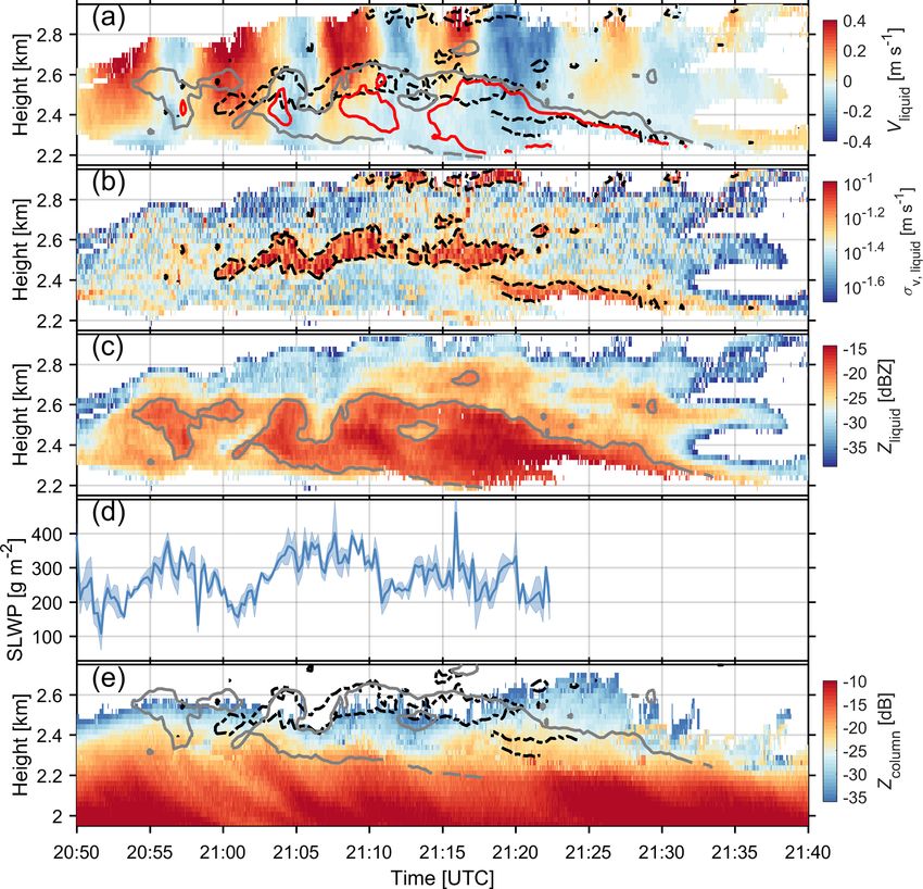
13594                                                    H. Li et al.: Supercooled liquid water and secondary ice production

ondary ice production (SIP) mechanisms that explain the pro-       ume Shupe et al. (e.g., 2004); Luke and Kollias (e.g., 2013).
duction of additional ice particles (e.g., Hallett and Mossop,     The utilization of the polarimetric spectral analysis technique
1974; Lauber et al., 2018; Field et al., 2017). Their impor-       (Spek et al., 2008; Moisseev et al., 2015; Luke et al., 2010;
tance and occurrence, however, is still a topic of current sci-    Oue et al., 2015; Kalesse et al., 2016; Li and Moisseev, 2020;
entific interest (Field et al., 2017; Korolev et al., 2020; Mor-   Luke et al., 2021; Li et al., 2021) allows for the identification
rison et al., 2020; Shaw et al., 2020; Luke et al., 2021).         of supercooled liquid water, which is indicative of vertical
   The existence of supercooled liquid water in mixed-phase        air motions, and ice columns, thereby facilitating the analy-
clouds necessitates the sufficient supply of water vapor to re-    sis of different hydrometeor populations and vertical air mo-
plenish its depletion due to ice particles. For single-layered     tions simultaneously. In this study, this data analysis method
mixed-phase clouds, the water vapor supply may benefit             is used to uncover the K–H billows of supercooled liquid wa-
from a number of processes (Morrison et al., 2012) such as         ter and ice columns embedded in a stratiform precipitation
the adiabatic cooling of air parcels due to turbulence (Ko-        event.
rolev and Field, 2008) and cloud-scale updrafts (Shupe et al.,        The paper is organized as follows: Sect. 2 introduces the
2008b), radiative cooling of the liquid cloud layer (Pinto,        data used in this study; an overview of a stratiform precip-
1998), entrainment of upper moist air (Solomon et al., 2011),      itation event is shown in Sect. 3; Sect. 4 demonstrates the
and feedbacks with the surface (Morrison and Pinto, 2006).         methods used to analyze this event; the dynamics and mi-
While multilayered clouds, where a supercooled liquid water        crophysics of embedded K–H billows are shown in Sect. 5;
layer is embedded in an ice-precipitating cloud, occur fre-        and discussions and conclusions are given in Sects. 6 and 7,
quently (Shupe et al., 2006; Intrieri et al., 2002) and may        respectively.
produce drizzle-sized drops (Majewski and French, 2020) as
well as secondary ice particles (Hallett and Mossop, 1974;
Lauber et al., 2018; Luke et al., 2021), they are much less        2   Measurements
studied owing to the complexity of the microphysical pro-
cesses that are taking place.                                      In this study, measurements from several radars supple-
   Past studies have highlighted the importance of upward          mented by radiosonde observations are used to study mi-
air motions, such as shear-induced turbulence (Hill et al.,        crophysical and dynamical properties of a stratiform pre-
2014), orographic forcing (Lohmann et al., 2016) and pe-           cipitation event that took place on 18 April 2018. The ver-
riodic supersaturation variations (Korolev, 1995; Majewski         tically pointing C- and W-band radars (HYDRA-C and -
and French, 2020), for the growth of liquid droplets in mul-       W) deployed at the University of Helsinki’s Hyytiälä sta-
tilayered mixed-phase clouds. In addition to these mecha-          tion (61.845◦ N, 24.287◦ E) (Hari and Kulmala, 2005; Petäjä
nisms, isobaric mixing (Korolev and Isaac, 2000) and in-           et al., 2016) are aided by a scanning weather radar. This radar
homogeneous mixing (Pobanz et al., 1994), which usually            setup provides various observing views over Hyytiälä, facil-
take place in dynamically unstable regions such as Kelvin–         itating the synthetic analysis of clouds and precipitation (Li
Helmholtz (K–H) clouds, seem to also favor the formation of        et al., 2020; Sinclair et al., 2016). The closest sounding sta-
large supercooled droplets. However, there seems to be a lack      tion to the Hyytiälä station is located at Jokioinen, which is
of observations with a detailed depiction of vertical air mo-      around 123 km to the southwest of Hyytiälä. The sounding is
tions, which are critical for analyzing the driver of the mix-     launched twice a day at around 00:00 and 12:00 UTC. The ra-
ing process (Majewski and French, 2020). Aircraft measure-         diosonde observations at 23:30 UTC (the 00:00 UTC sound-
ments have been widely utilized for analyzing the growth of        ing) were used in our analysis
liquid drops in mixed-phase clouds (e.g., Korolev and Isaac,          Both vertically pointing radars, HYDRA-C and -W, oper-
2000; Hogan et al., 2002; Majewski and French, 2020); how-         ate in the linear depolarization ratio (LDR) mode. HYDRA-
ever, they are only available along the aircraft tracks and can-   C is a container-based weather radar that was transported
not resolve the vertical profiles of different hydrometeors. To    to Hyytiälä in the summer of 2016. Prior to its deployment
provide a larger-scale view of the clouds, radar observations      at the Hyytiälä station, HYDRA-C was operating in Jär-
are often used (e.g., Petre and Verlinde, 2004; Barnes et al.,     venpää (Moisseev et al., 2015). HYDRA-W is a frequency-
2018; Luce et al., 2012; Geerts and Miao, 2010; Houser and         modulated continuous-wave radar (Küchler et al., 2017) and
Bluestein, 2011; Medina and Houze Jr, 2016; Conrick et al.,        has been deployed at the Hyytiälä station since November
2018; Grasmick and Geerts, 2020; Gehring et al., 2020). Be-        2017.
cause radar observations are more sensitive to larger hydrom-         The Doppler radar moments (e.g., reflectivity, LDR,
eteors, it is often impossible to separate echoes from ice par-    Doppler velocity and spectral width) were recorded by both
ticles and water droplets at the same time.                        radars. The pulse length of HYDRA-C is 0.5 µs, resulting in
   For vertically pointing radars, the recorded Doppler spec-      a range resolution of 75 m, which was oversampled to 50 m.
tra split radar returns over a range of sampled Doppler veloc-     HYDRA-W employs dynamic range resolutions of 25.5 and
ities (Kollias et al., 2011) and can be used to separate echoes    34 m for range gates lower and higher than 3577 m, re-
from different hydrometeor types in a radar sampling vol-          spectively. The Doppler spectra of HYDRA-W were calcu-

Atmos. Chem. Phys., 21, 13593–13608, 2021                                          https://doi.org/10.5194/acp-21-13593-2021
H. Li et al.: Supercooled liquid water and secondary ice production                                                          13595

lated by applying a fast Fourier transform with 1024 points         wind shear layer, a region of enhanced spectral width, as can
(Vmax, W = 10.24 m s−1 ) below and 512 points (Vmax, W =            be seen in Fig. 1b, is present between 21:00 and 21:50 UTC.
5.12 m s−1 ) above 996 m. The spectral compression mode             From 20:20 through 21:20 UTC, the HYDRA-W-measured
was used for HYDRA-W and the background noise was re-               mean Doppler velocity exhibits visible oscillations between
moved by applying a noise filter factor that is character-          2.3 and 3.2 km (Fig. 1c), implying the presence of an embed-
ized by the standard deviation of the Doppler spectrum. The         ded convection.
archived W-band polarimetric spectra data enable the analy-            To verify if the environmental conditions were favorable
sis of spectral LDR. The time resolutions of HYDRA-C and            for the formation of the K–H instability, the radio sounding
-W are 1.37 and 3.35 s, respectively. All observations were         data were used. Observations from the radiosonde launched
binned into the time resolution of HYDRA-C and the range            at 23:30 UTC on 18 April 2018 are shown in Fig. 2. The
resolution of HYDRA-W. The beam widths of HYDRA-C                   Richardson number (Ri) was computed in both dry and moist
and -W are 0.48 and 1◦ , respectively.                              conditions following the method used by Hogan et al. (2002).
   Most of the presented analysis is based on HYDRA-W               The air between 0.3 and 3.1 km was almost saturated, and the
observations. The C/W dual-wavelength observations at the           moist Ri from 1.7 to 3.5 km was mostly below 0.25, indicat-
cloud top were used to compute the path-integrated attenua-         ing that the necessary conditions for the development of the
tion (Li and Moisseev, 2019; Tridon et al., 2020). This atten-      K–H instability were met.
uation was then used to estimate the supercooled liquid water          Because the radio sounding station is not very close to
path (SLWP) (Hogan et al., 2005).                                   Hyytiälä, the Doppler velocity observations from Ikaalinen
   The scanning C-band dual-polarization weather radar is           radar were used as additional auxiliary information to sup-
located in Ikaalinen (IKA), 64 km west of Hyytiälä sta-             port the hypothesis of the formation of the K–H instability.
tion, and is operated by the Finnish Meteorological Institute       From the RHI measurements, vertical profiles of the Doppler
(FMI). The Ikaalinen C-band radar performs range–height             velocity observations above the station were extracted. The
indicator (RHI) scans over Hyytiälä every 15 min. As part           time series of these profiles is shown in Fig. 1d and e. One
of the data analysis, the Ikaalinen radar raw data were pro-        can observe that IKA radial velocity observations detect a
cessed using the Python ARM Radar Toolkit (Helmus and               wind shear of 1–2 m s−1 (km−1 ) in the region where the ver-
Collis, 2016). In this study, the Doppler velocity observations     tical velocity oscillations occur. This wind shear is strongest
of Ikaalinen radar were employed to identify the radial wind        between 20:40 and 21:40 UTC. It more or less disappears af-
shear over the Hyytiälä station.                                    ter that. The observed duration of the wind shear is an im-
   As the Ikaalinen radar is routinely calibrated, its reflec-      portant observation that potentially explains the evolution of
tivity measurements were also used to calibrate HYDRA-C.            the K–H billows, as will be discussed below. We should also
The calibration of HYDRA-W was then cross-checked by                point out that the snow-generating cells, clearly visible in
matching HYDRA-C and HYDRA-W reflectivity values at                 Fig. 1a, may affect stability of the layer where we believe the
cloud tops where the Rayleigh approximation applies at both         oscillations have formed. This, in turn, may affect the prop-
bands (Hogan et al., 2005; Kneifel et al., 2015; Falconi et al.,    erties of the K–H instability, and it may not have a “classic”
2018; Li and Moisseev, 2019; Tridon et al., 2020).                  appearance. However, the correlation between the K–H in-
                                                                    stability and wind shear indicates that shear may play a dom-
                                                                    inant role in formation of the K–H wave.
3   Overview of the event

A stratiform precipitation system passed over Hyytiälä be-          4     Methods
tween 17:00 UTC on 18 April and 04:00 UTC on 19 April
2018. The time–height evolution of this stratiform precipita-       4.1    HYDRA-W Doppler spectra analysis
tion captured by HYytiälä Doppler RAdar-W (HYDRA-W;
Li and Moisseev, 2020) between 20:00 and 22:30 UTC on               In a radar volume, hydrometeors with different fall veloci-
18 April 2018 is presented in Fig. 1a, b and c. As shown            ties are typically present. Multilayered mixed-phase clouds
in Fig. 1a, the precipitation intensifies after 21:45 UTC. C-       are a good example of conditions where hydrometeors with
band radar reflectivity at 400 m (not shown) increased from         diverse fall velocities are present in a radar volume (Ram-
∼ 5 to ∼ 20 dBZ with the rain rate increasing from 0.1 to           bukkange et al., 2011; Verlinde et al., 2013; Kalesse et al.,
0.7 mm h−1 . During the presented time period, the cloud top        2016). In such cases, the analysis of Doppler radar spec-
stays at ∼ 4 km, where the air temperature is around −15 ◦ C.       tra measured by a vertically pointing radar can be used to
The snow-generating cells at the cloud top can be identified        separate radar echoes of these particles. The sizes of typical
by the positive Doppler velocities (Fig. 1c). About 1 km be-        supercooled liquid droplets range from 5 to 20 µm (Shupe
low the radar-detected cloud top, the fall streaks visible in the   et al., 2008b). The terminal velocities are in the order of 0.03
reflectivity observations change their direction, indicating the    and 0.07 m s−1 for 10 and 50 µm liquid droplets, respectively
presence of a wind shear layer. It is noteworthy that below the     (Kollias et al., 2001). Given their negligible fall velocities,

https://doi.org/10.5194/acp-21-13593-2021                                           Atmos. Chem. Phys., 21, 13593–13608, 2021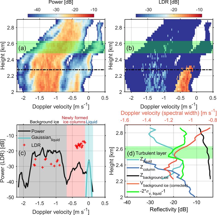
13596                                                        H. Li et al.: Supercooled liquid water and secondary ice production

Figure 1. Radar observations collected on 18 April 2018 between 20:00 and 22:30 UTC showing vertically pointing HYDRA-W reflectiv-
ity (a), spectral width (b) and mean Doppler velocity (c). Panels (d) and (e) present vertical profiles of radial Doppler velocity and vertical
wind shear derived from the range–height indicator (RHI) scans of Ikaalinen radar (IKA), respectively. Purple and black contours depict the
wind shear of −1 and 1 m s−1 (km−1 ), respectively. The 0 and −10 ◦ C isotherms are marked by gray dashed lines. The black dashed box
shows the region where the spectral analysis has identified the presence of supercooled liquid, as shown in Fig. 4.

these cloud droplets can be used as tracers for air motions.              2013; Spek et al., 2008). In some cases, the presence of new
In Doppler radar spectra, the radar returns from liquid cloud             ice particles is indicative of SIP (Zawadzki et al., 2001). At
droplets can be identified as a narrow peak around 0 m s−1 .              vertical incidence, LDR can be used to discriminate between
The mean velocity of this peak can be used to derive vertical             columns and other types of ice (Matrosov, 1991; Matrosov
air motion (Shupe et al., 2004).                                          et al., 1996; Oue et al., 2015; Li et al., 2021). The columnar
   In multilayered mixed-phase clouds, more than one popu-                crystals will produce LDR values as large as −16 to −13 dB.
lation of ice may exist (Zawadzki et al., 2001; Verlinde et al.,          Figures 3a and b present vertical profiles of W-band radar

Atmos. Chem. Phys., 21, 13593–13608, 2021                                                   https://doi.org/10.5194/acp-21-13593-2021
H. Li et al.: Supercooled liquid water and secondary ice production                                                               13597

                                                                         by a Gaussian model (Luke and Kollias, 2013). If individ-
                                                                         ual Doppler spectra of different particles can be modeled
                                                                         using Gaussian shapes, their spectral moments can be esti-
                                                                         mated using Gaussian mixture models (Nguyen et al., 2008).
                                                                         However, the Doppler spectra of ice particles do not neces-
                                                                         sarily follow this functional form. Nevertheless, the Gaussian
                                                                         model is a good approximation for the Doppler spectrum of
                                                                         liquid cloud droplets (Luke and Kollias, 2013). As the right
                                                                         slope of the liquid cloud droplet mode in the Doppler spec-
                                                                         trum is less affected by the ice mode, the Gaussian model can
                                                                         still be fitted to the right part of the cloud droplet spectrum
                                                                         (Luke and Kollias, 2013). As shown in Fig. 3c, the Gaussian
                                                                         model fits the spectral peak of supercooled liquid water well.
                                                                         Using such a Gaussian fit, the reflectivity, spectral width and
                                                                         Doppler velocity of supercooled liquid water were derived.
                                                                         The reflectivity of the columnar ice mode in the Doppler
                                                                         spectrum was calculated directly from the spectrum, as we
                                                                         expect that the impact of the liquid mode on the reflectivity
                                                                         of columnar ice is not significant enough to affect our study
                                                                         of the evolution of ice columns (Oue et al., 2015; Kalesse
                                                                         et al., 2016).
Figure 2. Radiosonde observations at 23:30 UTC on 18 April 2018
from the Jokioinen station. This figure shows the air temperature (T ,
red line), relative humidity (RH, blue line), and dry (green cross)      4.2   Estimation of the supercooled liquid water path
and moist (black circle) Ri numbers derived from the radiosonde
data. The vertical black line indicates the critical Richardson num-     The retrieval of the SLWP was mainly based on the dif-
ber Ri = 0.25. The gray shaded area in this figure corresponds to        ferential attenuation between C- and W-band radar reflec-
the heights as marked by the black dashed box in Fig. 1.                 tivity (Hogan et al., 2005).This event was observed by
                                                                         two radars, namely W-band cloud and C-band precipitation
                                                                         radars. While the attenuation due to rain, the melting layer,
Doppler spectral power and LDR, respectively. The super-                 ice particles and supercooled liquid water is negligible for the
cooled liquid water, with relatively weak and narrow spec-               C-band radar signal, it may have a strong impact on W-band
tral mode (Shupe et al., 2004, 2008b; Luke et al., 2010),                radar observations (Hogan et al., 2005; Li and Moisseev,
exists between 2.2 and 2.85 km. Ice crystals with a spec-                2019). The differential attenuation between C- and W-band
tral LDR around −15 dB and Doppler velocity lower than                   radar observations caused by supercooled liquid water is pro-
0.8 m s−1 are attributed to the columnar ice (Oue et al., 2015).         portional to the liquid water content (Hogan et al., 2005).
The spectral power of the background ice falling from up-                Therefore, if the attenuation due to other attenuation sources
per clouds is much larger than that of liquid water droplets             can be mitigated, the differential attenuation measurements
and ice columns. A close-up of the measurements at a height              can be used to estimate the SLWP.
of 2.28 km is shown in Fig. 3c. The background ice, newly                   For HYDRA-W, the observed reflectivity is affected by the
generated ice columns and supercooled liquid in the Doppler              attenuation from the atmosphere and the wet radome. Us-
spectrum are shown using gray, yellow and blue shading, re-              ing the reflectivity observations from HYDRA-C, the atmo-
spectively. As can be seen, the spectral LDR of ice columns              spheric attenuation due to rain and the melting layer at the
is much higher than background ice, whereas the LDR sig-                 W-band was removed by applying reflectivity–attenuation re-
nals for supercooled liquid water are below the noise level.             lations (Li and Moisseev, 2019). It was found that the atten-
   The Doppler spectra components of different hydrome-                  uation due to rain and the melting layer is relatively small,
teor types, present during this event, can be identified using           less than 1 dB, and the uncertainties in attenuation estimation
Doppler velocity and spectral LDR, as discussed above. De-               were, in the order of 0.5 dB (Li and Moisseev, 2019). Given
spite the straightforward identification of different ice parti-         the weak rain intensity, the attenuation due to ice particles
cle types in the Doppler spectrum, deriving their spectral mo-           is negligible (Leinonen et al., 2011). The gaseous attenua-
ments, like reflectivity, Doppler velocity and spectral width,           tion can be calculated from the Millimeter-wave Propagation
is complicated because of the overlap of the spectral modes.             Model (Liebe, 1985). The wet radome attenuation should be
This overlap is enhanced if there is significant spectral broad-         minimized, as the antenna of HYDRA-W is protected by a
ening due to the horizontal and vertical wind shears, and tur-           hydrophobic cover and the blower further reduces radome
bulence. As the size distribution of liquid droplets is rela-            wetting. After the attenuation due to rain and the melting
tively narrow, their spectrum can be closely approximated                layer was removed from W-band reflectivity, the differential

https://doi.org/10.5194/acp-21-13593-2021                                              Atmos. Chem. Phys., 21, 13593–13608, 2021
13598 H. Li et al.: Supercooled liquid water and secondary ice production
Figure 3. Vertical Doppler spectra profiles at 21:08:43 UTC for (a) power and (b) LDR. Panel (c) presents a zoomed-in view of the spectral
power and LDR as marked by the dot-dash lines in panels (a) and (b). Panel (d) presents vertical profiles of the scaled spectral width of the
supercooled liquid water mode (green line) in the Doppler spectra (σv, liquid ), the Doppler velocity of background ice (Vbackground ice ) after
correcting air motions retrieved from liquid water, and radar reflectivity of supercooled liquid water (Zliquid ), columnar ice (Zcolumn ) and
background ice (Zbackground ice ). The gray, red and blue shaded areas in panel (c) indicate background ice from above, newly formed ice
columns and supercooled liquid, respectively. The green shaded areas in panels (a), (b) and (d) indicate the turbulent layer as characterized
by the increased σv, liquid . Negative velocity indicates downward.
attenuation was derived by matching C- and W-band reflec- mentioned figure panels depicts the region where the super-
tivities at the cloud top, where ice particles are expected to be cooled liquid water was detected. The Doppler analysis was
small enough to satisfy the Rayleigh approximation in both also performed on the regions outside of the rectangle, but no
radar bands. The SLWP was then converted from the differ- supercooled water or columnar ice production was detected
ential attenuation which is mainly caused by the liquid atten- there.
uation at W-band (Hogan et al., 2005).
5.1 Doppler velocity and the spectral width of
5 The Kelvin–Helmholtz billows supercooled liquid water
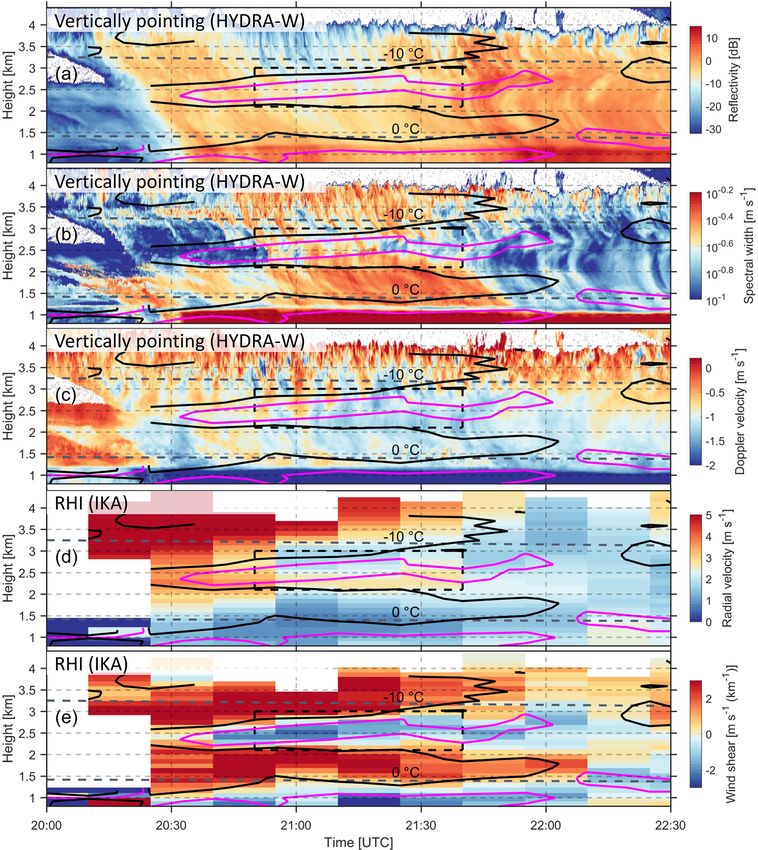
The following discussion is focused on the analysis of dy- A layer of supercooled liquid water persisted during the en-
namics and microphysical properties of the cloud region tire period (Fig. 4). As the cloud droplet fall velocity does not
inside the black rectangle in Fig. 1a, b and c (20:50– usually exceed a few centimeters per second (∼ 0.03 m s−1
21:40 UTC). This period will be analyzed with the help of for the diameter of 10 µm), Vliquid is used for the assessment
specifically derived radar reflectivity (Zliquid ), spectral width of the vertical velocity of air motion (Shupe et al., 2004).
(σv, liquid ) and Doppler velocity of the supercooled liquid wa- Figure 4a reveals periodic air circulations with the ampli-
ter (Vliquid ); reflectivity of ice columns (Zcolumn ); and the tude of approximately 0.4 m s−1 . It should be noted that the
SLWP. It should be noted that the rectangle in the above- K–H instability may not be the only factor modulating air
Atmos. Chem. Phys., 21, 13593–13608, 2021 https://doi.org/10.5194/acp-21-13593-2021H. Li et al.: Supercooled liquid water and secondary ice production 13599 Figure 4. The (a) Doppler velocity, (b) spectral width and (c) reflectivity of supercooled liquid cloud droplets, (d) the SLWP above the melting layer estimated from the differential attenuation between C- and W-bands, and (e) the reflectivity of ice columns are shown. The blank regions in panels (a), (b), (c) and (e) are where no significant supercooled liquid mode (a, b, c) or columnar ice mode (e) can be identified in the radar Doppler spectrum. Red and gray isolines indicate the reflectivity of −18 and −21 dBZ for supercooled liquid water, respectively. Black dashed isolines indicate the spectral width of 0.06 m s−1 for supercooled liquid water. The shaded areas in panel (d) indicate the standard deviation of the SLWP in 13.7 s. After 21:23 UTC, no SLWP retrieval was made. This was caused by the rapid changes in the observed C-band reflectivity at cloud top, which hindered the identification of Rayleigh scattering regions. motions, since the wind shear layer is so close to the cloud billows and vertical air motions bears a good resemblance to top. However, we argue that the oscillation of air motions previous vertically pointing radar records of K–H clouds (Pe- at around 2.8 km is mainly caused by the K–H instability. tre and Verlinde, 2004; Geerts and Miao, 2010; Luce et al., Firstly, the wind shear layer, which is inductive to vertical 2012). Despite the lower amplitude of the vertical velocities air motions, at 2.8 km was clearly present from 20:50 to in the present observations, both temporal (∼ 5 min) and spa- 21:40 UTC (Fig. 1e). Secondly, after 22:00 UTC, when the tial (∼ 300 m) scales of each wave are very similar to those wind shear layer has almost disappeared, there are no identi- K–H billows observed in the convective outflow anvil (Petre fiable signatures of air oscillations at 2.8 km (Fig. 1c). and Verlinde, 2004). In addition, σv, liquid is enhanced along A wave train of enhanced σv, liquid at around 2.5 km is colo- the central axis (Barnes et al., 2018) rather than only around cated with vertical air perturbations (Fig. 4b). Specifically, the crests of K–H waves (Houser and Bluestein, 2011). the upward branches of the waves coincide with updrafts, The enhanced σv, liquid can be caused by the broadening of and the crests of waves are close to the transitional regions the drop size distribution as well as the enhanced turbulence of upward and downward velocities. Such colocation of K–H within the radar volume. If it was attributed to the former, the https://doi.org/10.5194/acp-21-13593-2021 Atmos. Chem. Phys., 21, 13593–13608, 2021
13600 H. Li et al.: Supercooled liquid water and secondary ice production
increase in σv, liquid would not be only 100 to 200 m in depth Interestingly, several fall streaks of ice columns present be-
and would not vanish just below 2.4 km. Therefore, we con- low the K–H billows, and each of them (around 21:04, 21:10
clude that the sharp increase in σv, liquid was mainly caused and 21:22 UTC, respectively) corresponds to a crest in the K–
by the velocity fluctuations and that mixing was taking place H billows as indicated by the enhanced Zliquid and σv, liquid .
between 2.4 and 2.6 km.
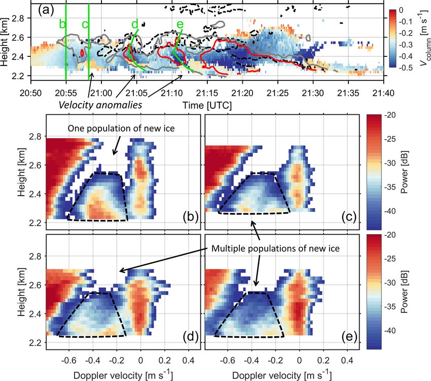
5.5 Multiple populations of ice columns
5.2 Reflectivity of supercooled liquid water
Based on the air motions estimated from the Vliquid , we have
The regions of enhanced Zliquid manifest themselves as well- been able to estimate the terminal Doppler velocity of ice
defined K–H billows (see the gray solid isolines in Fig. 4c), columns (Vcolumn ), as shown in Fig. 5a. Before 20:56 UTC,
especially between 21:00 and 21:13 UTC. The crests of the Vcolumn increases as ice columns fall toward the ground. This
K–H billows are around the transitional regions of upward is expected, as the mass of ice columns increases during
and downward velocities and protrude to downdrafts. Just riming (if they are not too small) and depositional growth,
below the turbulent layer, as characterized by the increased leading to increased terminal velocity (Lamb and Verlinde,
σv, liquid , there is a region of enhanced Zliquid which is as 2011). After 20:56 UTC, an intermittent slowdown of Vcolumn
high as −16 dBZ, indicating the onset of drizzle in this re- at around 2.3 km occurred (black arrows). This anomalous
gion (Frisch et al., 1995). decrease in Vcolumn is surprising, given the fact that the air
Interestingly, the K–H billows of Zliquid (gray solid iso- motion has already been corrected. In addition, the velocity
lines) are colocated with the enhanced σv, liquid (black dashed anomalies are well colocated with the areas of high Zliquid
isolines), as shown in Fig. 4a. This colocation resembles (above −18 dBZ, red isolines).
what has been observed in rain where the perturbation from Further inspection of the radar Doppler spectra observa-
the K–H instability is expected to facilitate the coalescence tions was carried out. Figure 5b, c, d and e show the observed
of raindrops and leads to increased radar reflectivity (Barnes Doppler spectral power of the green lines labeled b, c, d and e
et al., 2018). in Fig. 5a, respectively. The green lines labeled d and e were
Previous observational studies have shown that K–H bil- identified by tracing the peaks of Zliquid . It is anticipated that
lows embedded in precipitation can be characterized by the the green lines are representative of the quasi-Lagrangian tra-
fluctuations in radar reflectivity and spectral width colocat- jectories of ice columns. As expected, there seems to be one
ing with Doppler velocities (Petre and Verlinde, 2004; Geerts population of ice columns in Fig. 5b that corresponds to the
and Miao, 2010; Barnes et al., 2018). In this event, such sig- period with no velocity anomaly. In contrast, multiple popu-
natures are hardly identifiable in conventional radar reflec- lations of ice columns can be identified in Fig. 5c, d and e.
tivity and spectral width observations (Fig. 1a, b), despite the At a height of 2.3 km, the velocity of faster falling columnar
evidence of air circulations as indicated by mean Doppler ve- ice is 0.5–0.6 m s−1 , whereas the velocity of slower falling
locities (Fig. 1c). This difference may be explained by much columnar ice is 0.2–0.3 m s−1 . Figure 5d and e suggest that
weaker vertical air motions and the potential impact of snow- the generation of the faster falling ice columns coincides with
generating cells at the cloud top in this study. the turbulent layer at around 2.55 km, whereas the slower
ones were formed at around 2.4 km, which corresponds to
5.3 Supercooled liquid water path the region of enhanced Zliquid .
As shown in Fig. 4d, the SLWP presents a wave-like pat-
tern as well. The estimated SLWP ranges from 150 to 6 Discussion
400 g m−2 between 21:00 and 21:15 UTC. In general, the
SLWP is larger in downdrafts than in updrafts, somewhat 6.1 Generation of large droplets
resembling aircraft observations presented by Majewski and
French (2020). The oscillations in the SLWP and observed As shown in Fig. 4c, the reflectivity of supercooled liq-
supercooled liquid droplet velocities do not fully coincide. uid water can be as high as −18 to −15 dBZ, which ex-
This discrepancy can be attributed to presence of supercooled ceeds (or is close to) the expected reflectivity of drizzle, e.g.,
liquid at the other altitudes, i.e., at around 1.5 km (not shown) −20 dBZ (Kato et al., 2001), −17 dBZ (Kogan et al., 2005)
and potentially at the top of the snow-generating cells. and −15 dBZ (Chin et al., 2000). Generally, the reflectivity of
liquid clouds seldom exceeds −18 dBZ (Frisch et al., 1995).
5.4 Generation of ice columns Thus, this indicates the onset of drizzle that is taking place in
the K–H billows.
Zcolumn was derived from the columnar ice mode in radar One of the striking observations is that the level where
Doppler spectrum observations. As shown in Fig. 4e, the de- velocity oscillations are most intensive is obviously higher
tected ice columns initiate at about 2.5 km, coinciding with than the regions of enhanced reflectivity of supercooled liq-
the enhanced σv, liquid . Once generated, these ice particles uid water. This suggests that droplet growth at quasi-steady
grow rapidly from about −30 to −15 dBZ within ∼ 0.3 km. supersaturation formed in adiabatically ascending cloud is
Atmos. Chem. Phys., 21, 13593–13608, 2021 https://doi.org/10.5194/acp-21-13593-2021H. Li et al.: Supercooled liquid water and secondary ice production 13601 Figure 5. (a) The Doppler velocity of ice columns after the air motion correction. For the green lines labeled (b), (c), (d) and (e), the corresponding Doppler spectral power observations after the air motion correction are shown in panels (b), (c), (d) and (e), respectively. Red and gray isolines in panel (a) indicate the reflectivity of −18 and −21 dBZ for supercooled liquid water, respectively. Black dashed isolines in panel (a) indicate the spectral width of 0.06 m s−1 for supercooled liquid water. Black arrows point to the regions of velocity anomalies in panel (a). Populations of new ice in panels (b), (c), (d) and (e) are marked by black dashed curves. not the only mechanism responsible for drizzle formation 2000) which is favorable for the generation and growth of (Houze Jr and Medina, 2005; Shupe et al., 2008b; Houser and supercooled liquid droplets. Although the observed inversion Bluestein, 2011; Morrison et al., 2012). Given the apparent over the radiosonde station is relatively weak and the temper- presence of enhanced turbulence (Fig. 4b), we speculate that ature difference between the air masses below and above the drizzle formation could be associated with isobaric mixing. inversion is around 1.5 ◦ C, we speculate that the actual inver- The supersaturation caused by isobaric mixing of saturated sion over the Hyytiälä station might be stronger. air parcels with different temperatures can facilitate the gen- The inhomogeneous mixing in the K–H instability can eration of drizzle (Korolev and Isaac, 2000). Figure 2 shows also contribute to the generation of large supercooled the presence of the inversion around 1.5 ◦ C embedded in the droplets (Pobanz et al., 1994). As soon as the liquid droplets liquid layer at ∼ 2.75 km. Vertical transport of cloud parcels meet with dry air, they evaporate until saturation is reached or forced by the wind shear to the levels below and above the until liquid water is depleted. This mixing process facilitates inversion will result in temperature fluctuations in a saturated the formation of large droplets due to the depletion of small environment required for the generation of cloud volumes liquid droplets; hence, more excess water vapor is available with high supersaturation formed due to isobaric mixing. The to grow large cloud droplets (Lamb and Verlinde, 2011). The mixing process is supported by the enhanced spectral width circulation of this process allows for the continuous growth (Fig. 4b) which is indicative of strong sub-radar-volume ve- of liquid droplets (Korolev, 1995), as supported by recent air- locity fluctuations. The colocation of the enhanced spectral craft observations (Majewski and French, 2020). After over- width and reflectivity further indicates the strong link be- coming the mechanistic gap around the diameter of 40 µm tween the mixing and large-drop formation. The relatively (Lamb and Verlinde, 2011), these liquid drops grow more ef- high SLWP values during downdrafts seem to further corrob- ficiently during the collision–coalescence process (Korolev orate this hypothesis. The temperature fluctuation of 2.5 ◦ C and Isaac, 2000). can lead to a supersaturation of 0.5 % (Korolev and Isaac, https://doi.org/10.5194/acp-21-13593-2021 Atmos. Chem. Phys., 21, 13593–13608, 2021
13602 H. Li et al.: Supercooled liquid water and secondary ice production
6.2 Secondary ice production breakup during freezing (Field et al., 2017; Lauber et al.,
2018, 2021; Keinert et al., 2020). Activation of the H–M pro-
As follows from Fig. 4, the first radar echo of ice columns cess requires a set of necessary conditions: (a) the presence of
was detected at approximately 2.5–2.6 km. As ice crystals droplets larger than 24 µm, (b) an environmental temperature
must grow for some time in order to become detectable by of −8 to −3 ◦ C and (c) the presence of rimed snow flakes. As
the radar, the actual level of the columns’ origin is most likely follows from the discussion above, conditions (a) and (b) are
located at the top of the mixed-phase layer at 2.65 km. The satisfied in the mixed-phase layer. The presence of graupel
temperature at this altitude was around −8 ◦ C, which is ex- and heavily rimed ice is supported by the observed Doppler
pected for the columnar growth. During their fall through the velocity (around 2 m s−1 after compensating for air motions;
mixed-phase layer, the columns grew and the average fall ve- Fig. 3a). Therefore, the environmental conditions required
locity reached approximately 0.35 m s−1 , as derived from the for the initiation of the H–M process were satisfied in the
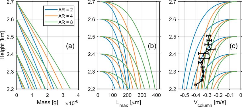
Doppler spectrum at 2.2 km. To assess the back trajectory of mixed-phase layer. The presence of drizzle-sized drops and
ice crystals, a simulation of free-falling growing ice columns background ice is also favorable for SIP via droplet breakup
was performed (see the Appendix). In this simulation, the during freezing (Lauber et al., 2018; Keinert et al., 2020).
cloud environment was considered to be saturated over liq- This is very possible given that Luke et al. (2021) recently
uid water. proposed that droplet breakup is more efficient than the H–
Figure 6 shows the modeled changes in mass, maximum M process in natural clouds. The background ice particles in
length (Lmax ) and Vcolumn between 2.2 and 2.7 km for colum- this case can play the role of INPs. Hence, it is concluded
nar crystals with aspect ratios of 2, 4 and 8. The radar ob- that both mechanisms may be responsible for the observed
served Vcolumn between 21:08:20 and 21:08:50 UTC during SIP.
which one population of ice columns presented was used For the first time, multiple populations of newly generated
for the assessment (black curve in Fig. 6c). In order for the ice particles have been identified in K–H billows. The spec-
simulated Vcolumn to be consistent with radar measurements, tral analysis method presented in study shows the potential
the aspect ratio (AR) of ice columns formed at 2.6–2.7 km of remote sensing techniques for studying the evolution of a
should be 4–8, which implies that the mass of these columns SIP event. In particular, although the spatially separated SIP
(m) was 2–3×10⁻⁶ g at around 2.2 km. At this level, Zcolumn cloud regions can be identified from the “needle-like” air-
(Fig. 3d) is −15 to −18 dB. Hence, the ice water content craft penetrations (e.g., Hogan et al., 2002; Korolev et al.,
of ice columns (IWC) was 0.009–0.014 g m−3 based on the 2020), our understanding of their distribution is rather lim-
parameterization IWC = 0.167Z 0.712 , derived using aircraft ited (Field et al., 2017). Summarizing the obtained observa-
observations within the temperature range of −12 to −3 ◦ C tions, it could be stated that K–H instability embedded in a
(Korolev et al., 2020). Therefore, the number concentration relatively deep mixed-phase layer may create conditions fa-
of ice columns (N = IWC/m) is in the range of 3–8 L−1 . In- vorable for enhanced growth of large droplets, which facil-
terestingly, the N estimated from the temperature-dependent itate the initiation of SIP. Several past observations suggest
IWC-Z parameterization (Hogan et al., 2006) is within the that, in many cases, SIP was spatially associated with dy-
same magnitude (4.7 ± 3.7 L−1 for Zcolumn of −10 dB at namically active cloud regions (Korolev et al., 2020; Lasher-
2 km, −5 ◦ C). The estimated primary INPs based on the Trapp et al., 2016; Rauber et al., 2019). The present study
parameterization of DeMott et al. (2010) is about 0.3 L−1 supports this previously attained finding. As a result, we ad-
at −8 ◦ C. The INP parameterization from Schneider et al. vocate that more efforts should be devoted to addressing the
(2021) derived from measurements obtained at the Hyytiälä microphysical impact of SIP, as currently poorly parameter-
station yields the primary INP concentration of 7×10⁻⁴ L−1 ized in models (Morrison et al., 2020), associated with the
at −8 ◦ C. These values are about 1–5 orders of magnitude K–H instability.
lower than the estimated ice number concentration. There-
fore, the estimated concentration of columns cannot be ex-
plained by primary nucleation. In addition, their origin in the
mixed-phase layer cannot be explained by the seeding ice 7 Conclusions
from above, as the columnar shape is not consistent with the
environmental conditions in the cloud above. As a result, SIP On 18 April 2014 between 20:50 and 21:40 UTC, a K–H
is the most likely explanation for the observed columnar ice. cloud embedded in stratiform precipitation was observed
Considering that smaller ice columns contribute less to the over the University of Helsinki measurement site in Hyytiälä,
radar reflectivity, the actual concentration of columns is ex- Finland. The observations were collected using three radars,
pected to be even higher than the estimation. This provides two vertically pointing C- and W-band radars located at the
additional support for ice initiation via SIP. site and a scanning weather radar operated by FMI. The FMI
There are two potential mechanisms to explain SIP in our radar is located 64 km west of the site and performed RHI
observations: the Hallett–Mossop (H–M) process (Hallett scans every 15 min over Hyytiälä. Although oscillations of
and Mossop, 1974; Mossop and Hallett, 1974) and droplet mean vertical Doppler velocity are visible in the data, no ob-
Atmos. Chem. Phys., 21, 13593–13608, 2021 https://doi.org/10.5194/acp-21-13593-2021H. Li et al.: Supercooled liquid water and secondary ice production 13603 Figure 6. Simulated (a) mass, (b) maximum length (Lmax ) and (c) fall velocity (Vcolumn ) of ice columns with aspect ratios (AR) of 2, 4 and 8. Vcolumn was calculated based on the Kajikawa (1976) parameterization. Ice particles were considered to grow at saturation over liquid water. Observations from the radiosonde launched at 23:30 UTC were used as inputs. The radar-observed Vcolumn (black) from 21:08:20 to 21:08:50 UTC is shown in panel (c), and the error bars indicate the standard deviation of Vcolumn during this period. vious signatures of K–H waves were identified from radar Overall, the presented observations and analysis indicate reflectivity and spectral width observations. that even not very strong wind shears may result in the for- To unmask the cloud, radar Doppler spectra analysis was mation of K–H instability, which could lead to the formation performed on the W-band radar observations. The analy- of conditions favorable for the onset of supercooled drizzle sis showed the presence of supercooled cloud embedded in and SIP. the precipitation. The mean Doppler velocities of the cloud droplets, which can be used as tracers of air motion, exhib- ited a well-defined oscillation with a magnitude of 0.4 m s−1 . The FMI weather radar observations detected the presence of a vertical shear layer coinciding with the supercooled liq- uid cloud layer. Given that the lifetime of the cloud coincides with the lifetime of the shear, we speculate that this cloud is mainly formed due to the K–H instability. It should be noted, however, that other processes could also contribute to the for- mation of the atmospheric wave, i.e., air motion associated with the snow-generating cells that are present about 0.5 km above the studied layer. The presented observations and analysis show that K–H clouds are capable of producing large liquid droplets, despite the competition for moisture with ice particles falling from above. In some regions, the observed K–H cloud reflectivity values exceeded −20 dBZ, which is typically associated with the onset of drizzle. Furthermore, spectral linear depolariza- tion ratio observations identified the presence of ice columns. These columns appeared to form in the supercooled liquid cloud regions. In the pockets where larger cloud droplets were formed, multiple populations of columnar ice particles were observed. The estimated number concentration of ice columns is at least 1 order of magnitude higher than the expected concentration of primary ice-nucleating particles. This implies that the secondary ice production is the most likely source of the observed columnar ice. https://doi.org/10.5194/acp-21-13593-2021 Atmos. Chem. Phys., 21, 13593–13608, 2021
13604                                                         H. Li et al.: Supercooled liquid water and secondary ice production

Appendix A

The diffusional growth of columnar ice particles was simu-
lated with the help of an electrostatic approximation of the
ice crystal shapes by capacitance. The mass growth rate was
described as (e.g., Pruppacher and Klett, 1997)
dm 4π CSi fv
   =         .                                                  (A1)
dt   A1 + A2
   Here, Si is the supersaturation over ice, A1 and A2 are
the coefficients dependent on temperature T and pressure
P (e.g., Pruppacher and Klett, 1997), C is the capacitance
equivalent to the particle shape, and fv is the ventilation fac-
tor. The columnar shapes of ice particles were approximated
by prolate spheroids with an aspect ratio of AR = rrba , where
ra and rb are major and minor axes of the prolate spheroid, re-
spectively (ra > rb ). The aspect ratio of the particle remained
constant during simulation. The capacitance of the prolate
spheroid was calculated as
             √
               AR 2 − 1
C = rb           p            .                             (A2)
        ln(AR + AR2 − 1)
  The ventilation factor was calculated as (Wang and Ji,
1992)

fv = 1−0.006681X +2.309X2 +0.734X 3 −0.739X 4 , (A3)
                   1    1
where X = 14 Re 2 Sc 3 . Here, Sc is the Schmidt number, and
                                 ∗
Re is the Reynolds number UvL in which U is the particle
fall velocity and v is the kinematic viscosity. L∗ = ps is the
effective aerodynamic particle size, where s is the surface
area of the prolate spheroid and p is the perimeter of the
maximum projection of the spheroid. Following the observa-
tional study by Kajikawa (1976), the terminal fall velocity of
columnar ice crystals was parameterized as
           0.35
         b P0
U = am              ,                                    (A4)
             P
where P0 = 880 mbar and a and b are dependent on the AR
of columns. Thus, for the calculations, it was assumed that
b = 0.271, a = 2.53 for AR = 2, a = 1.87 for AR = 4, and
a = 1.55 for AR = 8. In Eq. (A4), the particle mass m is in
milligrams (mg) and the fall velocity U is in meters per sec-
ond (m s−1 ). The altitude of falling particles was integrated
from the equation dz = U dt. The temperature profile T as a
function of height z employed in the simulation was adapted
from the observations, as in Fig. 2. As the cloud environment
in the modeling domain (2.2–2.7 km) was in a mixed-phase
state, the water vapor pressure E in this altitude range can be
considered, with high accuracy, to be saturated with respect
to water Esw (Korolev and Mazin, 2003). Therefore, at each
time step, the supersaturation over ice in Eq. (A1) was calcu-
lated as Si = Esw (TE(z))−E   si (T (z))
                      si (T (z))
                                         , where Esi is the saturation
water vapor pressure of ice at T .

Atmos. Chem. Phys., 21, 13593–13608, 2021                                              https://doi.org/10.5194/acp-21-13593-2021
H. Li et al.: Supercooled liquid water and secondary ice production 13605
Data availability. Radiosonde observations can be accessed Barnes, H. C., Zagrodnik, J. P., McMurdie, L. A., Rowe, A. K.,
at http://weather.uwyo.edu/upperair/sounding.html (last access: and Houze Jr, R. A.: Kelvin–Helmholtz Waves in Precipitating
5 July 2020). The radar data used in this study are available at Midlatitude Cyclones, J. Atmos. Sci., 75, 2763–2785, 2018.
https://doi.org/10.5281/zenodo.4019602 (Haoran, 2020). Barrett, A. I., Hogan, R. J., and Forbes, R. M.: Why are mixed-phase
altocumulus clouds poorly predicted by large-scale models?, Part
1. Physical processes, J. Geophys. Res.-Atmos., 122, 9903–9926,
Author contributions. HL and DM conceptualized the study and 2017.
wrote the paper. HL performed the majority of the data analysis. Chin, H.-N. S., Rodriguez, D. J., Cederwall, R. T., Chuang, C. C.,
All the authors took part in the interpretation of the results. AK per- Grossman, A. S., Yio, J. J., Fu, Q., and Miller, M. A.: A mi-
formed the ice particle growth modeling and reviewed and edited crophysical retrieval scheme for continental low-level stratiform
the paper. clouds: Impacts of the subadiabatic character on microphysical
properties and radiation budgets, Mon. Weather Rev., 128, 2511–
2527, 2000.
Competing interests. The authors declare that they have no conflict Conrick, R., Mass, C. F., and Zhong, Q.: Simulated Kelvin–
of interest. Helmholtz waves over terrain and their microphysical implica-
tions, J. Atmos. Sci., 75, 2787–2800, 2018.
DeMott, P. J., Prenni, A. J., Liu, X., Kreidenweis, S. M., Pet-
ters, M. D., Twohy, C. H., Richardson, M., Eidhammer, T., and
Disclaimer. Publisher’s note: Copernicus Publications remains
Rogers, D.: Predicting global atmospheric ice nuclei distribu-
neutral with regard to jurisdictional claims in published maps and
tions and their impacts on climate, P. Natl. Acad. Sci. USA, 107,
institutional affiliations.
11217–11222, 2010.
Falconi, M. T., von Lerber, A., Ori, D., Marzano, F. S., and
Moisseev, D.: Snowfall retrieval at X, Ka and W bands: con-
Special issue statement. This article is part of the special issue “Ice sistency of backscattering and microphysical properties using
nucleation in the boreal atmosphere”. It is not associated with a con- BAECC ground-based measurements, Atmos. Meas. Tech., 11,
ference. 3059–3079, https://doi.org/10.5194/amt-11-3059-2018, 2018.
Field, P., Lawson, R. P., Brown, P. R. A., Lloyd, G., Westbrook,
C.,Moisseev, D., Miltenberger, A., Nenes, A., Blyth, A., Choular-
Acknowledgements. We thank Matti Leskinen for his excellent ton, T., Connolly, P., Buehl, J., Crosier, J., Cui, Z., Dearden,
work on the instrument maintenance. Jussi Tiira is acknowledged C.,DeMott, P., Flossmann, A., Heymsfield, A., Huang, Y., Ka-
for his help in processing radar data. lesse,H., Kanji, Z. A., Korolev, A., Kirchgaessner, A., Lasher-
Trapp, S., Leisner, T., McFarquhar, G., Phillips, V., Stith, J., and
Sullivan, S.: Secondary ice production: Current state of the sci-
Financial support. This research has been supported by the ence and recommendations for the future, Meteorol. Monogr.,
Horizon 2020 project (grant nos. ERA-PLANET – The European 58, 7–1, 2017.
network for observing our changing planet (689443); ACTRIS-2 Frisch, A., Fairall, C., and Snider, J.: Measurement of stratus cloud
– Aerosols, Clouds, and Trace gases Research InfraStructure and drizzle parameters in ASTEX with a Kα-band Doppler radar
(654109); ACTRIS PPP – ACTRIS PPP – Aerosols, Clouds and and a microwave radiometer, J. Atmos. Sci., 52, 2788–2799,
Trace gases Preparatory Phase Project (739530); and ACTRIS 1995.
IMP – Aerosol, Clouds and Trace Gases Research Infrastructure Geerts, B. and Miao, Q.: Vertically pointing airborne Doppler radar
Implementation Project (871115)), the Academy of Finland (grant observations of Kelvin–Helmholtz billows, Mon. Weather Rev.,
nos. 328616, 329274, 307331 and 337549). 138, 982–986, 2010.
Gehring, J., Oertel, A., Vignon, É., Jullien, N., Besic, N., and Berne,
Open-access funding was provided by the Helsinki A.: Microphysics and dynamics of snowfall associated with a
University Library. warm conveyor belt over Korea, Atmos. Chem. Phys., 20, 7373–
7392, https://doi.org/10.5194/acp-20-7373-2020, 2020.
Grasmick, C. and Geerts, B.: Detailed dual-Doppler structure of
Review statement. This paper was edited by Paul Zieger and re- Kelvin-Helmholtz waves from an airborne profiling radar over
viewed by two anonymous referees. complex terrain. Part I: Dynamic structure, J. Atmos. Sci., 77,
1761–1782, https://doi.org/10.1175/JAS-D-19-0108.1, 2020.
Hallett, J. and Mossop, S.: Production of secondary ice particles
during the riming process, Nature, 249, 26–28, 1974.
Haoran, L.: Supercooled liquid water and secondary ice pro-
duction in Kelvin–Helmholtz instability, ZENODO [data set],
References https://doi.org/10.5281/zenodo.4019602, 2020.
Hari, P. and Kulmala, M.: Station for Measuring Ecosystem-
Baker, M.: Cloud microphysics and climate, Science, 276, 1072– Atmosphere Relations (SMEAR II), Bor. Environ. Res., 10, 315–
1078, 1997. 322, 2005.
Baker, M. B. and Peter, T.: Small-scale cloud processes and climate,
Nature, 451, 299–300, 2008.
https://doi.org/10.5194/acp-21-13593-2021 Atmos. Chem. Phys., 21, 13593–13608, 202113606 H. Li et al.: Supercooled liquid water and secondary ice production Helmus, J. J. and Collis, S. M.: The Python ARM Radar Toolkit (Py- Mixed-Phase Arctic Cloud Experiment, I: Single-layer cloud, Q. ART), a library for working with weather radar data in the Python J. Roy. Meteor. Soc., 135, 979–1002, 2009. programming language, Journal of Open Research Software, 4, Kneifel, S., von Lerber, A., Tiira, J., Moisseev, D., Kollias, P., 2016. and Leinonen, J.: Observed relations between snowfall micro- Hill, A., Field, P., Furtado, K., Korolev, A., and Shipway, B.: Mixed- physics and triple-frequency radar measurements, J. Geophys. phase clouds in a turbulent environment. Part 1: Large-eddy Res.-Atmos., 120, 6034–6055, 2015. simulation experiments, Q. J. Roy. Meteor. Soc., 140, 855–869, Kogan, Z. N., Mechem, D. B., and Kogan, Y. L.: Assessment of 2014. variability in continental low stratiform clouds based on ob- Hogan, R. J., Field, P., Illingworth, A., Cotton, R., and Choularton, servations of radar reflectivity, J. Geophys. Res.-Atmos., 110, T.: Properties of embedded convection in warm-frontal mixed- https://doi.org/10.1029/2005JD006158, 2005. phase cloud from aircraft and polarimetric radar, Q. J. Roy. Me- Kollias, P., Albrecht, B. A., Lhermitte, R., and Savtchenko, A.: teor. Soc., 128, 451–476, 2002. Radar observations of updrafts, downdrafts, and turbulence in Hogan, R. J., Behera, M. D., O’Connor, E. J., and Illingworth, A. J.: fair-weather cumuli, J. Atmos. Sci., 58, 1750–1766, 2001. Estimate of the global distribution of stratiform supercooled liq- Kollias, P., Rémillard, J., Luke, E., and Szyrmer, W.: Cloud radar uid water clouds using the LITE lidar, Geophys. Res. Lett., 31, Doppler spectra in drizzling stratiform clouds: 1. Forward mod- https://doi.org/10.1029/2003GL018977, 2004. eling and remote sensing applications, J. Geophys. Res.-Atmos., Hogan, R. J., Gaussiat, N., and Illingworth, A. J.: Stratocumulus liq- 116, https://doi.org/10.1029/2010JD015237, 2011. uid water content from dual-wavelength radar, J. Atmos. Ocean. Korolev, A. and Field, P. R.: The effect of dynamics on mixed-phase Tech., 22, 1207–1218, 2005. clouds: Theoretical considerations, J. Atmos. Sci., 65, 66–86, Hogan, R. J., Mittermaier, M. P., and Illingworth, A. J.: The retrieval 2008. of ice water content from radar reflectivity factor and temperature Korolev, A., McFarquhar, G., Field, P. R., Franklin, C., Law- and its use in evaluating a mesoscale model, J. Appl. Meteorol. son,P., Wang, Z., Williams, E., Abel, S. J., Axisa, D., Bor- Clim., 45, 301–317, 2006. rmann,S., Crosier, J., Fugal, J., Krämer, M., Lohmann, U., Houser, J. L. and Bluestein, H. B.: Polarimetric Doppler radar ob- Schlenczek,O., Schnaiter, M., and Wendisch, M.: Mixed-Phase servations of Kelvin–Helmholtz waves in a winter storm, J. At- Clouds: Progress and Challenges, Meteorol. Monogr., 58, 1–50, mos. Sci., 68, 1676–1702, 2011. https://doi.org/10.1175/amsmonographs-d-17-0001.1, 2017. Houze Jr, R. A. and Medina, S.: Turbulence as a mechanism for Korolev, A., Heckman, I., Wolde, M., Ackerman, A. S., Fridlind, A. orographic precipitation enhancement, J. Atmos. Sci., 62, 3599– M., Ladino, L. A., Lawson, R. P., Milbrandt, J., and Williams, 3623, 2005. E.: A new look at the environmental conditions favorable to Intrieri, J., Shupe, M., Uttal, T., and McCarty, B.: An annual secondary ice production, Atmos. Chem. Phys., 20, 1391–1429, cycle of Arctic cloud characteristics observed by radar and https://doi.org/10.5194/acp-20-1391-2020, 2020. lidar at SHEBA, J. Geophys. Res.-Oceans, 107, C108030, Korolev, A. V.: The influence of supersaturation fluctuations on https://doi.org/10.1029/2000JC000423, 2002. droplet size spectra formation, J. Atmos. Sci., 52, 3620–3634, Kajikawa, M.: Observation of falling motion of columnar snow 1995. crystals, J. Meteorol. Soc. Jpn., 54, 276–284, 1976. Korolev, A. V. and Isaac, G. A.: Drop growth due to high supersatu- Kalesse, H., Szyrmer, W., Kneifel, S., Kollias, P., and Luke, E.: Fin- ration caused by isobaric mixing, J. Atmos. Sci., 57, 1675–1685, gerprints of a riming event on cloud radar Doppler spectra: ob- 2000. servations and modeling, Atmos. Chem. Phys., 16, 2997–3012, Korolev, A. V. and Mazin, I. P.: Supersaturation of water vapor in https://doi.org/10.5194/acp-16-2997-2016, 2016. clouds, J. Atmos. Sci., 60, 2957–2974, 2003. Kanji, Z. A., Ladino, L. A., Wex, H., Boose, Y., Burkert- Küchler, N., Kneifel, S., Löhnert, U., Kollias, P., Czekala, H., and Kohn, M., Cziczo, D. J., and Krämer, M.: Overview Rose, T.: A W-Band radar–radiometer system for accurate and of ice nucleating particles, Meteorol. Monogr., 58, continuous monitoring of clouds and precipitation, J. Atmos. https://doi.org/10.1175/AMSMONOGRAPHS-D-16-0006.1, Ocean. Tech., 34, 2375–2392, 2017. 2017. Lamb, D. and Verlinde, J.: Physics and chem- Kato, S., Mace, G. G., Clothiaux, E. E., Liljegren, J. C., and Austin, istry of clouds, Cambridge University Press, R. T.: Doppler cloud radar derived drop size distributions in liq- https://doi.org/10.1017/CBO9780511976377, 2011. uid water stratus clouds, J. Atmos. Sci., 58, 2895–2911, 2001. Lasher-Trapp, S., Leon, D. C., DeMott, P. J., Villanueva-Birriel, Keinert, A., Spannagel, D., Leisner, T., and Kiselev, A.: Secondary C. M., Johnson, A. V., Moser, D. H., Tully, C. S., and Wu, W.: A ice production upon freezing of freely falling drizzle droplets, J. multisensor investigation of rime splintering in tropical maritime Atmos. Sci., 77, 2959–2967, 2020. cumuli, J. Atmos. Sci., 73, 2547–2564, 2016. Klein, S. A., McCoy, R., Morrison, H., Ackerman, A., Avramov,A., Lauber, A., Kiselev, A., Pander, T., Handmann, P., and Leisner, T.: de Boer, G., Chen, M., Cole, J., DelGenio, A. D., Falk, M.,Foster, Secondary ice formation during freezing of levitated droplets, J. M., Fridlind, A., Golaz, J.-C., Hashino, T., Harrington,J., Hoose, Atmos. Sci., 75, 2815–2826, 2018. C., Khairoutdinov, M., Larson, V., Liu, X., Luo, Y.,McFarquhar, Lauber, A., Henneberger, J., Mignani, C., Ramelli, F., Pasquier, G., Menon, S., Neggers, R., Park, S., von Salzen,K., Schmidt, J. J. T., Wieder, J., Hervo, M., and Lohmann, U.: Continuous M., Sednev, I., Shipway, B., Shupe, M., Spangenberg, D., Sud, secondary-ice production initiated by updrafts through the melt- Y., Turner, D., Veron, D., Walker, G., Wang,Z., Wolf, A., Xie, S., ing layer in mountainous regions, Atmos. Chem. Phys., 21, Xu, K.-M., Yang, G., and Zhang, G.: Intercomparison of model 3855–3870, https://doi.org/10.5194/acp-21-3855-2021, 2021. simulations of mixed-phase clouds observed during the ARM Atmos. Chem. Phys., 21, 13593–13608, 2021 https://doi.org/10.5194/acp-21-13593-2021
You can also read