Two-year statistics of columnar-ice production in stratiform clouds over Hyytiälä, Finland: environmental conditions and the relevance to ...
←
→
Page content transcription
If your browser does not render page correctly, please read the page content below
Atmos. Chem. Phys., 21, 14671–14686, 2021
https://doi.org/10.5194/acp-21-14671-2021
© Author(s) 2021. This work is distributed under
the Creative Commons Attribution 4.0 License.

Two-year statistics of columnar-ice production in stratiform clouds
over Hyytiälä, Finland: environmental conditions and the relevance
to secondary ice production
Haoran Li1,2 , Ottmar Möhler3 , Tuukka Petäjä2 , and Dmitri Moisseev2,4
1 State Key Laboratory of Severe Weather, Chinese Academy of Meteorological Sciences, Beijing, China
2 Institute for Atmospheric and Earth System Research/Physics, Faculty of Science, University of Helsinki,
Helsinki, Finland
3 Institute of Meteorology and Climate Research, Karlsruhe Institute of Technology, Karlsruhe, Germany
4 Finnish Meteorological Institute, Helsinki, Finland

Correspondence: Haoran Li (haoran.li@helsinki.fi)

Received: 16 April 2021 – Discussion started: 25 May 2021
Revised: 25 August 2021 – Accepted: 1 September 2021 – Published: 5 October 2021

Abstract. Formation of ice particles in clouds at tempera-        using the temperature difference, 1T , between the altitudes
tures of −10 ◦ C or warmer was documented by using ground-        where columns are first detected and cloud top. The cases
based radar observations. At these temperatures, the number       where 1T is less than 2 K are typically single-layer shal-
concentration of ice-nucleating particles (INPs) is not only      low clouds where needles are produced at the cloud top. In
expected to be small, but this number is also highly uncer-       multilayered clouds where 2 K < 1T , columns are produced
tain. In addition, there are a number of studies reporting that   in a layer that is seeded by ice particles falling from above.
the observed number concentration of ice particles exceeds        This classification allows us to study potential impacts of var-
expected INP concentrations, indicating that other ice gener-     ious SIP mechanisms, such as the Hallet–Mossop process or
ation mechanisms, such as secondary ice production (SIP),         freezing breakup, on columnar-ice production. To answer the
may play an important role in such clouds. To identify for-       question whether the observed ice particles are generated by
mation of ice crystals and report conditions in which they        SIP in the observed single-layer shallow clouds, ice particle
are generated, W-band cloud radar Doppler spectra observa-        number concentrations were retrieved and compared to sev-
tions collected at the Hyytiälä station for more than 2 years     eral INP parameterizations. It was found that the ice num-
were used. Given that at these temperatures ice crystals grow     ber concentrations tend to be 1–3 orders of magnitude higher
mainly as columns, which have distinct linear depolarization      than the expected INP concentrations.
ratio (LDR) values, the spectral LDR was utilized to identify
newly formed ice particles.
   It is found that in 5 %–13 % of clouds, where cloud top
temperatures are −12 ◦ C or warmer, production of columnar        1   Introduction
ice is detected. For colder clouds, this percentage can be as
high as 33 %; 40 %–50 % of columnar-ice-producing events          Ice production in mixed-phase clouds is critical for their
last less than 1 h, while 5 %–15 % can persist for more than      radiative (Sun and Shine, 1994) and microphysical (Ko-
6 h. By comparing clouds where columnar crystals are pro-         rolev et al., 2017) properties. At temperatures warmer than
duced and to the ones where these crystals are absent, the        −38 ◦ C, ice crystals form on ice-nucleating particles (INPs).
columnar-ice-producing clouds tend to have larger values of       In situ measurements have revealed that the number concen-
liquid water path and precipitation intensity. The columnar-      tration of available INPs decreases with the increase in am-
ice-producing clouds were subdivided into three categories,       bient temperature (e.g., DeMott et al., 2010; Wilson et al.,
                                                                  2015; DeMott et al., 2016; Petters and Wright, 2015; Schnei-

Published by Copernicus Publications on behalf of the European Geosciences Union.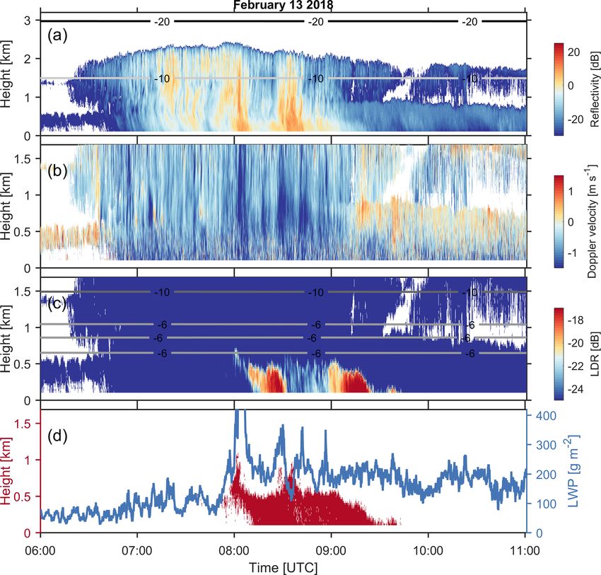
14672                       H. Li et al.: Two-year statistics of columnar-ice production in stratiform clouds over Hyytiälä

der et al., 2020). This dependence is more or less universal       Based on aircraft measurements from two field campaigns,
but can also be affected by other factors, such as the ge-         Korolev et al. (2020) concluded that the secondary ice pro-
ographic location, air-mass types and aerosol compositions         cess is highly associated with the presence of liquid droplets
(e.g., DeMott et al., 2010; Niemand et al., 2012; Wilson et al.,   and aged rimed ice in turbulent regions. Recently, Yang et al.
2015; DeMott et al., 2016; Petters and Wright, 2015; Mc-           (2020) found that the ice concentration in tropical maritime
Cluskey et al., 2018). In addition, it has been found that INP     stratiform clouds characterized by the top temperature above
concentrations at high latitudes are generally lower than at       −8 ◦ C is on the order of 10−1 –101 L−1 , which cannot be
mid-latitudes (e.g., DeMott et al., 2016; Wex et al., 2019).       fully explained by primary ice nucleation, H–M processes
Above −10 ◦ C, the typical concentrations of INPs are below        or droplet freezing. However, despite the advantage of offer-
10−1 L−1 and can be as low as 10−6 L−1 (Petters and Wright,        ing a direct way of interpreting ice microphysics, aircraft ob-
2015; Kanji et al., 2017). A number of studies, however,           servations are only available from a few measurement cam-
have reported that the ice number concentration in clouds          paigns and do not seem sufficient for a long-term assessment.
with the top temperature warmer than −10 ◦ C can exceed the           The polarimetric variables, such as differential reflectiv-
expected concentration of INPs by several orders of magni-         ity (Zdr ), specific differential phase measurements (Kdp )
tude (e.g., Mossop, 1985; Hobbs and Rangno, 1985; Rangno           and linear depolarization ratio (LDR), observed by dual-
and Hobbs, 2001). This discrepancy implies that numerical          polarization radars are sensitive to the shape of hydromete-
weather prediction models that rely solely on INP parame-          ors (Bringi and Chandrasekar, 2001) and allow the analy-
terizations cannot realistically represent ice number concen-      sis of ice particles with specific habits (e.g., Matrosov et al.,
trations in moderately to slightly supercooled clouds. As a        2001; Hogan et al., 2002; Tyynelä and Chandrasekar, 2014;
result, the inappropriate parameterization of ice production       Li et al., 2018). At temperatures of −10 to −2 ◦ C, the de-
may lead to biased estimates of surface shortwave radiation        positional growth of an ice crystal is stronger at the basal
budget (Young et al., 2019), among other things (e.g., Zhao        faces than at the prism faces. Hence, the formation of colum-
et al., 2021; Zhao and Liu, 2021).                                 nar ice is preferred (Lamb and Verlinde, 2011). This dis-
   Several mechanisms have been proposed to explain this           tinct habit can produce high Zdr and Kdp as observed by
discrepancy, such as the enhanced contact nucleation driven        dual-polarization weather radars (Hogan et al., 2002; Gi-
by the thermophoretic force during the evaporation of liquid       angrande et al., 2016; Sinclair et al., 2016). For vertically
drops (Beard, 1992; Hobbs and Rangno, 1985), pre-activated         pointing Ka- and W-band radars, ice columns usually pro-
INPs from evaporated ice particles nucleated above (Roberts        duce LDR values as high as −15 dB, which is distinctively
and Hallett, 1968; Fridlind et al., 2007) or secondary ice pro-    higher than that of most other ice particle types (Aydin and
duction (SIP) mechanisms (see recent reviews by Field et al.,      Walsh, 1999; Tyynelä et al., 2011). Oue et al. (2015), Li and
2017; Korolev and Leisner, 2020). The SIP has been stud-           Moisseev (2020), Luke et al. (2021), and Li et al. (2021)
ied by a number of laboratory experiments since the 1940s          have shown that this strong LDR signal at the slow falling
(e.g., Findeisen and Findeisen, 1943; Dye and Hobbs, 1966;         part of the radar Doppler spectrum can be used to identify
Wildeman et al., 2017). Hallett and Mossop (1974) found            columnar-ice crystals. In this study, this method is applied to
that numerous ice splinters can be generated when super-           long-term radar Doppler spectra observations for character-
cooled liquid drops larger than ∼ 25 µm are collected by           izing the production of columnar-ice particles in stratiform
large ice particles within the temperature range of −8 to          clouds. Similarly to Luke et al. (2021), we show that this
−3 ◦ C. This is referred to as the Hallett—Mossop (H–M)            phenomenon is not uncommon. By comparing radar-based
process, the most studied and most frequently implemented          retrievals of ice number concentrations to INP parameteriza-
SIP mechanism in numerical models (Field et al., 2017) de-         tions, one of which was derived from observations collected
spite more parameterizations for other SIP processes becom-        at our measurement site (Schneider et al., 2020), we show
ing available (e.g., Hoarau et al., 2018; Sullivan et al., 2018;   that the ice number concentrations tend to be 1–3 orders of
Zhao et al., 2021). The enhanced ice number concentration          magnitude higher than the expected INP concentration. This
can also be caused by the fragmentation of large supercooled       also supports the conclusions reached by Luke et al. (2021).
liquid droplets (e.g., Evans and Hutchinson, 1963; Scott and          The paper is organized as follows. Section 2 introduces the
Hobbs, 1977; Wildeman et al., 2017). It has been found that        data used in this study. The method for identifying columnar-
the secondary ice production efficiency is positively corre-       ice particles from radar Doppler spectra is illustrated in
lated with the size of liquid droplets (Lauber et al., 2018) and   Sect. 3. Statistical results are presented in Sect. 4. Section 5
is enhanced in moist environments (Keinert et al., 2020). At       compares the concentrations of columnar-ice particles and
temperatures higher than −3 ◦ C the fragmentation of drizzle       INPs in single-layer shallow clouds. Conclusions are given
is still active, as shown by field observations (Lauber et al.,    in Sect. 6.
2021). In addition, studies using optical sensors mounted on
aircrafts have reported the high concentration of ice columns
within the temperature range of −10 to −3 ◦ C (e.g., Koenig,
1963; Hobbs and Rangno, 1990; Rangno and Hobbs, 2001).

Atmos. Chem. Phys., 21, 14671–14686, 2021                                          https://doi.org/10.5194/acp-21-14671-2021
H. Li et al.: Two-year statistics of columnar-ice production in stratiform clouds over Hyytiälä                               14673

2     Data                                                         2.2    Model temperature and humidity profiles

2.1    Cloud radar observations                                    To obtain information on atmospheric state during the
                                                                   cloud observations, forecasts of the Deutscher Wetterdi-
The measurements used in this study were collected at Sta-         enst (DWD) operational global Icosahedral Nonhydrostatic
tion for Measuring Ecosystem – Atmosphere Relations II             (ICON) model (Zängl et al., 2015) were used. The micro-
(Hari and Kulmala, 2005; Petäjä et al., 2016) located in           physics scheme in ICON is inherited from the COSMO
Hyytiälä, southern Finland (61.845◦ N, 24.287◦ E; 150 m            model (Seifert, 2008). The ICON model output is provided
above mean sea level, a.m.s.l.). Since November 2017, a            over all Aerosol, Clouds and Trace Gases Research Infras-
94 GHz dual-polarization frequency-modulated continuous-           tructure (ACTRIS) cloud profiling stations (available at http:
wave Doppler cloud radar (Küchler et al., 2017) (HYytiälä          //cloudnet.fmi.fi/, last access: 30 July 2020). The model data
Doppler RAdar, HYDRA-W) has been operating at the sta-             have hourly temporal resolution with a horizontal resolution
tion. The radar is pointing vertically and measures radar sig-     of 13 km (Prill et al., 2019; Reinert et al., 2020). The height
nal spectral moments, LDR and dual-polarization Doppler            resolution decreases with the increase in altitude; for exam-
spectra; see Li and Moisseev (2020) for the example of the         ple, the height resolution is 0.16 km at an altitude of 1 km. Its
data. The LDR decoupling is about 30 dB, so the minimum            atmospheric products, such as temperature, relative humidity
observable LDR is about −30 dB. The radar operates us-             (RH) and pressure, over Hyytiälä were interpolated into the
ing three chirps that define range resolution, Doppler un-         temporal and spatial resolutions of HYDRA-W (CLU, 2021).
ambiguous velocity and spectral resolution at three range
intervals. Between 102 and 996 m, the range resolution
is 25.5 m, Doppler unambiguous velocity is 10.24 m s−1 ,           3     Methods
and the Doppler spectral resolution is 0.02 m s−1 . Between
996 and 3577 m, these values are 25.5 m, 5.12 m s−1 and            The mean Doppler velocity (MDV) of hydrometeors ob-
0.02 m s−1 , respectively. For ranges above 3577 m, they are       served by a vertically pointing radar is the combination of
34 m, 5.12 m s−1 and 0.02 m s−1 , respectively. In this study,     particle terminal fall velocities and the vertical component of
HYDRA-W observations recorded between February 2018                air motion. While Doppler velocity alone could be used to
and April 2020 were utilized (Moisseev, 2020).                     identify certain types of particles (Mosimann, 1995; Kneifel
   To remove noise from Doppler spectra observations, the          and Moisseev, 2020), there are associated limitations. These
spectral lines with the signal-to-noise ratio less than 5 dB       limitations include uncertainties in hydrometeor classifica-
were filtered out. Since both co-polar and cross-polar obser-      tion due to similarities of terminal fall velocities of dif-
vations were used, i.e., to compute spectral LDR, this fil-        ferent particles (Locatelli and Hobbs, 1974; Barthazy and
tering could result in complete removal of the cross-polar         Schefold, 2006; Li et al., 2020), the presence of a mixture of
signal, the power of which is typically 15–30 dB lower than        ice particle populations within the radar volume (Zawadzki
that of the co-polar signal (Bringi and Chandrasekar, 2001;        et al., 2001; Kalesse et al., 2019; Li and Moisseev, 2020)
Moisseev et al., 2002). In such cases, no LDR values were          and impact of air motion on the observed MDV (Protat and
computed.                                                          Williams, 2011). By using radar Doppler spectra instead of
   The antenna diameter of HYDRA-W is 0.5 m, which trans-          MDV, contributions from different particle populations can
lates into the Fraunhofer far-field distance of 157 m (Sekel-      be separated (e.g., Zawadzki et al., 2001; Kalesse et al.,
sky, 2002; Falconi et al., 2018) and antenna beam width of         2019; Radenz et al., 2019; Li and Moisseev, 2020; Luke
0.56◦ . Therefore, the lowest radar range bin, which is not        et al., 2021). In radar Doppler spectral power observations,
affected by the near-field effect, is 179 m (the fourth range      the presence of multiple populations of hydrometeors, such
bin). Data recorded at distance in the radar far-field were used   as the co-existence of supercooled liquid water and ice (e.g.,
in this study, therefore limiting the lowest altitude to 179 m     Zawadzki et al., 2001; Shupe et al., 2004; Luke et al., 2010;
where observations were taken.                                     Kalesse et al., 2016; Li and Moisseev, 2019), a mixture of
   In addition to the active remote sensing system, HYDRA-         different ice types (e.g., Zawadzki et al., 2001; Kalesse et
W is capable of estimating the liquid water path (LWP) by us-      al., 2019; Radenz et al., 2019; Li and Moisseev, 2020), could
ing the 89 GHz passive microwave channel observations. The         manifest as multiple spectral peaks. Even in such cases, how-
brightness temperature at this band is regularly calibrated        ever, classification of these particles can be ambiguous.
using liquid nitrogen. The site-specific relation between the         To further improve the hydrometeor identification, dual-
measured 89 GHz brightness temperature and LWP was de-             polarization radar observations can be used. For slant mea-
rived by the radar manufacturer using radio-sounding and re-       surements the spectral differential reflectivity has been found
analysis data.                                                     to be useful (Spek et al., 2008). Because hydrometeors typi-
                                                                   cally do not have a preferred azimuth orientation, the differ-
                                                                   ential reflectivity is not very useful for the classification pur-
                                                                   poses at vertical incidence. Nonetheless, LDR can be used to

https://doi.org/10.5194/acp-21-14671-2021                                          Atmos. Chem. Phys., 21, 14671–14686, 2021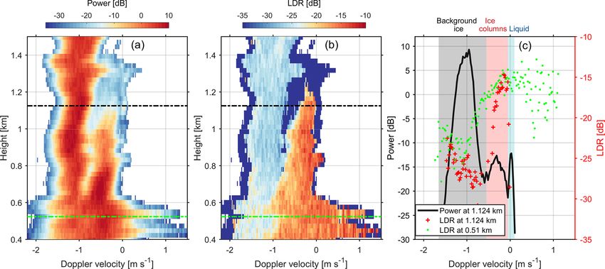
14674                        H. Li et al.: Two-year statistics of columnar-ice production in stratiform clouds over Hyytiälä

identify prolate particles (Myagkov et al., 2016a, b), such as       4     Results
ice columns (Oue et al., 2015). At an elevation angle of 90◦ ,
columnar-ice particles can produce LDR signals as high as            By utilizing HYDRA-W Doppler spectral observations
−16 to −13 dB (Oue et al., 2015), while other ice particles          recorded between February 2018 and April 2020, statistics of
may produce values smaller than −20 dB (e.g., Tyynelä et al.,        environmental conditions associated with columnar-ice pro-
2011). Furthermore, given the relatively small fall veloci-          duction were derived. All detected cloud cases within the
ties of newly produced columns, in regions where they co-            temperature range of −10 to 0 ◦ C were analyzed. From the
exist with other ice particles they usually populate the slow-       selected events the cases where significant inversion was
falling part of the Doppler spectrum. Therefore, the slow-           detected, which could cause melting (e.g., Kumjian et al.,
falling part characterized by high spectral LDR (∼ −15 dB)           2020), were excluded. Given the data selection criteria, no
in the Doppler spectrum indicates the presence of columnar-          rainfall or summer cloud cases were analyzed. This was done
ice particles (Oue et al., 2015; Radenz et al., 2019).               to avoid potential problems due to radar signal attenuation
   Figure 1 shows an example of observed spectral power              in rain and melting layer (Li and Moisseev, 2019). In to-
and LDR. Two distinct populations of ice particles can be            tal, 175 d of observations satisfying the data selection criteria
clearly identified from Fig. 1a, and the slower-falling one          were identified and analyzed.
corresponds to ice columns as indicated by the high spec-
tral LDR (Fig. 1b). The observed spectral power and LDR at           4.1    Temperature and RH conditions in
1.124 km (black dot dashed lines) are shown in Fig. 1c. Three               columnar-ice-producing regions
distinct peaks can be identified from the spectral power, and
the slower-falling ice columns are well characterized by the         Formation and growth of ice particles require favorable en-
spectral LDR exceeding −18 dB. In contrast, the spectral             vironmental conditions. These conditions were assessed by
LDR of faster-falling ice is around −25 dB, which mainly de-         using ICON forecasts, which supplemented the radar ob-
pends on the cross-coupling between the polarization chan-           servations. Here, we define Hcolumn_top as the highest level
nels (Moisseev et al., 2002) and can be much higher than the         where ice columns are detected and Tcolumn_top as the tem-
LDR signal of larger aggregates (Tyynelä et al., 2011). In-          perature at this height. As shown in Fig. 2a, Tcolumn_top val-
terestingly, supercooled liquid water also seems present, as         ues are mostly between −8 and −3 ◦ C, with the highest fre-
indicated by the well-defined spectral peak at around 0 m s−1        quency at around −5 ◦ C and a median value of −4.7 ◦ C.
(Zawadzki et al., 2001; Shupe et al., 2004; Luke et al., 2010;       These values are within the growth region of ice columns
Kalesse et al., 2016; Li and Moisseev, 2019). It appears that        (Lamb and Verlinde, 2011). Such temperature distribution
this liquid layer extends from ∼ 0.9 to ∼ 1.3 km (Fig. 1a).          also bears a good resemblance to the results obtained from
The potential mechanisms of producing these ice columns              the early rime-splintering laboratory experiment (Hallett and
will be discussed in more detail in the following sections.          Mossop, 1974) and a recent statistical study (Luke et al.,
   Given the spectral characteristics of ice columns as dis-         2021). The statistics of humidity relative to ice (RHice ) and
cussed above, the following criteria were set to identify ice        water (RHliquid ) at Hcolumn_top are shown in Fig. 2b. The me-
columns in clouds.                                                   dian values of RHice and RHliquid are 102.6 % and 98.3 %,
                                                                     respectively, indicating the supply of water vapor is suffi-
  – Within the slowest 1 m s−1 of the Doppler spectrum, at           cient for growth of ice particles. This finding is, however, not
    least three spectral bins exceed the LDR of −18 dB.              surprising, since the method detects ice columns, and they
  – The temperature of the radar range bin is between −10            are growing in this temperature regime. However, the val-
    and 0 ◦ C.                                                       ues of RHliquid and RHice should be interpreted with caution.
                                                                     ICON applies a liquid saturation adjustment, limiting the liq-
   The observed radar Doppler spectrum is not only depen-            uid supersaturation to saturation. RHliquid values exceeding
dent on the scattering properties of hydrometeors in the radar       100 % are attributed to numerical artifacts. RHice was calcu-
volume, but is also affected by the turbulent broadening (Kol-       lated based on the forecasted temperature, pressure as well as
lias et al., 2011; Tridon and Battaglia, 2015). For example,         RHliquid and therefore can be affected by numerical artifacts
the air at around 0.51 km seems rather turbulent, as indicated       as well. Given the uncertainty of ICON forecasts, we regard
by the spectral power (green dashed line in Fig. 1a). How-           the presented statistics in Fig. 2 as a “sanity” check for our
ever, it appears that this issue does not significantly affect the   method.
results of columnar-ice detection. The noisy spectral LDR               It should be noted that although ice columns can be de-
values (green dots in Fig. 1c) between 0.3 and 1 m s−1 are           tected by our method, Hcolumn_top may be lower than the
attributed to the low signal-to-noise ratio. Such weak impact        height where ice crystals are generated. There are two poten-
on spectral LDR due to turbulence may be explained by the            tial reasons for this. Firstly, the newly formed ice particles
distinctively high LDR values of ice columns, which contrast         may be less non-spherical (Korolev et al., 2020; Luke et al.,
with much weaker LDR signals of ice aggregates (Tyynelä              2021), and in this case they will have LDR values which are
et al., 2011).                                                       much smaller than our detection threshold. Secondly, at early

Atmos. Chem. Phys., 21, 14671–14686, 2021                                            https://doi.org/10.5194/acp-21-14671-2021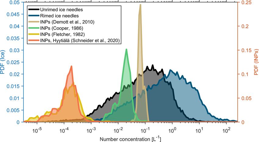
H. Li et al.: Two-year statistics of columnar-ice production in stratiform clouds over Hyytiälä                                      14675

Figure 1. HYDRA-W Doppler spectral (a) power and (b) LDR at 2 February 2018 07:56:38 UTC. (c) Spectral power (black line) and LDR
(red crosses) at 1.124 km as marked by the black dot dashed lines in (a) and (b) and LDR (green dots) at 0.51 km as marked by the green dot
dashed lines in (a) and (b). The gray, red and blue shaded areas in (c) indicate background ice falling from above, newly formed ice columns
and supercooled liquid, respectively, at 1.124 km. Negative velocity indicates downward motion.

                                                                        Figure 3. Duration of cloud observations (bars) and occurrence of
Figure 2. Statistics of (a) temperature (Tcolumn_top ) and (b) rela-
                                                                        columnar-ice-producing clouds (red dotted curve) over Hyytiälä as
tive humidity (RH) at Hcolumn_top for all identified columnar-ice-
                                                                        a function of cloud top temperature (CTT). The results were calcu-
producing cases. Hcolumn_top : the highest level where ice columns
                                                                        lated based on the data collected from February 2018 to April 2020.
are detected.

stages of growth the radar signal of ice crystals is rather weak        particles falling from upper cloud layers, i.e., by SIP, the lo-
and does not allow accurate detection and identification of             cation where ice columns are forming, with respect to the
columns (Luke et al., 2021). However, the altitude difference           cloud top, should be identified. Finally, the importance of the
between Hcolumn_top and the actual height where columns are             columnar-ice production for surface precipitation should also
generated is expected to be small and not significantly affect          be assessed.
our results.                                                               To identify such conditions, cloud top temperature (CTT),
                                                                        defined as the temperature of the highest detected radar re-
4.2   Properties of columnar-ice-producing clouds                       turn for a given measurement time, is used. Because there
                                                                        are cases where several cloud layers are observed and there
There are a number of questions that are associated with                are gaps between these layers, typically the top of the lowest
formation of ice crystals in clouds at these relatively warm            one is used. However, particles forming in the upper clouds,
temperatures. Above −10 ◦ C, the number concentration of                while not detected by the radar, may seed lower cloud layers
INPs is expected to be small and rather uncertain (DeMott               and therefore modify their properties (Vassel et al., 2019).
et al., 2010; Kanji et al., 2017). Therefore, it is important to        To limit the impact of such conditions on our analysis, fol-
know how often and under which conditions these ice crys-               lowing Seifert et al. (2009) we have used a radar echo gap
tals form. Because ice formation could be facilitated by ice            of 2 km as the threshold, which defines whether the layers

https://doi.org/10.5194/acp-21-14671-2021                                               Atmos. Chem. Phys., 21, 14671–14686, 2021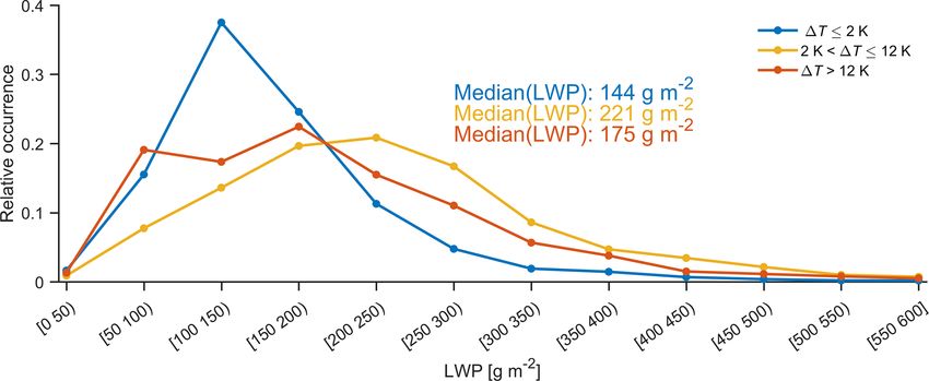
14676                         H. Li et al.: Two-year statistics of columnar-ice production in stratiform clouds over Hyytiälä

Figure 4. Comparison of liquid water path (LWP) for clouds with         Figure 5. The same as Fig. 4 but for W-band radar reflectivity at the
and without columnar-ice production. A cloud sample was identi-         fourth range bin (179 m above the surface).
fied if the cloud base was within the temperature range of −10 to
0 ◦ C. The box plots represent the median (horizontal strip) and 5 %–
95 % quantile (whisker) ranges of the distribution.
                                                                        roles in formation of ice columns. Given the mixed-phase
                                                                        cloud conditions, the observed columns are most probably
                                                                        ice needles.
are connected. Recently, Proske et al. (2020) suggested that               Formation of ice crystals is an efficient precipitation pro-
the threshold of 2 km may overestimate the cases of cloud               cess (Lamb and Verlinde, 2011). To evaluate the impact of
seeding. For this reason, we have also tried the threshold of           columnar-ice production on precipitation, the radar equiva-
0.5 km to determine the cloud top, but we did not see signifi-          lent reflectivity factor is used as the proxy for the precipi-
cant changes in the results.                                            tation intensity. For clouds where the radar echo extends to
   The statistics of the recorded cloud top temperatures are            the ground, reflectivity values at the fourth radar gate, 179 m
presented in Fig. 3. The figure (left) shows durations of de-           above ground level (a.g.l.), were used. As shown in Fig. 5, the
tected cloud samples within the temperature of −10 to 0 ◦ C             reflectivity increases with decreasing CTT. This is due to the
for a given CTT range as recorded during the observation                link between the cloud thickness and precipitation intensity.
period. Because of the focus on cold cloud cases, where the             The columnar-ice production tends to increase the precipi-
temperature in an atmospheric column does not exceed 0 ◦ C,             tation intensity. This effect is more pronounced for warmer
the observed cloud cases were recorded between October                  clouds, where CTT is −12 ◦ C or warmer. In warmer clouds
and April. The observations show that low-level clouds, i.e.,           the precipitation intensity can be enhanced by as much as 10-
clouds with warmer CTT, are relatively more frequent. This              fold. The factor of 10 increase in precipitation rate appears
resembles the cloud occurrence statistics of, e.g., Hagihara            from the 10 dB increase in reflectivity (Falconi et al., 2018).
et al. (2010) and Shupe et al. (2011). It appears that deeper           As will be discussed in the next section, warmer clouds tend
clouds, i.e., where CTT is below −12 ◦ C, are more conducive            to be single-layer clouds, where the crystal formation is more
to columnar-ice production. In these cases the frequency of             directly linked to precipitation formation. Colder clouds are
columnar-ice occurrence is about 25 %–33 %. For warmer                  prone to consist of the multiple cloud layers where precipi-
clouds the frequency is lower and is around 5 %–13 %. The               tation processes are affected by multiple processes, such as
average occurrence is 15 %. Interestingly, our results are              riming, aggregation, and sublimation, at various levels (e.g.,
comparable with a recent study by Luke et al. (2021), who               Houze and Medina, 2005; Verlinde et al., 2013; Moisseev
found that the occurrence of columnar ice over an Arctic site           et al., 2015)
is between 10 % and 25 % depending on the temperature.
   As shown in Fig. 2b, the majority of columnar-ice produc-
tion cases took place in areas around liquid saturation. Al-            4.3   Columnar-ice production in single-layer and
though direct observations of liquid were not available, the                  multilayered clouds
measurements collected by the 89 GHz passive channel in
HYDRA-W allows estimation of LWP. The LWP values for                    For all detected columnar-ice-producing cases, the distribu-
the cloud cases are shown in Fig. 4. The observations show              tion of CTT was analyzed. As shown in Fig. 6a, ice columns
a significant amount of supercooled liquid water present in             can form in clouds with a wide range of CTT. The major-
the atmospheric column. The cloud cases where ice columns               ity of cases fall in the CTT range of −20 to 0 ◦ C, with two
were detected tend to have larger LWP values, especially                peaks at around −15 and −5 ◦ C, respectively. The peak at
where CTT values were smaller than −8 ◦ C. This potentially             around −15 agrees rather well with the high occurrence of
indicates that supercooled liquid droplets may play important           ice columns in clouds, with a CTT of −20 to −12 ◦ C (Fig. 3).

Atmos. Chem. Phys., 21, 14671–14686, 2021                                                https://doi.org/10.5194/acp-21-14671-2021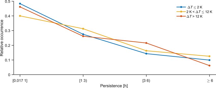
H. Li et al.: Two-year statistics of columnar-ice production in stratiform clouds over Hyytiälä 14677
Figure 6. Relative occurrence of (a) CTT and (b) 1T for columnar-
ice production cases. 1T = Tcolumn_top − CTT.
Because processes responsible for the formation of ice par-
ticles in single-layer and multilayered clouds may be dif-
ferent, the classification of the cloud cases was performed.
Using CTT and Tcolumn_top , we define 1T as the tempera-
ture difference between them. The larger 1T is, the lower Figure 7. The columnar-ice-producing event on 4 November 2019.
the inside of the observed cloud system where the columns HYDRA-W observations of (a) equivalent reflectivity factor,
are formed. The relative occurrence of 1T also shows two (b) mean Doppler velocity, where negative velocity indicates down-
peaks as presented in Fig. 6b. Specifically, one peak is close ward motion, and (c) LDR. Panel (d) presents the (left axis) detected
to 1T = 0 K, indicating that ice columns are generated close columnar-ice region and (right axis) LWP observed by HYDRA-W.
to the cloud top. The second 1T peak is around 10 K. The lines in (c) are isotherms produced by ICON.
Given the distinct distribution of 1T , we have grouped the
recorded clouds into the following three categories.
detail later. Regarding the SIP, the H–M process does not
– Type 1: 1T ≤ 2 K – columnar-ice production at cloud
seem to be active since it requires falling ice particles serv-
top
ing as rimers to produce ice splinters (Hallett and Mossop,
– Type 2: 2 K < 1T ≤ 12 K – multilayered cloud 1974).
As shown in Fig. 6, around 22 % of columnar-ice produc-
– Type 3: 12 K < 1T – multilayered cloud tion cases are attributed to single-layer shallow clouds. Bühl
Representative events of the above cloud types are pre- et al. (2016) also observed the prevalence of high LDR values
sented below. for mixed-phase clouds, with a CTT of −5 ◦ C. They specu-
lated that these particles are formed mainly by primary ice
4.3.1 Columnar-ice production at cloud top: 1T ≤ 2 K nucleation instead of the SIP. Recently, Yang et al. (2020) re-
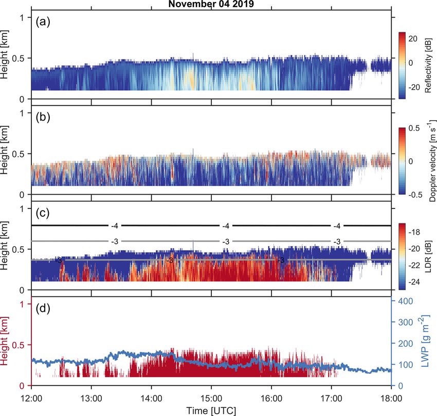
ported a similar event of shallow stratiform clouds over the
This type of cloud is usually single layer, and ice columns tropical ocean and found that neither INPs nor known SIP
are generated close to the cloud top. Figure 7 presents such mechanisms can fully explain the strong production of ice
an event on 4 November 2019. The precipitation intensity particles in such clouds, with top temperatures warmer than
is relatively light, with the CTT at around −3 ◦ C. The W- −8 ◦ C. In this study, we find that such clouds also frequently
band reflectivity close to the surface increases to around occur over Hyytiälä, and more detailed analysis will be pre-
0 dB between 14:00 and 16:00 UTC. This region coincides sented in Sect. 5.
with the enhanced LDR observations, which reaches values
as high as −15 dB. Such high LDR values indicate that the 4.3.2 Columnar-ice production in multilayered clouds:
dominant ice particle type during this period is columns. As 2 K < 1T ≤ 12 K
shown in Fig. 7b, the cloud top is turbulent and seems to be
capped by an inversion layer (Fig. 7c). The observed LWP The event that took place on 13 February 2018 is repre-
ranges between 80 and 150 g m−2 . This cloud with relatively sentative of the second cloud type, as defined by 1T . As
low reflectivity persisted over Hyytiälä for about 1 d (not shown in Fig. 8a, the precipitation intensity during this event
shown). Given the warm cloud top, the primary ice nucle- is higher than during the discussed single-layer shallow cloud
ation may not fully explain the significant columnar-ice pro- case. The cloud top temperature of the upper cloud layer
duction (DeMott et al., 2010), as will be discussed in more is about −15 to −12 ◦ C. Before 08:00 UTC, the observed
https://doi.org/10.5194/acp-21-14671-2021 Atmos. Chem. Phys., 21, 14671–14686, 202114678 H. Li et al.: Two-year statistics of columnar-ice production in stratiform clouds over Hyytiälä
Figure 8. The columnar-ice-producing event recorded on 13 Febru- Figure 9. Same as Fig. 8 but for the columnar-ice-producing event
ary 2018. HYDRA-W observations of (a) equivalent reflectivity observed on 2 February 2018. A zoom-in view on the wave signa-
factor, (b) mean Doppler velocity, where negative velocity indi- tures between 05:30 and 07:00 UTC is presented in (b).
cates downward motion, and (c) LDR. Panel (d) presents the (left
axis) detected columnar-ice region and (right axis) LWP observed
by HYDRA-W. The lines in (a) and (c) are isotherms produced by
ICON. Note that the y-axis scale in (a) is different from that in (b), 4.3.3 Deep multilayered clouds: 1T > 12 K
(c) and (d).
The third cloud type is not very different from the sec-
ond one and represents the tail of the observed 1T distri-
LWP is close to 100 g m−2 , and the mean Doppler velocity bution as shown in Fig. 6. This type of cloud system is a
at around 0.8 km is relatively small (∼ 1 m s−1 ), which indi- deeper precipitating system with a CTT of −60 to −40 ◦ C;
cates that particles are unrimed or very lightly rimed. From see Fig. 9 for an example. The presented case took place
08:00 to 09:30 UTC, the falling snowflakes seem to be heav- on 2 February 2018. There are several features that are
ily rimed, as revealed by a rather high LWP (from 200 to over worthwhile pointing out. The mean Doppler velocity obser-
400 g m−2 ) and mean Doppler velocity measurements (1.2– vations exhibit signatures of atmospheric waves. Between
1.8 m s−1 ) (Kneifel and Moisseev, 2020). The high LWP pe- 05:00 and 06:00 UTC such waves can be observed at around
riod coincides with the region of ice columns (Fig. 8d). Dur- 1 km altitude. At the later time, the wave signatures appear
ing this period, the observed LDR values are enhanced but at 0.5 km a.g.l. The strongest velocity variation, observed
still relatively small. This is due to masking of the needle around 06:00 UTC, seems to coincide with the LWP peak.
LDR signal by larger snowflakes. At the same time as the waves are observed, signatures of
This type of cloud frequently occurs over Hyytiälä (Figs. 3 columnar-ice production are also detected, pointing to a pos-
and 6). Although sounding measurements were absent, this sible connection between the two.
cloud type seems to very similar to the one reported by West- Deep precipitating clouds usually have a large number
brook and Illingworth (2013), namely, a layer of supercooled of ice crystals formed at the cloud top. Given the large
liquid water with the top temperature of around −15 ◦ C seed- ice flux, manifested by the higher radar reflectivity values,
ing low-level stratus clouds in the boundary layer. In this in this precipitation system, it is difficult for supercooled
event, the presence of supercooled liquid water may not be liquid droplets to survive. The supercooled water droplets
directly determined; however, the enhanced LWP values are can be rapidly depleted through the Wegener—Bergeron—
indicative of the vigorously supercooled liquid water genera- Findeisen (WBF) process (Lamb and Verlinde, 2011; Ko-
tion. In addition, the falling ice particles between 08:00 UTC rolev et al., 2017) as well as riming (Fukuta and Takahashi,
and 09:30 UTC seem to be heavily rimed, as evident from 1999). Nevertheless, the atmospheric waves could generate
mean Doppler velocity (Kneifel and Moisseev, 2020). The conditions needed for forming and maintaining the presence
combination of the presence of supercooled liquid water and of supercooled liquid water droplets (Korolev, 1995; Korolev
riming indicates that the H–M process could be taking place and Field, 2008; Majewski and French, 2020). Recently, Li
and could be responsible for the columnar-ice production. et al. (2021) provided radar observational evidence showing
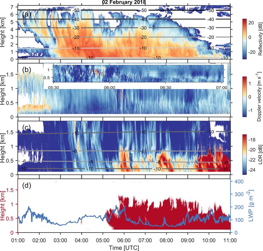
Atmos. Chem. Phys., 21, 14671–14686, 2021 https://doi.org/10.5194/acp-21-14671-2021H. Li et al.: Two-year statistics of columnar-ice production in stratiform clouds over Hyytiälä 14679
Figure 10. Relative occurrence of the persistence of columnar- Figure 11. Relative occurrence of LWP for all columnar-ice-
ice-producing events from February 2018 to April 2020. 1T = producing events. LWP: liquid water path. 1T = Tcolumn_top −
Tcolumn_top − CTT. CTT.
that the Kelvin–Helmholtz instability is favorable for super- columnar-ice-producing clouds have higher LWP values
cooled drizzle and secondary ice production. In such cases, (Fig. 4). For different columnar-ice-producing cloud types,
ice needles may be generated by the H–M process (Hogan the observed LWP values seem to be somewhat different.
et al., 2002; Houser and Bluestein, 2011) or freezing breakup Figure 11 shows LWP occurrence for these three cloud types.
(Luke et al., 2021; Li et al., 2021). In general, their distributions are similar, while identifiable
differences still exist. The median value of LWP for single-
4.4 Characteristics of different layer clouds is the lowest, and the second type of cloud has
columnar-ice-producing cloud types the highest LWP. Interestingly, while both the second and
third types of clouds are multilayered, the LWP of the sec-
As discussed above, we have identified three types of cloud ond type is detectably higher than for the third one. Com-
systems where columnar-ice particles form. To better under- paring Figs. 8 and 9, we find that the radar reflectivity above
stand how columnar-ice production is related to cloud prop- the columnar-ice layer is generally higher in the third cloud
erties, persistence of columnar ice in these clouds and the type than the second one. The INP concentrations in clouds
amount of LWP were considered for further analysis. with a cold top are expected to be higher than for warmer
clouds, and hence more falling ice particles are expected for
4.4.1 Persistence of columnar-ice crystals
deep precipitating clouds. Therefore, we speculate that one
As was demonstrated by the case studies, the columnar- of the reasons for the difference in LWP may be the ice num-
ice production may persist over several hours, and therefore ber concentration, which is related to the consumption of the
these particles may play a major role in determining cloud liquid water via the WBF process (Lamb and Verlinde, 2011)
properties. To document this, we have derived statistics of and riming (Fukuta and Takahashi, 1999).
the columnar-ice production persistence for each cloud case.
This was done by computing the duration of a continuous
columnar-ice production event. Since in some cases, for ex- 5 Potential role of SIP in columnar-ice production in
ample, in the presented shallow single-layer clouds (Fig. 7) single-layer shallow clouds
formation of columns may be intermittent in nature (as can
also be seen in Luke et al., 2021), similar to Shupe et al. Given the rather frequent formation of ice crystals at temper-
(2011), gaps of less than 30 min were accepted. In addition, atures warmer than −10 ◦ C, where expected INP concentra-
cases persisting for less than 1 min were removed. As shown tions are low, it is important to investigate a potential role of
in Fig. 10, 40 %–50 % of columnar-ice-producing events per- SIP. In multilayered clouds, identified here as cloud types II
sist for less than 1 h. However, there is a significant fraction and III, it has been found that the ice formation can be en-
that could last for more than 3 or even 6 h. This hints that the hanced by the H–M process (e.g., Grazioli et al., 2015; Gi-
production of ice columns plays an important role in defining angrande et al., 2016; Sinclair et al., 2016; Keppas et al.,
cloud properties and should be included while considering 2017; Sullivan et al., 2018; Gehring et al., 2020), among
radiative or precipitation properties of such clouds (see, for other mechanisms (Korolev and Leisner, 2020). In single-
example, Fig. 9). layer clouds the mechanisms for ice multiplication are less
established. However, recent studies by Lauber et al. (2018)
4.4.2 LWP and Keinert et al. (2020) have shown that freezing fragmenta-
tion may play such a role. To study whether these columnar-
Presence of liquid water droplets may be a necessary ice particles can be attributed to the SIP, the estimated ice
condition for the formation of the observed ice columns. number concentrations are compared to the expected INP
Compared to clouds where no ice columns were detected, concentrations. If the derived ice number concentrations ex-
https://doi.org/10.5194/acp-21-14671-2021 Atmos. Chem. Phys., 21, 14671–14686, 202114680 H. Li et al.: Two-year statistics of columnar-ice production in stratiform clouds over Hyytiälä
ceed these of INPs, we can conclude that the SIP is poten- radar reflectivity measured close to the ground, in the fourth
tially active in such clouds. The concentration of INPs was radar gate, 329 m a.m.s.l. or 179 m a.g.l., is used in this re-
computed by using CTT in the following different parame- trieval. The selection of the reflectivity measured close to the
terizations. ground helps to limit potential attenuation problems as well.
Using IWC, the number concentration of ice needles, Nneedle ,
– Fletcher (1962) parameterization based on INP mea- can be estimated as follows (Li et al., 2021):
surements obtained below −10 ◦ C.
IWC
– Cooper (1986) parameterization which is not directly Nneedle = 3
(L−1 ), (2)
10 mneedle
derived from INP measurements but the observed ice
number concentrations when the impact of SIP is min- where mneedle is the mass of a characteristic ice needle. The
imized. The temperature of measurements is between introduced uncertainty at this step depends on the defini-
−30 and −5 ◦ C. tion of the characteristic needle. Here, we use mean Doppler
velocity (MDV) and the velocity–mass relation to estimate
– DeMott et al. (2010) parameterization based on INP mneedle . Since MDV is reflectivity weighted, mneedle would
measurements from nine sites between −35 and be mainly determined by larger ice particles, and therefore
−9 ◦ C. In our study we have used the average INP the resulting Nneedle is underestimated. For the purpose of
concentration–temperature relation presented in De- this study, this underestimation is not a major issue, because
Mott et al. (2010). we want to test whether the observed Nneedle exceeds ex-
pected INP concentrations.
– Schneider et al. (2020) parameterization derived from
There are a number of reported ice needle properties. To
the INP measurements obtained at Hyytiälä. The tem-
take into account potential differences in ice needle prop-
perature range is −20 to −8 ◦ C. Also from this study,
erties, two relations linking velocity and mass by Kajikawa
the average INP concentration–temperature relation was
(1976) for rimed needles and Heymsfield (1972) for unrimed
used.
needles were used. For rimed ice needles, the relation be-
As was previously discussed, the INP parameterizations tween terminal fall velocity and mass was derived by Ka-
differ significantly at these temperatures (−10 to 0 ◦ C), as jikawa (1976) and can be written as
shown in Fig. 12. It should be noted that not all parameteri-
vneedle, rimed = 1.55(103 mneedle, rimed )0.271
zations were derived using observations at these cloud tem- 0.4
peratures, and some of them were extrapolated beyond their ρ(z)
· (m s−1 ), (3)
validity range. The most interesting comparison is to Schnei- ρ(1024 m)
der et al. (2020), which is based on observations at Hyytiälä
collected during 2018, so their observation period at least where mneedle, rimed is the mass of rimed ice needles, and the
h i0.4
partially overlaps with ours. It should also be pointed out that ρ(z)
term ρ(1024 m) accounts for the change in air density ρ
INP observations were carried out at the ground, where INP at a given height z (Heymsfield et al., 2007). In our study z
concentrations are typically higher. is 329 m, and in Kajikawa (1976) the altitude where needles
Radar-based retrieval of particle number concentration is were observed is 1024 m. For unrimed needles, Heymsfield
rather uncertain. Because of this uncertainty, the derived (1972) derived a relation linking terminal fall velocity and
number concentrations should be treated as our best esti- needle length, L. The terminal velocity of unrimed needles
mates of the order of magnitude of the ice column number at a given height can be estimated as follows (Heymsfield,
concentration. As shown in Fig. 4, the observed LWP for 1972):
columnar-ice-producing clouds is significantly higher than
those without ice columns. Hence, pristine ice crystals are vneedle, unrimed = 0.0006 + 0.2796L − 0.0497L2
anticipated to grow in mixed-phase conditions, and ice nee- ρ(z) 0.4
dles rather than solid columns are expected to form (Lamb + 0.0041L3 (m s−1 ). (4)
and Verlinde, 2011). This limits the parameter space, where ρ(0 m)
we need to search for microphysical properties of ice parti- The needle can be modeled as a cylinder, the mass of
cles to constrain our retrieval. The retrieval is based on esti- which is
mating ice water content from radar observations, following
10−3 π
Hogan et al. (2006), as mneedle, unrimed = ρice LD 2 (g), (5)
4
IWC = 100.00058ZT +0.0923Z−0.00706T −0.992 (g m−3 ), (1) where ρice and D denote density of unrimed needles and the
minor axis, respectively. Their parameterizations have been
where Z is the W-band radar reflectivity and T is the air given by Heymsfield (1972):
temperature. Because in a single-layer shallow cloud (1T ≤
2 ◦ C) ice needles are the predominant precipitation particles, ρice = 0.6L−0.117 (g cm−3 ) (6)
Atmos. Chem. Phys., 21, 14671–14686, 2021 https://doi.org/10.5194/acp-21-14671-2021H. Li et al.: Two-year statistics of columnar-ice production in stratiform clouds over Hyytiälä 14681
analysis was performed on shallow single-layer clouds, this
discrepancy may not be explained by the H–M process (Hal-
lett and Mossop, 1974) since no rimers are falling from upper
clouds. So it appears that other, less studied, SIP mechanisms
may play an important role in amplifying ice number con-
centrations in such shallow clouds. This conclusion is in line
with a number of other studies. For example, Knight (2012)
found that the SIP may take place at −5 ◦ C in the absence of
rimers, for which the cause is still under investigation. Re-
cently, a similar finding was reported for stratiform clouds
over the tropical ocean by Yang et al. (2020). They have
speculated that droplet collisional freezing (Hobbs, 1965;
Figure 12. Probability density function (PDF) of estimated colum- Alkezweeny, 1969) and pre-activated INPs (Roberts and Hal-
nar ice (left) and INP (right) concentrations in shallow single-layer lett, 1968; Mossop, 1970) could be responsible for this dis-
clouds. INPs: ice-nucleating particles. crepancy. Recent laboratory studies (Lauber et al., 2018;
Keinert et al., 2020) have shown that freezing breakup may
be a source of secondary ice particles. Luke et al. (2021) have
and also suggested that freezing breakup may be more efficient
D = 0.1973L0.414 (mm). (7) than the H–M process in nature.
Applying the power law fit to mneedle, unrimed and
vneedle, unrimed values when L ∈ [0.03, 5] (mm) yields 6 Conclusions
vneedle, unrimed = 1.09(103 mneedle, unrimed )0.377 This study documents formation of ice particles in clouds
ρ(z) 0.4
at the temperatures of −10 ◦ C or warmer. The analysis
· (m s−1 ). (8) was performed using W-band cloud radar observations col-
ρ(0 m)
lected at the University of Helsinki Hyytiälä station start-
The observed MDV is affected by vertical air motion. ing from February 2018 through April 2020. The columnar-
To at least partially mitigate this issue, the observed MDV ice particles were identified using measurements of spectral
is averaged over 20 min (Protat and Williams, 2011; Mosi- LDR. It was found that columnar-ice formation is relatively
mann, 1995; Kneifel and Moisseev, 2020; Silber et al., 2020). frequent in clouds at temperatures of −10 ◦ C or warmer.
While this step reduces the impact of air motion by averaging The occurrence frequency of columnar-ice particles is 5 %–
Doppler velocity over updrafts and downdrafts, the residual 13 % in clouds, with top temperatures exceeding −12 ◦ C. In
air motion is expected to widen the retrieved distribution of colder clouds, this percentage can be as high as 33 %. The
Nneedle . columnar-ice-producing clouds tend to have a higher LWP,
The derived number concentrations of ice particles are potentially indicating that supercooled water droplets are im-
compared to expected INP concentrations (Fig. 12). The re- portant for formation of the observed ice particles. It was also
sults show that the estimated ice number concentrations for observed that columnar-ice production seems to have a sig-
rimed needles (Kajikawa, 1976) are generally larger than nificant impact on the surface precipitation. This effect is es-
that of unrimed needles (Heymsfield, 1972). Regardless of pecially important for warmer clouds.
the difference between rimed and unrimed needles and the Using the temperature difference, 1T , between the alti-
INP parameterization used, there seems to be a large frac- tudes where columns are first detected and cloud top, the
tion of cases where INP concentrations are not sufficient to columnar-ice-producing clouds were subdivided into three
explain observed Nneedle . Our results are similar to the con- categories. The first category, where 1T is less than or equal
clusion reached by Luke et al. (2021), who used a different to 2 K, represents shallow single-layer clouds. In these clouds
approach for establishing the range of ice crystal concentra- ice particles are forming at or close to the cloud top. The
tion from radar observations. As shown in Fig. 12, the major- other two categories, where 2 K < 1T ≤ 12 K and 1T >
ity of Nneedle values fall in the range of 10−2 –101 L−1 , which 12 K, represent deeper multilayered clouds. In multilayered
is similar to aircraft measurements obtained in tropical strat- cloud systems, columnar-ice crystals are forming in the lower
iform clouds (Yang et al., 2020). cloud layer seeded by ice particles falling from upper cloud
The significant discrepancy between INP concentrations levels. It was observed that 40 %–50 % of columnar-ice pro-
estimated from INP parameterizations and retrieved ice num- duction cases persist for 1 h or less, while in some cases
ber concentrations indicates that primary ice nucleation does they can persist for over 6 h. The distributions of LWP val-
not seem to be the only mechanism responsible for the for- ues for the three types of columnar-ice-producing clouds
mation of ice particles in these shallow clouds. Because the are somewhat different. The median LWP value is largest
https://doi.org/10.5194/acp-21-14671-2021 Atmos. Chem. Phys., 21, 14671–14686, 202114682 H. Li et al.: Two-year statistics of columnar-ice production in stratiform clouds over Hyytiälä
(221 g m−2 ) in clouds where 2 K < 1T ≤ 12 K. Such high We thank the European Research Infrastructure for the observa-
LWPs could favor riming and cause the Hallet–Mossop pro- tion of ACTRIS for providing the DWD ICON (Global) model data,
cess. To draw a definite conclusion, however, a more thor- which were produced by the DWD and the Finnish Meteorological
ough study, where locations of supercooled liquid layers are Institute and are available for download from https://cloudnet.fmi.fi/
identified, is needed. For the single-layer shallow clouds, (last access: 1 October 2021). ACTRIS has received funding from
the European Union’s Horizon 2020 research and innovation pro-
number concentrations of ice columns were derived from the
gram under grant agreement no. 654109.
radar observations. It was observed that the concentration of
ice particles exceeds the expected concentration of INPs for
a large number of cases. This indicates that a SIP mechanism Financial support. This research has been supported by the
is active in these clouds. Given that in single-layer shallow Horizon 2020 (grant nos. ACTRIS-2654109, ACTRIS PPP
clouds there are no rimers that could cause the H–M process, 739530, ACTRIS-IMP 871115, ATMO-ACCESS 101008004,
we advocate that another SIP process may play a role here. and ERA-PLANET iCUPE 689443) and the Academy of Fin-
land (ACTRIS-NF 328616, ACTRIS-CF 329274, NanoBioMass
307537, ACRoBEAR 334792, and Center of Excellence in Atmo-
Code availability. The code used for processing radar data is avail- spheric Sciences, 307331, Atmosphere and Climate Competence
able from GitHub https://github.com/HaoranLiHelsinki/MATLAB/ Center, 337549), University of Helsinki (ACTRIS-HY).
tree/master/HYDRA_W (last access: 1 October 2021) and from
Zenodo https://doi.org/10.5281/zenodo.5542678 (Li, 2021). Open-access funding was provided by the Helsinki
University Library.
Data availability. W-band radar data are cre-
ated by Dmitri Moisseev and are available from Review statement. This paper was edited by Paul Zieger and re-
https://doi.org/10.23729/5aab6b78-90c9-49ab-8264-f4168528a0f3 viewed by two anonymous referees.
(Moisseev, 2020). ICON data are generated by the Euro-
pean Research Infrastructure for the observation of Aerosol,
Clouds and Trace Gases (ACTRIS) and are available
from the ACTRIS Data Centre using the following link: References
https://hdl.handle.net/21.12132/2.fdcadfd7b8ac4c4d (CLU,
Alkezweeny, A.: Freezing of supercooled water droplets due to col-
2021).
lision, J. Appl. Meteorol., 8, 994–995, 1969.
Aydin, K. and Walsh, T. M.: Millimeter wave scattering from spatial
and planar bullet rosettes, IEEE T. Geosci. Remote Sens., 37,
Author contributions. DM conceptualized the study. HL performed 1138–1150, 1999.
the investigation and wrote the draft. OM, PT and DM contributed Barthazy, E. and Schefold, R.: Fall velocity of snowflakes of differ-
to reviewing and editing this paper. ent riming degree and crystal types, Atmos. Res., 82, 391–398,
2006.
Beard, K. V.: Ice initiation in warm-base convective clouds: An as-
Competing interests. Some of the authors are members of the edito- sessment of microphysical mechanisms, Atmos. Res., 28, 125–
rial board of Atmospheric Chemistry and Physics. The peer-review 152, 1992.
process was guided by an independent editor, and the authors have Bringi, V. N. and Chandrasekar, V.: Polarimetric Doppler weather
also no other competing interests to declare. radar: principles and applications, Cambridge University Press,
2001.
Bühl, J., Seifert, P., Myagkov, A., and Ansmann, A.: Measuring
Disclaimer. Publisher’s note: Copernicus Publications remains ice- and liquid-water properties in mixed-phase cloud layers at
neutral with regard to jurisdictional claims in published maps and the Leipzig Cloudnet station, Atmos. Chem. Phys., 16, 10609–
institutional affiliations. 10620, https://doi.org/10.5194/acp-16-10609-2016, 2016.
CLU: Icon-iglo-12-23, icon-iglo-36-47, gdas1 model data; 2018-
02-01 to 2020-04-30; from Hyytiälä, ACTRIS Data Centre
Special issue statement. This article is part of the special issue “Ice [data set], https://hdl.handle.net/21.12132/2.fdcadfd7b8ac4c4d
nucleation in the boreal atmosphere”. It is not associated with a con- (last access: 1 October 2021), 2021.
ference. Cooper, W. A.: Ice initiation in natural clouds, Meteorol. Mon., 21,
29–32, https://doi.org/10.1175/0065-9401-21.43.29, 1986.
DeMott, P. J., Prenni, A. J., Liu, X., Kreidenweis, S. M., Pet-
Acknowledgements. We would like to thank the personnel of ters, M. D., Twohy, C. H., Richardson, M., Eidhammer, T., and
Hyytiälä station for their support in field observation. Matti Leski- Rogers, D.: Predicting global atmospheric ice nuclei distribu-
nen is thanked for his work in radar maintenance. We want to thank tions and their impacts on climate, P. Natl. Acad. Sci. USA, 107,
Anniina Korpinen, Simo Tukiainen and Axel Seifert for helpful dis- 11217–11222, 2010.
cussions on ICON forecasts. DeMott, P. J., Hill, T. C., McCluskey, C. S., Prather, K. A., Collins,
D. B., Sullivan, R. C., Ruppel, M. J., Mason, R. H., Irish, V. E.,
Atmos. Chem. Phys., 21, 14671–14686, 2021 https://doi.org/10.5194/acp-21-14671-2021You can also read