TIEMPO: OPEN-SOURCE TIME-DEPENDENT END-TO-END MODEL FOR SIMULATING GROUND-BASED SUBMILLIMETER ASTRONOMICAL OBSERVATIONS
←
→
Page content transcription
If your browser does not render page correctly, please read the page content below
TiEMPO:
                                              Open-source time-dependent end-to-end model for simulating
                                                 ground-based submillimeter astronomical observations

                                                             Esmee Huijtena,b , Yannick Roelvinka,b , Stefanie A. Brackenhoffa , Akio Taniguchic ,
                                                        Tom J.L.C. Bakxc , Kaushal B. Marthid , Stan Zaalberga,b , Jochem J.A. Baselmansa,e ,
                                                        Kah Wuy Chinf,g , Robert Huitinge , Kenichi Karatsua,e , Alejandro Pascual Lagunaa,e ,
                                                         Yoichi Tamurac , Tatsuya Takekoshih , Stephen J.C. Yatesi , Maarten van Hovena , and
                                                                                                   Akira Endoa,b,*
arXiv:2101.03213v1 [astro-ph.IM] 8 Jan 2021

                                                  a
                                                      Faculty of Electrical Engineering, Mathematics and Computer Science, Delft University of
                                                                           Technology, Mekelweg 4, 2628 CD Delft, the Netherlands.
                                                  b
                                                      Kavli Institute of NanoScience, Faculty of Applied Sciences, Delft University of Technology,
                                                                                Lorentzweg 1, 2628 CJ Delft, The Netherlands.
                                                         c
                                                             Division of Particle and Astrophysical Science, Graduate School of Science, Nagoya
                                                                                        University, Aichi 464-8602, Japan.
                                              d
                                                  Kapteyn Astronomical Institute, University of Groningen, P.O. Box 800, 9700 AV Groningen,
                                                                                                  The Netherlands
                                                  e
                                                      SRON—Netherlands Institute for Space Research, Sorbonnelaan 2, 3584 CA Utrecht, The
                                                                                                     Netherlands.
                                                              f
                                                                  National Astronomical Observatory of Japan, Mitaka, Tokyo 181-8588, Japan.
                                              g
                                                  Department of Astronomy, School of Science, University of Tokyo, Bunkyo, Tokyo, 113-0033,
                                                                                                         Japan
                                              h
                                                  Institute of Astronomy, Graduate School of Science, The University of Tokyo, 2-21-1 Osawa,
                                                                                         Mitaka, Tokyo 181-0015, Japan.
                                                  i
                                                      SRON—Netherlands Institute for Space Research, Landleven 12, 9747 AD Groningen, The
                                                                                                     Netherlands.

                                                      Further author information: A.E.: E-mail: a.endo@tudelft.nl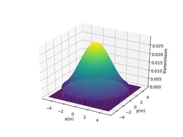
ABSTRACT

The next technological breakthrough in millimeter-submillimeter astronomy is 3D imaging spectrometry with
wide instantaneous spectral bandwidths and wide fields of view. The total optimization of the focal-plane in-
strument, the telescope, the observing strategy, and the signal-processing software must enable efficient removal
of foreground emission from the Earth’s atmosphere, which is time-dependent and highly nonlinear in frequency.
Here we present TiEMPO : Time-dependent End-to-end Model for Post-process Optimization of the DESHIMA
spectrometer. TiEMPO utilizes a dynamical model of the atmosphere and parametrized models of the astro-
nomical source, the telescope, the instrument, and the detector. The output of TiEMPO is a timestream of
sky brightness temperature and detected power, which can be analyzed by standard signal-processing software.
We first compare TiEMPO simulations with an on-sky measurement by the wideband DESHIMA spectrometer,
and find good agreement in the noise power spectral density and sensitivity. We then use TiEMPO to simulate
the detection of the line emission spectrum of a high-redshift galaxy using the DESHIMA 2.0 spectrometer in
development. The TiEMPO model is open source. Its modular and parametrized design enables users to adapt
it to design and optimize the end-to-end performance of spectroscopic and photometric instruments on existing
and future telescopes.

Keywords: Millimeter-wave, Submillimeter-wave, DESHIMA, Spectrometer, Simulation, Kinetic Inductance
Detectors, Astronomical Instrumentation

                                          1. INTRODUCTION

The rapidly growing instantaneous bandwidth1–5 and field-of-view6–8 of millimeter-submillimeter (mm-submm)
astronomical instruments and telescopes are advantageous not only for collecting more astronomical signal, but
also for characterizing and removing the foreground emission of the Earth’s atmosphere.9 Even at the best
sites for submm astronomy on ground, the brightness temperature of the Earth’s atmosphere in the submm
range is ≥20 K, which can be ∼103 –105 times stronger than the astronomical signal (see Fig. 1). Conventional
heterodyne instruments on single-dish telescopes have a typical instantaneous bandwidth of several GHz, which
is sufficiently small compared to the atmospheric “windows” (the frequency bands over which the atmosphere is
relatively transparent). In this narrow-band case, the effect of the atmosphere can often be approximated with
a baseline that is linear in frequency. However, the (ultra-)wideband spectrometers in development, such as the
Deep Spectroscopic High-redshift Mapper (DESHIMA),1, 2, 10 are strongly influenced by the nonlinear frequency
dependence of the atmosphere, because they measure across one or even multiple atmospheric windows with
strong absorption bands in between. On the one hand, this poses new challenges on the observation and signal-
processing techniques to remove the nonlinear atmospheric emission.9 On the other hand, the wideband spectral
information of the atmosphere could enable the development and use of advanced signal processing methods
for characterizing and ultimately removing the atmospheric component to extract the astronomical signal in a
better way. The requirements for applying such techniques are expected to drive the design of future telescopes
and focal-plane instrument systems.6–8
Here we present TiEMPO, the Time-dependent End-to-end Model for Post-process Optimization of the
DESHIMA spectrometer. TiEMPO is a numerical model for simulating wideband submm astronomical observa-
tions through the Earth’s atmosphere, and produces timestream data that can be fed to data-analysis software11
as if they were taken with a real instrument operated on a telescope. To account for the nonlinear, dynamic, and
inhomogeneous transmittance of the atmosphere, TiEMPO utilizes the Atmospheric Transmission at Microwave
(ATM) model12 to simulate the spectral dependence, and the Astronomical Radio Interferometer Simulator
(ARIS) model13–15 to simulate the spatial/temporal variations. TiEMPO is distributed as an open-source Python
package and the scripts are available on a public repository,16 to encourage further use and development by the
astronomical community to study cases for different telescope/instrument systems.
2. THE TIEMPO MODEL
2.1 Overview
TiEMPO is an end-to-end model, containing models of the astronomical source, the atmosphere, the telescope, the
cryogenic instrument optics, and an integrated superconducting spectrometer with microwave kinetic inductance
detectors (MKIDs) (see Fig. 2). The details of the TiEMPO model can be found in Refs.17, 18 and the source code
is publicly available.16 In the following we provide an overview of the modules, in the order of signal propagation
from the astronomical source to the detector.
2.2 Dusty High-redshift galaxy
The galaxy spectrum was created using the GalSpec package,19 which we distribute as an open-source Python
package that can be used outside of TiEMPO. Our goal is to create a galaxy template that is similar to the types
of galaxies we will be trying to detect with DESHIMA, and with which we are able to model the potential future
science cases. As such, we have taken an empirical approach to the creation of a galaxy spectrum, combining the
continuum shape and spectral line luminosities from recent studies of observed local and high-redshift galaxies.
The continuum is based on the two-component modified-black body fit to 24 galaxies at z > 2 with Herschel
(250, 350 and 500 µm ) and SCUBA-2 (850 µm) fluxes.20, 21 Here, we normalize the spectrum to the total
far-infrared luminosity by integrating the spectrum from 8 to 1000 µm. The spectral lines are simulated with
a more creative approach that can be tailored to specific science goals. Relatively shallow observations, aimed1.00
0.75
DESHIMA 2.0
DESHIMA 1.0
ηatm
0.50
0.25
0.00
100
Tsky (K)
PWV=0.5mm
PWV=1.0mm
PWV=2.0mm
10
Flux Density (mJy)
100
TA (mK)
0
10
z = 3.5
¤
z = 4.43
z = 7.5
10
200 300 400 500 600 700 800 900 1000
Frequency (GHz)
Figure 1: Atmospheric transmittance ηatm (top) and sky brightness temperature Tsky (middle) at zenith (θ = 90◦ )
as functions of frequency, for three values of precipitable water vapor (PWV). The instantaneous frequency
coverage of DESHIMA 1.01 and the future DESHIMA 2.0 (see Section 4) are indicated by the green and blue
shades, respectively. The range of DESHIMA 1.0 is an example of one atmospheric “window”. DESHIMA 2.0
spans multiple atmospheric windows with absorption-bands in between. (Bottom) GalSpec-simulated spectrum
of a galaxy with a far-infrared luminosity of LFIR = 1013.7 L , placed at three different redshifts. The spectrum
for z = 4.43 is given as input to TiEMPO in Section 4. The right vertical axis is a rough indication of the
corresponding atmosphere-corrected antenna temperature TA∗ , assuming a ∅10 m telescope with an aperture
efficiency of 0.6.GalSpec
galaxy spectrum
ARIS TiEMPO
Use ARIS deshima-sensitivity
EPL screen ATM
EPL to PWV Atmosphere
look up table
(PWV, f) → eta
beam-
PWV screen averaged T_sky
PWV
Optical Chain:
Telescope
Beam Sampling Warm Optics
Cold Optics
Spectrometer
P_MKID
Detector:
+ photon noise P_MKID + noise
+ quasiparticle noise
P_MKID + noise
Skydip Calibration
DeCode
T_sky + noise
Figure 2: System diagram of TiEMPO, showing each component with its input and output. TiEMPO depends on
external packages ARIS,13, 14 ATM,12 and GalSpec.19 TiEMPO outputs calibrated sky brightness temperature Tsky
and detector output PMKID , which contains photon noise, quasiparticle recombination noise, and atmospheric
noise. The output timestream data can be analyzed by post-processing software such as De:code.11
at detecting atomic lines and CO, are simulated using spectral line luminosity scaling relations. Here we use
the scaling relations from Ref.22 for atomic lines and Ref.23 for both CO and [CI] lines. The scaling relations
of Ref.22 are based on local star-forming and ultra-luminous infrared galaxies and high-redshift submillimeter
galaxies, whereas the scaling relations of Ref.23 are based mostly on local galaxies. Deeper observations might
resolve more complex molecular lines in both emission and absorption, such as H2 O, HCN, HCO+ , CH+ , NH,
NH2 , OH+ , and HF. These species are only incidentally seen at high redshift (e.g., Ref.,24 Berta et al. in prep),
and thus we rely on the line detections in the nearby ULIRG Arp 220 to supplement our spectrum for these
molecular species.25 Here, instead of scaling to the far-infrared luminosity, we scale the line brightness to the
observed continuum at the line’s frequency. For this complete galaxy spectrum, we note that the brightness
of these spectral lines is a probe of the conditions of the interstellar medium. As such, the line brightnesses
(and even the continuum) are known to vary by up to 1 dex from source to source, which must be taken into
account when applying for the necessary observation time or detection limits. Throughout this work, we assumea uniform line velocity width of 600 km s−1 (full width half maximum), which is found to be the mean for typical
SMGs26 and in line with recent observations of South Pole Telescope and bright Herschel sources.27–29
2.3 Creation of the Atmosphere Screen
Our goal here is to obtain the line-of-sight transmittance of the atmosphere ηatm , which depends on the time t
and telescope pointing angle (θ, φ). Here, θ and φ are the elevation and azimuth angles of the telescope pointing,
respectively. We start from the observation that the mm-submm ηatm at zenith (θ = 90◦ ) is correlated with
chiefly one variable, the precipitable water vapor (PWV).30 Water vapor not only absorbs the submm waves,
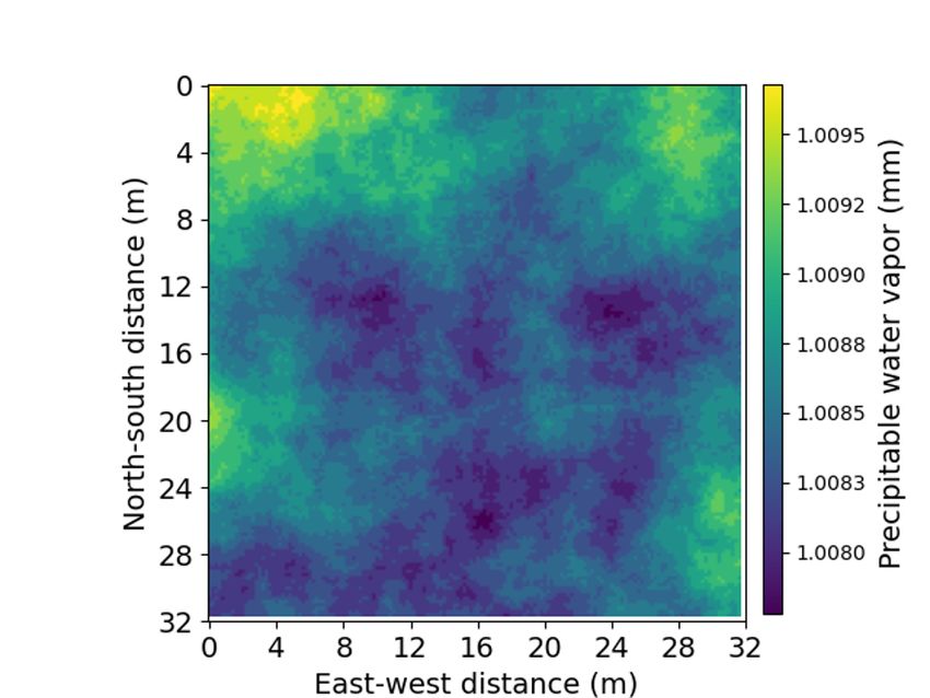
but also introduces an extra path length (EPL) that is dependent on the line-of-sight PWV.31 ARIS13, 14 uses a
set of spatial structure functions32 to produce a phase screen, i.e., a two-dimensional map of EPL as shown in
the left panel of Fig. 3.
TiEMPO converts an EPL screen to a PWV screen, using the following relation derived from the Smith-
Weintraub constants33 of EPL and the ideal gas law (see Ref.17 for details):
k3
dEP L = 10−6 ρR(k2 + ) dP W V ∼ 6.587 · dP W V. (1)
T
Here, k2 = 70.4 ± 2.2 K mbar−1 and k3 = (3.739 ± 0.012) · 105 K2 mbar−1 are the Smith-Weintraub constants,33
ρ = 55.4 · 103 mol m−3 is the number density of molecules in liquid water, R = 8.314 · 10−2 mbar m3 K−1 mol−1
is the gas constant, and T ∼ 275 K is the physical temperature of the atmosphere. Note that dEP L and dP W V
are differences from arbitrary mean values of the optical path length and PWV, respectively. In TiEMPO the
user can specify a mean PWV, around which the PWV fluctuates according to the ARIS-modeled EPL and
Eq. 1. The mean PWV can be set to a constant, or a vector that represents a slowly changing weather condition.
The created PWV screen moves spatially in one direction, at the user-specified wind velocity, assuming that the
structure of phase fluctuations is invariant when the atmosphere moves with the wind.34 See the left panel of
Fig. 3 and the online animation for an example of the moving atmosphere created in TiEMPO.
2.4 Sampling of the Atmosphere by the Telescope Near-Field Beam
The water vapor in the atmosphere above the Atacama Desert is contained mostly in the layer up to ∼1 km from
ground,35 which is well within the near field of the telescope. Therefore, the beam pattern at this height has a
similar pattern to the power distribution over the primary mirror of the telescope. For simulating DESHIMA on
ASTE using TiEMPO, we have assumed a Gaussian power pattern as shown in the right panel of Fig. 3, which
drops to −10 dB at the telescope radius of 5 m. The PWV map created in Subsection 2.3 is filtered with this
beam pattern, so that the received power from the atmosphere is a weighted average within the beam. The user(a) (b)
Figure 3: (Left) Colormap of the output of ARIS for a 32 m × 32 m sky window converted to PWV with Eq. 1.
(v online video) (Right) The truncated Gaussian that is used as the telescope beam shape in the model. The
volume of the Gaussian is normalized to unity, and it is truncated at a radius of 5 m, where its height is 10% of
its peak height.
may include an arbitrary beam pattern in TiEMPO, when detailed information is available from the design or
measurement.
2.5 The Far-Field Beam of the Telescope
The far-field telescope beam is modeled by two properties:36 the main beam solid angle ΩMB and the main beam
efficiency ηMB . ΩMB represents the solid angle of the beam excluding the side lobes. ηMB is the fraction of the
beam contained in the main beam, out of the total reception pattern. The (total) beam solid angle, with the
side lobes included, is then given by
ΩMB
ΩA = . (2)
ηMB
We use the beam solid angle to define the effective aperture area:
λ2
Ae = , (3)
ΩA
where λ is the wavelength. Now, we can express the aperture efficiency ηA as
Ae ηMB λ2
ηA = = , (4)
Ap ΩMB Ap
where Ap is the physical area of the telescope primary mirror. From these quantities, the single-mode power
density (in W Hz−1 ) of the astronomical source is calculated as
1
Pf = Ff Ae , (5)
2where Ff denotes the flux density in W m−2 Hz−1 (= 1026 Jy) and the factor 1/2 compensates for the fact
that the flux density is calculated using two polarizations, but the power density that TiEMPO calculates is
for single-polarization assuming the coupling of the signal to a single-mode (on-chip) antenna and transmission
line.2
2.6 Radiative Transfer
For calculating the single-mode radiation transfer from the astronomical source to the detector, a subset of the
deshima-sensitivity software37 was used. Each component in the optical chain is modeled with a black body
power density and a transmission factor ηi . The single-mode power density of a black body is equivalent to the
Johnson-Nyquist noise, and is given by
hf
Pf = hf . (6)
e kB T
−1
Here, h is the Planck constant, f is the frequency, kB is the Boltzmann constant and T is the physical temperature
of the emitter.38 The spectral power before the detector is computed by cascading the radiation transfer of each
component as:
Pf,out = ηi Pf,in + (1 − ηi )Pf,medium , (7)
where Pf,out is the power density of the radiation that comes out of the component, Pf,in is the power density of
the radiation going in, ηi is the transmittance of the medium, and Pf,medium is the power density of the medium.
2.7 Spectrometer
TiEMPO is able to model any direct-detection (imaging-)spectrometer that couples the wideband input power into
one or more spectral channels. Examples include integrated filterbank spectrometers that use a filterbank1–3
or an integrated grating,4, 5 and optical grating spectrometers. Currently, TiEMPO takes three spatial pixels
to simulate position-switching observations, but the pixel count can be increased to model multi-pixel imaging
arrays. If the number of spectral channels per pixel is set to unity, then the model can represent a monochromatic
imaging camera.
TiEMPO can import the spectral response of each detector, obtained from the design or a measurement.
Here we have assumed a simple Lorentzian-shaped spectral transmission, which is a good approximation for a
filterbank channel,2 or a detector behind an optical (or substrate-integrated) grating.5 The frequency dependence
was implemented by dividing the frequency range of 210–450 GHz (10 GHz wider on each side than the nominal
DESHIMA 2.0 band, to take into account power coupling from outside of the band) into 1500 bins. The resulting
efficiency is used to compute the power density with the radiation transfer equation, Eq. 7. Finally, the powerin each bin is calculated as
Pbin i = ∆f Pf,bin i . (8)
Note that the Pbin i in Eq. 8 is the expected value of the power. To calculate the frequency-integrated power
detected by each detector at each moment t, PMKID (t), we must consider noise (see Subsection 2.8).
2.8 Detected power and noise
The best possible sensitivity of a pair-breaking detector like an MKID is set by the photon noise and quasiparticle
recombination noise. The commonly-used narrow-band approximation for the noise equivalent power (NEP)
limited by photon- and recombination-noise is given by1
q
N EPMKID = 2PMKID (hf + PMKID /∆f ) + 4∆Al PMKID /ηpb . (9)
Here, PMKID is the expected value of the power absorbed by the MKID, ∆Al = 188 µeV is the superconducting gap
energy of aluminium, and ηpb ∼ 0.4 is the pair-breaking efficiency.39 In TiEMPO we use the more general, integral
form of the NEP40 to take into account a frequency-dependent optical efficiency over a wide bandwidth, for each
detector of the spectrometer. Because the fluctuation in energy in different spectral bins are uncorrelated,41 we
can calculate the standard deviation in power for each spectral bin per sampling rate (1/fsampling ) from
r
1
σ = N EPMKID fsampling , (10)
2
and add those together to obtain the combined detector output:
#bins
X
PMKID = Pbin i, with noise (11)
i=1
Note that this is equivalent to calculating the detector NEP directly from the integral:
Z
2
N EPMKID = 2Pf (hf + Pf ) + 4∆Al Pf /ηpb df. (12)
The integration over a wide bandwidth taking the filter spectral transmission into account is especially relevant
for spectral channels that are near strong emission lines and absorption bands of the atmosphere.10
2.9 Sky temperature Calibration
After we have computed the noise-added power that is measured by the MKIDs, we want to relate this back
to the original signal from the sky. We do this by expressing the received power in sky brightness temperature
Tsky : the physical temperature of a black body that would have the same intensity as the semitransparent sky.1
To this end we take the Johnson-Nyquist formula given by
hf
Tsky = . (13)
kB ln( Phff + 1)In order to relate the MKID power PMKID to Tsky , TiEMPO internally performs a skydip simulation10 using
the deshima-sensitivity37 script. A skydip is a series of measurements in which the telescope ‘dips’ from a high
elevation (pointing at zenith) to a low elevation (pointing almost horizontally). When the elevation is lower, the
telescope looks through a thicker layer of atmosphere, increasing the opacity, and hence the power and the sky
temperature, allowing us to construct a relationship between the two. In our simulations, we use elevation values
in the range of θ = 20◦ –90◦ . The power and sky temperature data are interpolated for each channel and saved
in the model. TiEMPO reuses these interpolation curves, so that they only need to be created once. For further
details on the numerical skydip calibration, see Ref.17
3. COMPARING A TIEMPO SIMULATION WITH ON-SKY DESHIMA 1.0
MEASUREMENTS
In order to verify the TiEMPO model, we made a simulation of an atmosphere observation using input parameters
that resemble a real measurement done with the DESHIMA spectrometer on the ASTE telescope.42 DESHIMA
is an integrated superconducting spectrometer with MKID detectors. The first generation of DESHIMA, which
we will hereafter call DESHIMA 1.0,1 has an instantaneous band of 332–377 GHz, with a frequency spacing of
f /∆f ∼ 380. (The half-power bandwidth of each filter is f /∆f ∼ 300 on average.2 ) ASTE is a 10-m Cassegrain
reflector located on the Pampa la Bola plateau of the Atacama Desert in northern Chile, at an altitude of 4860 m.
DESHIMA 1.0 was operated on ASTE during October–November 2017.1 The measured response of the MKIDs
was converted to sky brightness temperature Tsky using a skydip calibration method explained in detail in Ref.10
We use the data taken from a measurement on November 17th 2017, in which the telescope was pointed
close to zenith (θ = 88◦ ) for 3000 s. The PWV measured with the radiometer of the Atacama Large Millimeter-
submillimeter Array (ALMA) was 1.7 mm at the beginning of the measurement, corresponding to a 350 GHz sky
brightness temperature of ∼78 K. In Fig. 4 we show the time-evolution of Tsky taken with the 350 GHz channel
of DESHIMA 1.0 (blue curve). The DESHIMA measurement indicates that the PWV dropped continuously over
the course of the measurement, from ∼1.7 mm to ∼1.3 mm.
The TiEMPO-simulated time trace of Tsky for the 351 GHz channel is compared to that of the DESHIMA 1.0
measurement in Fig. 4. An obvious difference is that the measured curve steadily decreases with time, but the
simulated curve stays at Tsky ∼ 78 K. This is because the TiEMPO-simulation was set to a constant time-averaged
PWV of 1.72 mm. To aid visual comparison of the fluctuations we have included the orange curve in Fig. 4,
which is the observed data but with its linear component subtracted. If we now compare the green (TiEMPO)
and orange (flattened observation) traces, there appears to be a fairly good agreement. Both curves show two82
80
78
76
74
T (K)
72
70
Raw Observation data
68
Observation data without drift
66 Simulation data
0 10 20 30 40 50
Time (min)
Figure 4: Time stream of Tsky , for DESHIMA 1.0 observation (blue) and TiEMPO simulation (green). For better
comparison, the orange trace shows the observation data but with its linear drift subtracted.
Figure 5: Noise power spectral density (PSD) of the simulated and measured sky flux density. The dashed lines
indicate the average level at above 10 Hz where the white photon noise is dominating.
types of fluctuations that are behaving similarly: the low-frequency and large amplitude fluctuations are due to
atmospheric noise, whereas the high-frequency and small amplitude fluctuations are due to photon noise.
To compare the noise in the simulation and measurement more quantitatively, we have taken the power
spectral density (PSD) of the time traces. Before taking the PSD, we have converted Tsky to flux density, by
2ΩMB hf
Ff (Tsky ) = . (14)
ηMB λ2 ηatm e kThfsky − 1Model
VV 114
IRC 10216
beam )
−1
1
10
0.5
NEFD (Jy s
0
10 330 340 350 360 370
Frequency (GHz)
Figure 6: Noise equivalent flux density (NEFD) calculated from the flat photon-noise level (SF ) of the TiEMPO-
simulated data of Fig. 5, compared to the NEFD of DESHIMA 1.0 based on actual detection of astronomical
emission lines, from the luminous infrared galaxy VV 114 and the post-asymptotic giant branch star IRC+10216.1
In Fig. 5 we show the resulting PSDs for the simulation and measurement. At 1 Hz, the PSDs flatten out to the white photon
noise level. This form of PSD is often seen in mm-submm observations.43 The similarity between the two PSDs
indicates that TiEMPO is able to simulate both the atmospheric and photon noise. The photon noise level SF
√
of the observation is 2.6 times higher than that of the simulation, which is consistent with the ×1.6 (∼ 2.6)
difference in the photon noise amplitude in the time stream shown in Fig. 4. This difference suggests a difference
in optical coupling to the sky, which is not surprising because the simulation assumed a constant optical efficiency
and filter half-power bandwidth (f /∆f = 300) for all spectral channels, but the real DESHIMA 1.0 instrument
has channel-to-channel variations in these quantities.2 A more detailed analysis taking into account the measured
characteristics of each channel finds a good agreement in the photon-noise level.44
Using the flat photon-noise level SF calculated from the TiEMPO-simulated PSD, we have calculated the
p
noise equivalent flux density as an indicator of the system sensitivity by N EF D = SF /2. We plot the NEFD
of all 49 simulated channels in Fig. 6, together with the measured NEFD of DESHIMA 1.0 on ASTE based on
actual measurements of astronomical line detection.1 Considering the above-mentioned simplified filter model,
as well as the measurements taken across nights with different atmospheric conditions,1 the agreement is good.
In summary of this section, the output of TiEMPO resembles the on-sky measurement of DESHIMA 1.0, in
both time domain and frequency domain. The end-to-end system sensitivity inferred from the simulation is in
good agreement with the actual measurement of astronomical sources performed by DESHIMA 1.0 on ASTE.4. TIEMPO SIMULATION OF OBSERVING A HIGH-REDSHIFT GALAXY WITH
DESHIMA 2.0 ON ASTE
As an example application of TiEMPO, we simulate the observation of a luminous dusty galaxy (LFIR = 1013.7 L )
at redshift z = 4.43 and velocity width 600 km s−1 using the DESHIMA 2.0 spectrometer on the ASTE telescope.
DESHIMA 2.0 is an upgrade of DESHIMA 1.0, which is currently under development.45 The target instantaneous
frequency coverage is 220–440 GHz, with a frequency spacing and half-power channel bandwidth of f /∆f = 500.
The system will include a rotating mirror in the cabin optics that enables position switching on the sky at a
rate of up to 10 Hz. Assuming the use of this beam chopper, we have simulated a so-called “ABBA” chop-nod
observing technique18, 46 with a beam-chopping frequency of 10 Hz between on-source and off-source positions,
and a nodding cycle of 60 s to subtract the atmospheric emission from the spectrum. The total simulated
observation time was 1 hour. The input spectrum of the galaxy was simulated using GalSpec. The telescope
elevation angle was kept constant at 60◦ , and the weather condition was set to: mean PWV = 1.0 mm; root-
mean-square fluctuation of the EPL σEPL = 50 µm; wind velocity = 9.6 m s−1 .
The resulting spectrum after applying the ABBA atmosphere removal scheme is presented in Fig. 7. The
top panel shows the spectrum in Tsky , that is before correcting for atmospheric absorption. The spectrum shows
the detection of the redshifted [CII] line at 350 GHz, and the dust continuum emission. In the same figure, we
show that a reference simulation without a galaxy yields a zero-centered spectrum as expected. Dividing the
Tsky -spectrum by the frequency-dependent atmospheric transmittance ηatm yields the spectrum presented in the
bottom panel, where the scale is now atmosphere-corrected antenna temperature TA∗ . In this way, TiEMPO
is able to simulate end-to-end observations of future instruments and forecast their scientific products. The
TiEMPO data can also be used to optimize observing strategies and signal-processing techniques before the
instrument is deployed.
5. CONCLUSION AND FUTURE PROSPECTS
We have presented the TiEMPO model and verified its applicability by comparing its output to on-sky measured
data, and simulating the operation of a future instrument. The TiEMPO model is highly parametrized and
modular, so that it can be adjusted to different observation techniques, telescopes, and instruments. This can
be done by either simply adjusting the input parameters, or by relatively simple modifications of the Python
code. For example, some of the authors have adapted TiEMPO to simulate scan-mapping observations,47 or
included excess detector noise.44 TiEMPO can also import arbitrary frequency-dependent transmission curves
from models or measurements, to replace the Lorentzian filter transmission used in this article.44 The time-4 1.0
Galaxy present
No galaxy present
Tsky (mK)
2 True spectrum 0.5
ηatm
0 0.0
4 1.0
TA (mK)
2 0.5
ηatm
*
0 0.0
220 250 275 300 325 350 375 400 425 440
Frequency (GHz)
Figure 7: TiEMPO-simulated detection of a high-redshift dusty galaxy with the upcoming DESHIMA 2.0 instru-
ment on ASTE. The galaxy spectrum was simulated using GalSpec, with input parameters as follows: far-infrared
bolometric luminosity 1013.7 L ; redshift z = 4.43; velocity width 600 km s−1 . The total observing time was
60 min, out of which half was pointing on-source. (Top) The difference in sky temperature Tsky between on-
source and off-source, obtained with the ABBA chop-nod method. The blue spectrum is the result of placing a
galaxy at the on-position, whilst the orange spectrum is the result of no galaxy being present. The dashed curve
is the expected spectrum of the galaxy, multiplied by the atmospheric transmittance ηatm (gray) and smoothed
with a Lorentzian window of f /∆f = 500 to account for the resolving power of the spectrometer. (Bottom)
The atmosphere-corrected antenna temperature TA∗ = Tsky /ηatm . The blue curve shows the simulated spectrum,
whilst the dashed curve is what is expected directly from the input galaxy spectrum.
dependent telescope elevation can be given as a user-specified vector. If the detector is not a pair-breaking type
(e.g., superconducting transition-edge sensors), then the recombination noise term can be omitted in Eq. 9.
It would seem especially interesting to use TiEMPO for the design and optimization of large mm-submm
telescopes, such as the Large Submillimeter Telescope7 and Atacama Large Aperture Submillimeter Telescope
(AtLAST),6 as well as for optimizing instruments and observing techniques on existing large telescopes like the
Large Millimeter Telescope (LMT).48 These telescopes have diameters in the range of 30–50 m, so they sample
a larger column of atmosphere that contains a larger number of patches of water vapor that can influence the
noise behavior. The combination of TiEMPO and ARIS can already simulate observations with telescopes of
these sizes, in combination with the wideband direct detection imaging spectrometers that are considered ascandidates for the future instruments. Note that the current TiEMPO simulates only the transmittance of the
atmosphere, and it does not model the wavefront distortion caused by the dynamical and spatially dependent
EPL. Since ARIS provides an EPL screen, this would be an interesting direction for future development.
6. CODE AVAILABILITY
TiEMPO,16 GalSpec,19 deshima-sensitivity,37 and De:code11 are all available as Python packages and distributed
on a public repository.
ACKNOWLEDGMENTS
We would like to thank Yoshiharu Asaki for providing us with knowledge about the Atacama atmosphere and
the ARIS model, including multiple upgrades of ARIS to enable the use of large phase screens for TiEMPO. We
would also like to thank Henry Kool for the optimization of the computation server used for this study. Most
of the development and validation of TiEMPO was carried out as the TU Delft Bachelor End Projects of EH
and YR. SAB completed the development and published the TiEMPO package as part of her TU Delft Master
End Project. AE was supported by the Netherlands Organization for Scientific Research NWO (Vidi grant n◦
639.042.423). JJAB was the supported by the European Research Counsel ERC (ERC-CoG-2014 - Proposal n◦
648135 MOSAIC). YT was supported by the Japan Society for the Promotion of Science JSPS (KAKENHI Grant
n◦ JP17H06130). The ASTE telescope is operated by National Astronomical Observatory of Japan (NAOJ).
REFERENCES
[1] Endo, A., Karatsu, K., Tamura, Y., Oshima, T., Taniguchi, A., Takekoshi, T., Asayama, S., Bakx, T.
J. L. C., Bosma, S., Bueno, J., Chin, K. W., Fujii, Y., Fujita, K., Huiting, R., Ikarashi, S., Ishida, T.,
Ishii, S., Kawabe, R., Klapwijk, T. M., Kohno, K., Kouchi, A., Llombart, N., Maekawa, J., Murugesan,
V., Nakatsubo, S., Naruse, M., Ohtawara, K., Pascual Laguna, A., Suzuki, J., Suzuki, K., Thoen, D. J.,
Tsukagoshi, T., Ueda, T., de Visser, P. J., van der Werf, P. P., Yates, S. J. C., Yoshimura, Y., Yurduseven,
O., and Baselmans, J. J. A., “First light demonstration of the integrated superconducting spectrometer,”
Nature Astronomy 3, 989–996 (Aug. 2019).
[2] Endo, A., Karatsu, K., Laguna, A. P., Mirzaei, B., Huiting, R., Thoen, D. J., Murugesan, V., Yates, S.
J. C., Bueno, J., Marrewijk, N. v., Bosma, S., Yurduseven, O., Llombart, N., Suzuki, J., Naruse, M., de
Visser, P. J., van der Werf, P. P., Klapwijk, T. M., and Baselmans, J. J. A., “Wideband on-chip terahertz
spectrometer based on a superconducting filterbank,” Journal of Astronomical Telescopes, Instruments, and
Systems 5, 035004 (Jul 2019).[3] Karkare, K. S., Barry, P. S., Bradford, C. M., Chapman, S., Doyle, S., Glenn, J., Gordon, S., Hailey- Dunsheath, S., Janssen, R. M. J., Kovács, A., LeDuc, H. G., Mauskopf, P., McGeehan, R., Redford, J., Shirokoff, E., Tucker, C., Wheeler, J., and Zmuidzinas, J., “Full-Array Noise Performance of Deployment- Grade SuperSpec mm-Wave On-Chip Spectrometers,” Journal of Low Temperature Physics 199(3-4), 849– 857 (2020). [4] Ade, P. A. R., Anderson, C. J., Barrentine, E. M., Bellis, N. G., Bolatto, A. D., Breysse, P. C., Bulcha, B. T., Cataldo, G., Connors, J. A., Cursey, P. W., Ehsan, N., Grant, H. C., Essinger-Hileman, T. M., Hess, L. A., Kimball, M. O., Kogut, A. J., Lamb, A. D., Lowe, L. N., Mauskopf, P. D., McMahon, J., Mirzaei, M., Moseley, S. H., Mugge-Durum, J. W., Noroozian, O., Pen, U., Pullen, A. R., Rodriguez, S., Shirron, P. J., Somerville, R. S., Stevenson, T. R., Switzer, E. R., Tucker, C., Visbal, E., Volpert, C. G., Wollack, E. J., and Yang, S., “The Experiment for Cryogenic Large-Aperture Intensity Mapping (EXCLAIM),” Journal of Low Temperature Physics 199(3-4), 1027–1037 (2020). [5] Barrentine, E. M., Cataldo, G., Brown, A. D., Ehsan, N., Noroozian, O., Stevenson, T. R., U-Yen, K., Wollack, E. J., and Moseley, S. H., “Design and performance of a high resolution µ-spec: an integrated sub-millimeter spectrometer,” Proceedings of the SPIE 9914, 99143O (2016). [6] Klaassen, P., Mroczkowski, T., Bryan, S., Groppi, C., Basu, K., Cicone, C., Dannerbauer, H., Breuck, C. D., Fischer, W. J., Geach, J., Hatziminaoglou, E., Holland, W., Kawabe, R., Sehgal, N., Stanke, T., and van Kampen, E., “The atacama large aperture submillimeter telescope (atlast),” (2019). [7] Kawabe, R., Kohno, K., Tamura, Y., Takekoshi, T., Oshima, T., and Ishii, S., “New 50-m-class single-dish telescope: Large Submillimeter Telescope (LST),” Proc. SPIE 9906, 990626 (Aug. 2016). [8] Aravena, M., Austermann, J., Basu, K., Battaglia, N., Beringue, B., Bertoldi, F., Bond, J. R., Breysse, P., Bustos, R., Chapman, S., Choi, S., Chung, D., Cothard, N., Dober, B., Duell, C., Duff, S., Dunner, R., Erler, J., Fich, M., Fissel, L., Foreman, S., Gallardo, P., Gao, J., Giovanelli, R., Graf, U., Haynes, M., Herter, T., Hilton, G., Hlozek, R., Hubmayr, J., Johnstone, D., Keating, L., Komatsu, E., Magnelli, B., Mauskopf, P., McMahon, J., Meerburg, P. D., Meyers, J., Murray, N., Niemack, M., Nikola, T., Nolta, M., Parshley, S., Puddu, R., Riechers, D., Rosolowsky, E., Simon, S., Stacey, G., Stevens, J., Stutzki, J., Engelen, A. V., Vavagiakis, E., Viero, M., Vissers, M., Walker, S., and Zou, B., “The ccat-prime submillimeter observatory,” arXiv:1909.02587 (2019). [9] Taniguchi, A., Tamura, Y., Kohno, K., Takahashi, S., Horigome, O., Maekawa, J., Sakai, T., Kuno, N., and Minamidani, T., “A new off-point-less observing method for millimeter and submillimeter spectroscopy with a frequency-modulating local oscillator,” PASJ 72, 2 (Feb. 2020).
[10] Takekoshi, T., Karatsu, K., Suzuki, J., Tamura, Y., Oshima, T., Taniguchi, A., Asayama, S., Bakx, T.
    J. L. C., Baselmans, J. J. A., Bosma, S., Bueno, J., Chin, K. W., Fujii, Y., Fujita, K., Huiting, R., Ikarashi,
    S., Ishida, T., Ishii, S., Kawabe, R., Klapwijk, T. M., Kohno, K., Kouchi, A., Llombart, N., Maekawa,
    J., Murugesan, V., Nakatsubo, S., Naruse, M., Ohtawara, K., Pascual Laguna, A. r., Suzuki, K., Thoen,
    D. J., Tsukagoshi, T., Ueda, T., de Visser, P. J., van der Werf, P. P., Yates, S. J. C., Yoshimura, Y.,
    Yurduseven, O., and Endo, A., “DESHIMA on ASTE: On-Sky Responsivity Calibration of the Integrated
    Superconducting Spectrometer,” Journal of Low Temperature Physics 199, 231–239 (Feb. 2020).

[11] Taniguchi, A. and Ishida, T., “De:code.” https://doi.org/10.5281/zenodo.3971538.

[12] Pardo, J. R., Cernicharo, J., and Serabyn, E., “Atmospheric transmission at microwaves (atm): an improved
    model for millimeter/submillimeter applications,” IEEE Transactions on Antennas and Propagation 49(12),
    1683–1694 (2001).

[13] Asaki, Y., Sudou, H., Kono, Y., Doi, A., Dodson, R., Pradel, N., Murata, Y., Mochizuki, N., Edwards,
    P. G., Sasao, T., et al., “Verification of the effectiveness of vsop-2 phase referencing with a newly developed
    simulation tool, aris,” Publications of the Astronomical Society of Japan 59(2), 397–418 (2007).

[14] Asaki, Y., Saito, M., Kawabe, R., Morita, K.-i., Tamura, Y., and Vila-Vilaro, B., “Simulation series of a
    phase calibration schemewith water vapor radiometers for the atacama compact array,” tech. rep., ALMA
    MEMO No. 535 – http://library.nrao.edu/alma.shtml (2005).

[15] Matsushita, S., Asaki, Y., Fomalont, E. B., Morita, K.-I., Barkats, D., Hills, R. E., Kawabe, R., Maud,
    L. T., Nikolic, B., Tilanus, R. P., et al., “Alma long baseline campaigns: Phase characteristics of atmosphere
    at long baselines in the millimeter and submillimeter wavelengths,” Publications of the Astronomical Society
    of the Pacific 129(973), 035004 (2017).

[16] Huijten, E. and Brackenhoff, S. A., “tiempo deshima.” https://doi.org/10.5281/zenodo.4279086.

[17] Huijten, E., “Tiempo: Time-dependent end-to-end model for post-process optimization of the deshima
    spectrometer,” (2020). Delft University of Technology Bachelor’s Thesis, http://resolver.tudelft.nl/
    uuid:5302e10e-3b56-4d4d-a1fd-6a1d58f57abd.

[18] Roelvink, Y., “Simulation of a high-redshiftline-emitting galaxy detection with deshima using tiempo,”
    (2020).    Delft University of Technology Bachelor’s Thesis, http://resolver.tudelft.nl/uuid:
    c878c9d5-f9af-44fd-83c4-a4bd8a7496b5.

[19] Bakx, T. J. L. C. and Brackenhoff, S. A., “GalSpec.” https://doi.org/10.5281/zenodo.4279062.

[20] Bakx, T. J. L. C., Eales, S. A., Negrello, M., Smith, M. W. L., Valiante, E., Holland, W. S., Baes, M.,
    Bourne, N., Clements, D. L., Dannerbauer, H., De Zotti, G., Dunne, L., Dye, S., Furlanetto, C., Ivison,
    R. J., Maddox, S., Marchetti, L., Michalowski, M. J., Omont, A., Oteo, I., Wardlow, J. L., van der Werf,
P., and Yang, C., “The Herschel Bright Sources (HerBS): sample definition and SCUBA-2 observations,”
MNRAS 473, 1751–1773 (Jan. 2018).
[21] Bakx, T. J. L. C., Eales, S. A., Negrello, M., Smith, M. W. L., Valiante, E., Holland, W. S., Baes, M.,
Bourne, N., Clements, D. L., Dannerbauer, H., De Zotti, G., Dunne, L., Dye, S., Furlanetto, C., Ivison, R. J.,
Maddox, S., Marchetti, L., Michalowski, M. J., Omont, A., Oteo, I., Wardlow, J. L., van der Werf, P., and
Yang, C., “Erratum: The Herschel Bright Sources (HerBS): sample definition and SCUBA-2 observations,”
MNRAS 494, 10–16 (Mar. 2020).
[22] Bonato, M., Negrello, M., Cai, Z. Y., De Zotti, G., Bressan, A., Lapi, A., Gruppioni, C., Spinoglio, L.,
and Danese, L., “Exploring the early dust-obscured phase of galaxy formation with blind mid-/far-infrared
spectroscopic surveys,” MNRAS 438, 2547–2564 (Mar. 2014).
[23] Kamenetzky, J., Rangwala, N., Glenn, J., Maloney, P. R., and Conley, A., “L’CO /LF IR Relations with CO
Rotational Ladders of Galaxies Across the Herschel SPIRE Archive,” ApJ 829, 93 (Oct. 2016).
[24] Spilker, J. S., Aravena, M., Béthermin, M., Chapman, S. C., Chen, C. C., Cunningham, D. J. M., De
Breuck, C., Dong, C., Gonzalez, A. H., Hayward, C. C., Hezaveh, Y. D., Litke, K. C., Ma, J., Malkan,
M., Marrone, D. P., Miller, T. B., Morningstar, W. R., Narayanan, D., Phadke, K. A., Sreevani, J., Stark,
A. A., Vieira, J. D., and Weiß, A., “Fast molecular outflow from a dusty star-forming galaxy in the early
Universe,” Science 361, 1016–1019 (Sept. 2018).
[25] Rangwala, N., Maloney, P. R., Glenn, J., Wilson, C. D., Rykala, A., Isaak, K., Baes, M., Bendo, G. J.,
Boselli, A., Bradford, C. M., Clements, D. L., Cooray, A., Fulton, T., Imhof, P., Kamenetzky, J., Madden,
S. C., Mentuch, E., Sacchi, N., Sauvage, M., Schirm, M. R. P., Smith, M. W. L., Spinoglio, L., and Wolfire,
M., “Observations of Arp 220 Using Herschel-SPIRE: An Unprecedented View of the Molecular Gas in an
Extreme Star Formation Environment,” ApJ 743, 94 (Dec. 2011).
[26] Bothwell, M. S., Smail, I., Chapman, S. C., Genzel, R., Ivison, R. J., Tacconi, L. J., Alaghband -Zadeh,
S., Bertoldi, F., Blain, A. W., Casey, C. M., Cox, P., Greve, T. R., Lutz, D., Neri, R., Omont, A., and
Swinbank, A. M., “A survey of molecular gas in luminous sub-millimetre galaxies,” MNRAS 429, 3047–3067
(Mar. 2013).
[27] Reuter, C., Vieira, J. D., Spilker, J. S., Weiss, A., Aravena, M., Archipley, M., Béthermin, M., Chapman,
S. C., De Breuck, C., Dong, C., Everett, W. B., Fu, J., Greve, T. R., Hayward, C. C., Hill, R., Hezaveh,
Y., Jarugula, S., Litke, K., Malkan, M., Marrone, D. P., Narayanan, D., Phadke, K. A., Stark, A. A., and
Strandet, M. L., “The Complete Redshift Distribution of Dusty Star-forming Galaxies from the SPT-SZ
Survey,” ApJ 902, 78 (Oct. 2020).[28] Bakx, T. J. L. C., Dannerbauer, H., Frayer, D., Eales, S. A., Pérez-Fournon, I., Cai, Z. Y., Clements, D. L.,
De Zotti, G., González-Nuevo, J., Ivison, R. J., Lapi, A., Michalowski, M. J., Negrello, M., Serjeant, S.,
Smith, M. W. L., Temi, P., Urquhart, S., and van der Werf, P., “IRAM 30-m-EMIR redshift search of z =
3-4 lensed dusty starbursts selected from the HerBS sample,” MNRAS 496, 2372–2390 (June 2020).
[29] Neri, R., Cox, P., Omont, A., Beelen, A., Berta, S., Bakx, T., Lehnert, M., Baker, A. J., Buat, V., Cooray,
A., Dannerbauer, H., Dunne, L., Dye, S., Eales, S., Gavazzi, R., Harris, A. I., Herrera, C. N., Hughes,
D., Ivison, R., Jin, S., Krips, M., Lagache, G., Marchetti, L., Messias, H., Negrello, M., Perez-Fournon, I.,
Riechers, D. A., Serjeant, S., Urquhart, S., Vlahakis, C., Weiß, A., van der Werf, P., Yang, C., and Young,
A. J., “NOEMA redshift measurements of bright Herschel galaxies,” A&A 635, A7 (Mar. 2020).
[30] Sewnarain Sukul, Y., “Principal component analysis on atmospheric noise measured with an integrated su-
perconducting spectrometer,” (2019). Delft University of Technology Bachelor’s Thesis, http://resolver.
tudelft.nl/uuid:a75fde14-e7fb-401c-9c47-2f954fc5e70c.
[31] Thompson, A., Moran, J., and Swenson Jr, G., “Interferometry and synthesis in radio astronomy, thompson
ri, eisenstein d., fan x., rieke m., kennicutt rc, 2007,” ApJ 657, 669 (2001).
[32] Dravskikh, A. and Finkelstein, A., “Tropospheric limitations in phase and frequency coordinate measure-
ments in astronomy,” Astrophysics and Space Science 60(2), 251–265 (1979).
[33] Smith, E. K. and Weintraub, S., “The constants in the equation for atmospheric refractive index at radio
frequencies,” Proceedings of the IRE 41(8), 1035–1037 (1953).
[34] Gurvich, A., Koprov, B., Tsvang, L., and Yaglom, A., [Atmospheric Turbulence and Radio Wave Propaga-
tion], Nauka, Moscow (1967).
[35] Giovanelli, R., Darling, J., Henderson, C., Hoffman, W., Barry, D., Cordes, J., Eikenberry, S., Gull, G.,
Keller, L., Smith, J., et al., “The optical/infrared astronomical quality of high atacama sites. ii. infrared
characteristics,” Publications of the Astronomical Society of the Pacific 113(785), 803 (2001).
[36] Wilson, T., Rohlfs, K., and Huettemeister, S., [Tools of Radio Astronomy], Astronomy and Astrophysics
Library, Springer-Verlag, Berlin Heidelberg, 5 ed. (2009).
[37] Taniguchi, A., Endo, A., Matsuda, K., Hagimoto, M., Togami, Y., and Brackenhoff, S., “deshima-sensitivity.”
https://doi.org/10.5281/zenodo.4030558.
[38] Nyquist, H., “Thermal agitation of electric charge in conductors,” Physical review 32(1), 110 (1928).
[39] Guruswamy, T., Goldie, D. J., and Withington, S., “Quasiparticle generation efficiency in superconducting
thin films,” Supercond. Sci. Technol. 27, 055012 (May 2014).
[40] Zmuidzinas, J., “Thermal noise and correlations in photon detection,” Applied Optics 42(25), 4989 (2003).[41] Richards, P. L., “Bolometers for infrared and millimeter waves,” Journal of Applied Physics 76(1), 1–24
(1994).
[42] Ezawa, H., Kawabe, R., Kohno, K., and Yamamoto, S., “The Atacama Submillimeter Telescope Experiment
(ASTE),” Proc. SPIE 5489, 763–772 (Oct. 2004).
[43] Monfardini, A., Benoit, A., Bideaud, A., Swenson, L. J., Cruciani, A., Camus, P., Hoffmann, C., Desert,
F. X., Doyle, S., Ade, P. A. R., Mauskopf, P. D., Tucker, C., Roesch, M., Leclercq, S., Schuster, K. F.,
Endo, A., Baryshev, A. M., Baselmans, J. J. A., Ferrari, L., Yates, S. J. C., Bourrion, O., Macias-Perez,
J., Vescovi, C., Calvo, M., and Giordano, C., “A DUAL-BAND MILLIMETER-WAVE KINETIC INDUC-
TANCE CAMERA FOR THE IRAM 30 m TELESCOPE,” ApJS 194 (June 2011).
[44] Marthi, K., “Modelling kinetic inductance detectors and associated noise sourcesr,” (2020). University of
Groningen Internship Report, http://fse.studenttheses.ub.rug.nl/id/eprint/23044.
[45] Pascual Laguna, A., Karatsu, K., Neto, A., Endo, A., and Baselmans, J. J. A., “Wideband Sub-mm Wave
Superconducting Integrated Filter-bank Spectrometer,” in [2019 44th International Conference on Infrared,
Millimeter, and Terahertz Waves (IRMMW-THz)], 1–2, IEEE, Paris, France (2019).
[46] Archibald, E. N., Jenness, T., Holland, W. S., Coulson, I. M., Jessop, N. E., Stevens, J. A., Robson, E. I.,
Tilanus, R. P. J., Duncan, W. D., and Lightfoot, J. F., “On the atmospheric limitations of ground-based
submillimetre astronomy using array receivers,” MNRAS 336, 1–13 (Oct. 2002).
[47] Zaalberg, S., “Establishing a pointing calibration method for deshima using tiempo,” (2020). Delft Univer-
sity of Technology Bachelor’s Thesis.
[48] Hughes, D. H., Schloerb, F. P., Yun, M. S., Chavez, M., Wilson, G. W., Narayanan, G., Erickson, N., Smith,
D. R., Souccar, K., Gale, D. M., Rebollar, J. L. H., Ferrusca, D., Velazquez, M., Sánchez-Argüelles, D.,
Castillo, E., Aretxaga, I., Pope, A., Doeleman, S., Montaña, A., and Gómez-Ruiz, A., “The Large Millimeter
telescope Alfonso Serrano: scientific operation of the LMT 50-m, first results and next steps (Conference
Presentation),” in [Ground-based and Airborne Telescopes VII], Marshall, H. K. and Spyromilio, J., eds.,
10700, International Society for Optics and Photonics, SPIE (2018).You can also read