United States using a multi-tracer approach
←
→
Page content transcription
If your browser does not render page correctly, please read the page content below
Research article
Atmos. Chem. Phys., 22, 5495–5514, 2022
https://doi.org/10.5194/acp-22-5495-2022
© Author(s) 2022. This work is distributed under
the Creative Commons Attribution 4.0 License.

                  Estimation of secondary PM2.5 in China and the
                   United States using a multi-tracer approach
          Haoran Zhang1 , Nan Li1 , Keqin Tang1 , Hong Liao1 , Chong Shi2,3 , Cheng Huang4 , Hongli Wang4 ,
            Song Guo5 , Min Hu5 , Xinlei Ge1 , Mindong Chen1 , Zhenxin Liu1 , Huan Yu6 , and Jianlin Hu1
      1 Jiangsu   Key Laboratory of Atmospheric Environment Monitoring and Pollution Control, Jiangsu Collaborative
       Innovation Center of Atmospheric Environment and Equipment Technology, School of Environmental Science
              and Engineering, Nanjing University of Information Science & Technology, Nanjing, 210044, China
                    2 National Institute for Environmental Studies, Center for Global Environmental Research,

                                                     Tsukuba, Ibaraki, Japan
            3 Institute of Remote Sensing and Digital Earth, Chinese Academy of Sciences, Beijing, 100094, China
          4 State Environmental Protection Key Laboratory of Formation and Prevention of the Urban Air Pollution

                       Complex, Shanghai Academy of Environmental Sciences, Shanghai, 200233, China
                5 College of Environmental Sciences and Engineering, Peking University, Beijing, 100871, China
         6 Department of Atmospheric Science, School of Environmental Studies, China University of Geosciences,

                                                      Wuhan, 430074, China
                  Correspondence: Nan Li (linan@nuist.edu.cn) and Hong Liao (hongliao@nuist.edu.cn)

                                 Received: 14 August 2021 – Discussion started: 5 October 2021
                         Revised: 28 March 2022 – Accepted: 28 March 2022 – Published: 26 April 2022

      Abstract. PM2.5 , generated via both direct emission and secondary formation, can have varying environmental
      impacts due to different physical and chemical properties of its components. However, traditional methods to
      quantify different PM2.5 components are often based on online or offline observations and numerical models,
      which are generally high economic cost- or labor-intensive. In this study, we develop a new method, named
      Multi-Tracer Estimation Algorithm (MTEA), to identify the primary and secondary components from routine
      observation of PM2.5 . By comparing with long-term and short-term measurements of aerosol chemical com-
      ponents in China and the United States, it is proven that MTEA can successfully capture the magnitude and
      variation of the primary PM2.5 (PPM) and secondary PM2.5 (SPM). Applying MTEA to the China National
      Air Quality Network, we find that (1) SPM accounted for 63.5 % of the PM2.5 in cities in southern China on
      average during 2014–2018, while the proportion dropped to 57.1 % in the north of China, and at the same time
      the secondary proportion in regional background regions was ∼ 19 % higher than that in populous regions; (2)
      the summertime secondary PM2.5 proportion presented a slight but consistent increasing trend (from 58.5 % to
      59.2 %) in most populous cities, mainly because of the recent increase in O3 pollution in China; (3) the secondary
      PM2.5 proportion in Beijing significantly increased by 34 % during the COVID-19 lockdown, which might be
      the main reason for the observed unexpected PM pollution in this special period; and finally, (4) SPM and O3
      showed similar positive correlations in the Beijing-Tianjin-Hebei (BTH) and Yangtze River Delta (YRD) re-
      gions, but the correlations between total PM2.5 and O3 in these two regions, as determined from PPM levels,
      were quite different. In general, MTEA is a promising tool for efficiently estimating PPM and SPM, and has
      huge potential for future PM mitigation.

Published by Copernicus Publications on behalf of the European Geosciences Union.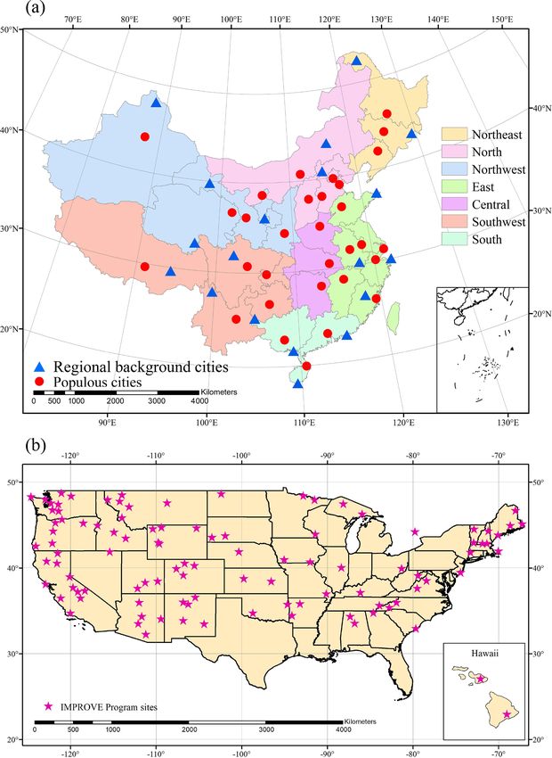
5496                                        H. Zhang et al.: Estimation of secondary PM2.5 in China and the United States

1   Introduction                                                     A chemical transport model (CTM) is another useful tool
                                                                  to identify the composition characteristics of PM2.5 . The sim-
Fine particulate matter (PM2.5 , with an aerodynamic diam-        ulation predicted by a CTM features high spatiotemporal res-
eter of less than 2.5 µm) can be categorized into primary         olution (Geng et al., 2021). Meanwhile, it also provides ver-
and secondary PM2.5 according to its formation processes.         tical profiles of diverse chemical species (Ding et al., 2016).
Primary PM2.5 (PPM), including primary organic aerosol            However, the results of a CTM are largely dependent on ex-
(POA), elemental carbon (EC), sea salt and mineral dust,          ternal inputs such as emission inventories, boundary condi-
is a direct emission product from the combustion of fos-          tions, and initial conditions. The internal parameterizations
sil or biomass fuel, dust blowing and sea spray. Secondary        of itself also significantly influence the final model results
PM2.5 (SPM) is mainly generated by the further oxidation          (Huang et al., 2021), which leads to uncertainty in the sim-
of gaseous precursors emitted in anthropogenic and biogenic       ulated PM2.5 and its composition. In addition, the burden of
activities (Zhu et al., 2018; Wang et al., 2019). SPM con-        their high computational cost and high storage requirement
sists of secondary organic aerosol (SOA) and secondary in-        hinders the universal use of CTMs.
organic aerosol (SIA, including sulfate, nitrate and ammo-           In this study, we develop a novel method, Multi-Tracer Es-
nium). The primary and secondary components of PM2.5              timation Algorithm (MTEA), with the aim of distinguishing
have different environmental impacts on air quality, human        the primary and secondary compositions of PM2.5 from rou-
health and climate change. For example, EC is a typical PPM       tine observation of the PM2.5 concentration. Different from
that can severely reduce atmospheric visibility and greatly in-   traditional CTMs, the MTEA proposed by this study is based
fluence the weather and climate due to its strong absorption      on statistical assumption and works in a more convenient
of solar radiation (Bond et al., 2013; IPCC, 2013; Mao et         way. This algorithm and its application are tested in China
al., 2017). Sulfate, a critical hygroscopic component of sec-     and the United States. In Sect. 2, we introduce the struc-
ondary PM2.5 (SPM), can be rapidly formed in high relative        ture and principle of MTEA. In Sect. 3, we evaluate the
humidity and further leads to grievous air pollution (Cheng et    MTEA results, comparing three PM2.5 composition datasets:
al., 2016; Guo et al., 2014; Quan et al., 2015). Furthermore,     (1) short-term measurements in 16 cities in China from 2012
sulfate and other hygroscopic PM2.5 exert considerable influ-     to 2016, as reported in previous studies; (2) continuous long-
ences on climate change, mostly by changing cloud proper-         term measurements in Beijing and Shanghai from 2014 to
ties (Leng et al., 2013; von Schneidemesser et al., 2015). In     2018; and (3) the IMPROVE network in the United States
addition, different PM2.5 components also have various dele-      during 2014 and 2018. Additionally, we compare the MTEA
terious impacts on human health due to their toxicities (Hu       model with one of the most advanced datasets from a CTM
et al., 2017; Khan et al., 2016; Maji et al., 2018).              in China. Subsequently, in Sect. 4, we investigate the spa-
   To understand the severe PM2.5 pollution characteristics       tiotemporal characteristics of PPM and SPM concentrations
in China over the past several years (An et al., 2019; Song       in China, explain the unexpected haze events in several cities
et al., 2017; Yang et al., 2016), many observational studies      of China during the COVID-19 lockdown, and discuss the
have been conducted on PM2.5 components. The basic meth-          complicated correlation between PM and O3 . This study dif-
ods used in such studies are offline laboratory analysis and      fers from previous works as follows: (1) we develop an effi-
online instrument measurements, such as those made using          cient approach to explore PPM and SPM with low economic
an aerosol mass spectrometer (AMS). Observational studies         or technique costs and a low computational burden, and (2)
are crucial for exactly identifying aerosol chemical composi-     we apply this approach to observation data from the MEE
tions. They represent the most widely used offline approach       (China Ministry of Ecology and Environment) network, of-
(Ming et al., 2017; Tang et al., 2017; Tao et al., 2017; Dai et   fering an unprecedented opportunity to quantify the PM2.5
al., 2018; Gao et al., 2018; W. Liu et al., 2018; Wang et al.,    components at large spatial and time scales.
2018; Zhang et al., 2018; Xu et al., 2019; Yu et al., 2019),
and have been successfully applied to investigate the interan-
                                                                  2     Methodology
nual variations of different aerosol chemical species (Ding et
al., 2019; Z. Liu et al., 2018). In terms of online approaches,   2.1    Multi-Tracer Estimation Algorithm (MTEA)
the AMS is a state-of-the-art method for analyzing different
chemical species with high time resolution, and has great ap-     In order to distinguish PPM and SPM efficiently from the
plication value for diagnosing the causes of haze events in       observed PM2.5 , we develop a new approach, named Multi-
China over the past decade (R. J. Huang et al., 2014; Quan        Tracer Estimation Algorithm (MTEA). The multi-tracer (de-
et al., 2015; Guo et al., 2014; Yang et al., 2021; Gao et al.,    noted X) is defined as representing multiple primary con-
2021; Hu et al., 2021; Zhang et al., 2022).                       tributions to PM2.5 , which mainly results from incomplete
   Nevertheless, both online and offline measurements re-         combustion of carbonaceous material and flying dust. We se-
quire high levels of manpower and are economically costly;        lect the typical combustion product CO as one tracer to repre-
for these reasons, these methods are expensive and rarely ap-     sent the combustion process, and the particles in coarse mode
plied in large-scale regions or for long periods.                 (PMcoarse , denoted PMC, where PMC = PM10 − PM2.5 ) as

Atmos. Chem. Phys., 22, 5495–5514, 2022                                            https://doi.org/10.5194/acp-22-5495-2022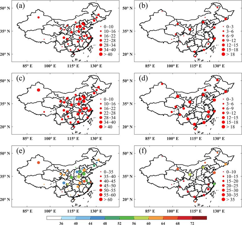
H. Zhang et al.: Estimation of secondary PM2.5 in China and the United States                                               5497

the other tracer to track flying dust. Then we combine the         sions of EC, POA, sulfate and nitrate from the PM2.5 emis-
CO and PMC to generate the multi-tracer X (Eq. 1), which           sions. Based on Eq. (2), we establish a dynamic a and b value
can represent hybrid primary contributions to PM2.5 .              database that reflects the specific changes in PM2.5 sources
                                                                   among years, seasons, hours and regions.
X = a × CO + b × PMC(a + b = 100 %)                         (1)       With the help of the multi-tracer X, we can describe sec-
                                                                   ondary PM2.5 as follows:
As shown in Eq. (1), we use a and b to quantify the rela-
tive contributions of combustion and dust processes to the         SPM = PM2.5 − PPM                                          (3)
PPM. Given that a complicated process such as the com-
                                                                                 PPM
bustion of multiple sources is hard to represent via current           = PM2.5 −     × X.                                     (4)
routine CO observations, we avoid considering the correla-                        X
tion among these sources but focus on the relative weights of      Here, PM2.5 is the observed PM2.5 concentration, and the
the combustion process and flying dust. Meanwhile, the un-         multi-tracer X can be calculated from the observed CO,
certainty resulting from the apportioning coefficients a and       PM2.5 and PM10 concentrations. The original concentrations
b will be further discussed in Sect. 4.5. The values of these      of CO, PM2.5 and PM10 are normalized to avoid any influ-
coefficients depend on the ratio of the emission intensities       ence of their initial levels. To calculate the SPM, the key
of POA + EC (combustion products) and fine-mode dust, as           step is to find the target ratio of PPM/X. In the MTEA
shown below:                                                       method, we give the PPM/X ratio a reasonable range (0–
a   EOA + EEC                                                      400 is used in this work) and then scan the ratio with an
  =                                                                interval of 1. For more precise results, a smaller scanning
b    Efinedust
                                                                   step can be applied, although this may lead to a larger cal-
                   1.2EOC + EEC
  =                                          ,              (2)    culation cost. As a result, each varying ratio may give a se-
      EPM2.5 − (1.2EOC + EEC + ESO4 + ENO3 )                       ries of SPM, along with a coefficient of determination (R 2 )
where EOA , EEC , Efinedust , EOC , EPM2.5 , ESO4 and ENO3         between SPM and X (Fig. S1 in the Supplement). If we as-
represent the emissions of OA, EC, fine-mode dust, OC,             sume that the PPM and SPM came from different sources
PM2.5 , sulfate and nitrate, respectively. We obtain anthro-       or processes, then the appropriate PPM/X ratio should be
pogenic PM2.5 , EC and OC emissions in China from the              the one that corresponds to weak correlation between SPM
Multi-resolution Emission Inventory for China (MEIC, http:         and the tracer X. To aid understanding of the principle of the
//meicmodel.org/, last access: 1 August 2021) developed by         MTEA approach, we show a flow chart in Fig. 1. We also pro-
Tsinghua University (M. Li et al., 2017b). For the United          vide the MTEA software package and input datasets at http:
States, we retrieve the emission data from the global in-          //nuistairquality.com/m_tea (last access: 1 August 2021).
ventory HTAP (https://edgar.jrc.ec.europa.eu/htap_v2/index.           The MTEA approach makes some improvements by using
php?SECURE=123, last access: 1 August 2021). We further            a similar principle and similar assumptions to the modified
estimate the POA emission by multiplying the POC emission          EC-tracer method developed by Hu et al. (2012). They esti-
by an empirical factor of 1.2, as recommended in the litera-       mated primary and secondary organic carbon (denoted POC
ture (Seinfeld and Pandis, 2006), and we quantify sulfate and      and SOC) concentrations by adopting a POC/EC ratio when
nitrate emissions by multiplying the PM2.5 emission by an in-      SOC was least strongly correlated with EC. However, this
vestigative coefficient of 0.1 (Zhang, 2019). However, this in-    assumption may be too hard to achieve in the real atmo-
vestigative coefficient for quantifying primary sulfate and ni-    sphere. Therefore, in the MTEA approach, we take a range of
trate emissions may be relatively high compared to empirical       proper ratios of PPM/X when SPM correlates with the tracer
coefficients (0.01–0.05) used in previous simulation studies.      X nonsignificantly (with a p-value greater than 0.05). As a
We evaluated the potential effect of the coefficient by con-       result, the calculated SPM concentration for each case is a
ducting a set of comparative simulations with a coefficient of     range (Table S2 in the Supplement). We employ the concen-
0.03 and found that the final estimated SPM was not sensi-         tration ranges to represent the severity of secondary pollution
tive to this coefficient (Table S1 in the Supplement). Thus, we    and discuss its uncertainties in the following discussions. For
concluded that the uncertainty of primary sulfate and nitrate      quantitative calculations, the mean values of the concentra-
emissions did not significantly influence the final estimation     tion ranges are used for the final estimation.
of the MTEA model. Other uncertainties of X that are depen-
dent on emission intensities or tracer concentrations are dis-     2.2     PM2.5 measurements
cussed later, in Sect. 4.5. The aim of including coefficient b
                                                                   2.2.1    PM2.5 concentration measurements from the MEE
is to reflect the activity intensity of fine-mode dust by count-
                                                                            network in China
ing the emissions of this dust. However, the MEIC does not
directly provide fine-mode dust emissions. It is included in       Focusing on the PM2.5 pollution in China, MEE set up a
the emissions of total PM2.5 (M. Li et al., 2017a). Thus, we       comprehensive air quality monitoring network that has per-
inferred the fine-mode dust emission by deducting the emis-        mitted consistent access to hourly concentrations of PM2.5

https://doi.org/10.5194/acp-22-5495-2022                                          Atmos. Chem. Phys., 22, 5495–5514, 2022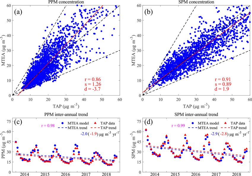
5498                                            H. Zhang et al.: Estimation of secondary PM2.5 in China and the United States

Figure 1. Flow chart of the MTEA approach. The part in red indicates the air quality data and emission input. The part in green represents the
key process for predicting PPM and SPM based on routine PM2.5 observation; in this part, S.T. refers to the significance test. The significant
level α is set to 0.05. The part in orange indicates the final output.

as well as SO2 , NO2 , CO, O3 and PM10 since 2013. This                  formed an evaluation based on two long-term time series of
network is currently the most advanced monitoring network                in situ measurements taken in Beijing (Peking University,
in China. In this study, we obtained hourly surface observa-             PKU) and Shanghai (Shanghai Academy of Environmental
tions of PM2.5 , PM10 , CO and O3 at 334 national monitoring             Sciences, SAES) during 2014–2018 (Huang et al., 2019; Tan
sites in 50 cities from 2014 to 2018 from the MEE public                 et al., 2018). The chemical composition measurements in-
                                                                                                                          2−
website (http://106.37.208.233:20035/, last access: 1 August             cluded ions (NH+         +    +    2+     2+
                                                                                            4 , Na , K Mg , Ca , SO4 , NO3 and
                                                                                                                                 −

2021). Among those 50 cities, 31 are provincial capital cities,          Cl− , measured by ion chromatography), elements (Al, Si, Ti,
which were included to represent populous cities, while the              Ca, Ti, Mn, etc., measured by X-ray fluorescence spectrome-
other 19 are relatively small cities that are categorized as re-         try) and carbonaceous components (EC and organic carbon,
gional background cities (Table S3 in the Supplement). Ex-               measured using a thermal-optical transmittance carbon ana-
cept for Guyuan, the mean PM2.5 concentration in each re-                lyzer). After accessing the chemical compositions, we cat-
gional background city is less than 35.0 µg m−3 (Chinese Na-             egorized them into PPM and SPM for further evaluation.
tional Ambient Air Quality Standard level II, NAAQS), indi-              Specifically, SOA was roughly identified from organic matter
cating that they are only slightly impacted by anthropogenic             (OM) by the EC-tracer model (Ge et al., 2017). SPM concen-
activities. By comparing the populous cities with the regional           trations were calculated by summing the SO2−          −
                                                                                                                        4 , NO3 , NH4
                                                                                                                                     +

background cities, we can reveal the discrepancy in PPM                  and SOA concentrations. Then PPM was calculated by de-
and SPM between regions that suffer from different levels of             ducting SPM from PM2.5 .
PM2.5 pollution. The geographical distribution of these pop-                In addition, we investigated observation-based analyses of
ulous and regional background cities is shown in Fig. 2a.                PM2.5 components in 16 cities in China during 2012–2016
   Recently, the Chinese government carried out a series of              from 32 published studies. This survey offered an opportu-
control policies, such as the elimination of backward in-                nity to compare the estimations from MTEA with past mea-
dustry, desulfurization and denitration of flue gas, as well             surements of the secondary fraction of PM2.5 . SOA concen-
as restrictions on motor vehicles (Tang et al., 2019; Wu et              trations in the literature were roughly estimated by multiply-
al., 2017). Consequently, the concentrations of the major                ing the OM by 0.5 because of limited access to the source
gaseous and particle pollutants have been decreasing year by             data. Meanwhile, it should be noted that the factor that can
year (Zhai et al., 2019; Shen et al., 2020). Taking PM2.5 as             convert OC (organic carbon) to OM is dependent on the def-
an example, previous studies revealed that the annual mean               initions used in a specific observation study.
PM2.5 decreased by 30 %–50 % across China during the pe-
riod of 2013–2018.                                                       2.2.3    PM2.5 composition measurements from the
                                                                                  IMPROVE network in the United States
2.2.2   PM2.5 composition measurements in China
                                                                         The Interagency Monitoring of Protected Visual Environ-
Numerous studies focusing on the aerosol chemical compo-                 ments (IMPROVE) aerosol network has continuous records
sition in China have employed offline filter-based observa-              of PM10 and PM2.5 and PM2.5 chemical speciation in the
tions coupled with laboratory analysis to obtain detailed in-            United States since 1987. The specific aerosol chemical com-
formation on PM2.5 compositions. To directly compare the                 positions include ammonium sulfate, ammonium nitrate, or-
estimated with the measured PPM or SPM in China, we per-                 ganic carbon, EC, soil dust and mineral dust. The catego-

Atmos. Chem. Phys., 22, 5495–5514, 2022                                                     https://doi.org/10.5194/acp-22-5495-2022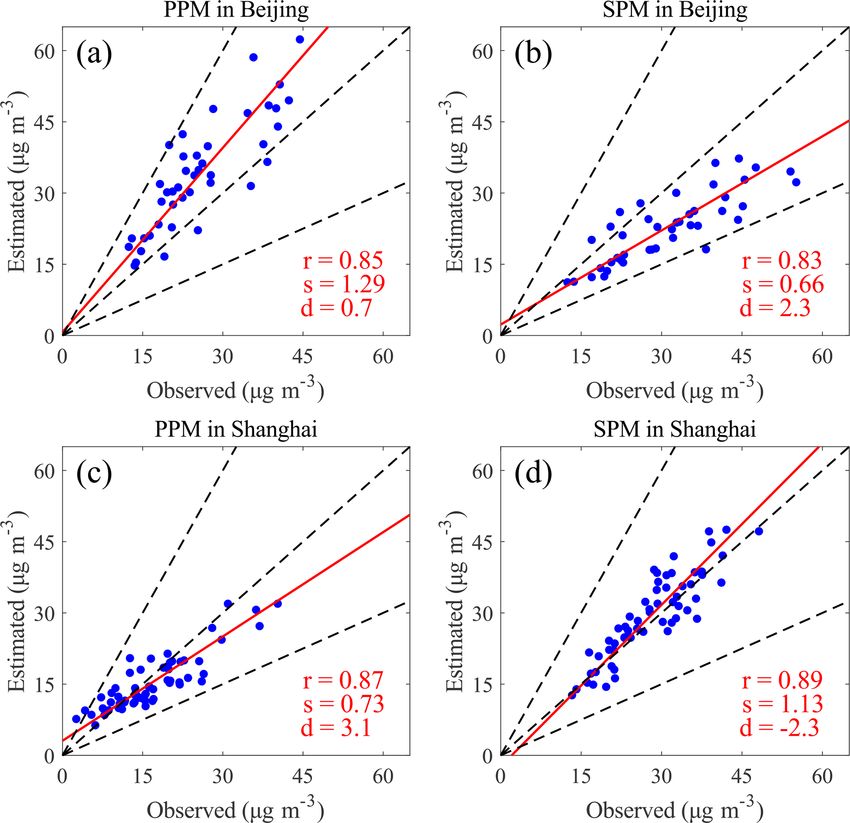
H. Zhang et al.: Estimation of secondary PM2.5 in China and the United States                                                           5499

Figure 2. The geographical locations of the observational data used in this study. (a) Geographical locations of the 31 populous cities (red
circles) and 19 regional background cities (blue triangles) in China considered in this study. (b) Spatial distribution of the IMPROVE aerosol
monitoring network (pink pentagrams) in the United States.

rization process for PPM and SPM in the IMPROVE dataset                  PROVE program only provides a single aerosol component
is similar to the process described in Sect. 2.2.2. The only             profile every 3 d. We lowered the time resolution to the
difference is that the SPM concentration is the sum of am-               monthly average for further evaluation. However, CO is ex-
monium sulfate, ammonium nitrate and SOA. More detailed                  cluded from the IMPROVE program. We therefore adopted
descriptions of IMPROVE are available at http://vista.cira.              the Kriging interpolation of CO data based on the hourly
colostate.edu/Improve/ (last access: 1 August 2021). In the              archives from the United States EPA (https://www.epa.gov/
present study, we extracted measurements for 104 valid sites             outdoor-air-quality-data, last access: 1 August 2021) as an
in the United States from 2014 to 2018 to evaluate MTEA.                 alternative for model input when running MTEA.
The spatial distribution of the IMPROVE sites used in this
work is shown in Fig. 2b. It should be noted that the IM-

https://doi.org/10.5194/acp-22-5495-2022                                                  Atmos. Chem. Phys., 22, 5495–5514, 2022
5500                                          H. Zhang et al.: Estimation of secondary PM2.5 in China and the United States

2.3     PPM and SPM estimated by a CTM
Apart from evaluating PPM and SPM with various compo-
sition measurements, we also compared MTEA estimations
with CTM results. Here, we utilized the PM2.5 composition
gridded dataset with a spatial resolution of 10 km × 10 km
developed by Tsinghua University for further comparisons.
This dataset is named Tracking Air Pollution in China (TAP,
available at http://tapdata.org.cn/, last access: 15 March
2022) (Geng et al., 2021, 2017). The TAP reanalysis dataset
is originally based on CMAQ (Community Multiscale Air
Quality) simulation and is further assimilated by ground
measurements, satellite remote sensing retrievals and emis-
sion inventories with the aid of machine learning algorithm.
We collected the monthly mean concentrations of aerosol
species during 2014–2018 from TAP, including SO2−         −
                                                   4 , NO3 ,
     +
NH4 , OM, BC (black carbon) and total PM2.5 . SOA was
further calculated from OM by the EC-tracer model (Ge et
al., 2017). SPM concentrations were inferred by summing
SO2−       −      +
    4 , NO3 , NH4 and SOA. PPM concentrations were then
obtained by deducting SPM from PM2.5 .
                                                                     Figure 3. Evaluation of the scatter between the monthly mean of
                                                                     the observed PM and that of the estimated PM in Beijing (a–b)
3     Model evaluation                                               and Shanghai (c–d), China. Panels (a) and (c) refer to the PPM,
                                                                     and panels (b) and (d) refer to the SPM. The red numbers in each
3.1     Evaluation in China                                          panel indicate the Pearson correlation coefficient (r), the slope (s)
                                                                     and the intercept of the fit line (d). The red fit lines are based on
3.1.1    Comparison with continuous long-term                        reduced major axis (RMA) regression. The dashed black lines in
         measurements in Beijing and Shanghai                        each panel represent, from left to right, the ratios 2 : 1, 1 : 1 and
                                                                     1 : 2, respectively.
We compared the MTEA results with the two sets of long-
term in situ measurements in Beijing and Shanghai, China,
and the evaluations are shown in Fig. 3. Reduced major axis          a single spot at PKU that is away from crowded streets (Tan
(RMA) regression was applied to fit the data. Given the dis-         et al., 2018). The MTEA predictions based on the data from
crepancy in PM2.5 concentrations between the in situ mea-            MEE sites located in districts with high emission densities
surements at a single site and multiple MEE national sites,          may lead to considerable overestimation of PPM concentra-
we first preprocessed the data for further evaluation. In data       tions.
preprocessing, we removed the in situ daily measurements                Overall, the MTEA model performed satisfactorily in the
with values that were over 30 µg m−3 higher than the city av-        comparison with long-term in situ measurements in Beijing
erage (from MEE).                                                    and Shanghai. Nearly all the points in the plots are located
   Comparisons between the estimated and observed PPM in             at the range between the ratios 2 : 1 and 1 : 2. It is believed
the two cities are given in Fig. 3a and c. The correlation co-       that our model is able to capture the magnitudes and varia-
efficient r for predicted PPM versus observed PPM is 0.85            tions of PPM and SPM. The estimated and the observed in-
for Beijing and 0.87 for Shanghai. The slope of the regres-          terannual variations in PPM and SPM are further compared
sion is 1.29 for Beijing and 0.73 for Shanghai, which indi-          in Sect. 4.2.2.
cates an overestimation (NMB = 32 %) and underestimation
(NMB = −9 %) for these two cities, respectively. For SPM,
                                                                     3.1.2   Comparison with various short-term
the regression line for Shanghai is quite close to the 1 : 1 ratio
                                                                             measurements
line (s = 1.13, d = −2.3), and its statistical correlation is up
to 0.89. The estimated SPM in Beijing also shows a high cor-         To evaluate the reliability of the MTEA approach, we
relation with the observed SPM, with its r value exceeding           also conducted a literature review in which a variety of
0.80, though the fitting formula indicates an underestimation        observation-based analyses of PM2.5 components in 16 cities
of 27 %. These discrepancies can be explained by the fact that       of China during 2012–2016 were collected (Chen et al.,
the observations of primary emission tracers and PM2.5 are           2016; Du et al., 2017; Cui et al., 2015; Dai et al., 2018; Gao
obtained from different sites. Specifically, the CO and PMC          et al., 2018; G. Huang et al., 2014; R. J. Huang et al., 2014;
observations are obtained from 12 monitoring MEE sites in            Huang et al., 2017; Jiang et al., 2017; Li et al., 2016; L. Li
Beijing, while the PM2.5 component measurements are from             et al., 2017; Lin et al., 2016; Liu et al., 2017, 2014; W. Liu

Atmos. Chem. Phys., 22, 5495–5514, 2022                                                 https://doi.org/10.5194/acp-22-5495-2022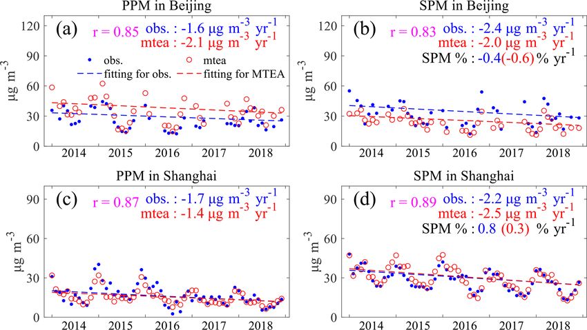
H. Zhang et al.: Estimation of secondary PM2.5 in China and the United States 5501
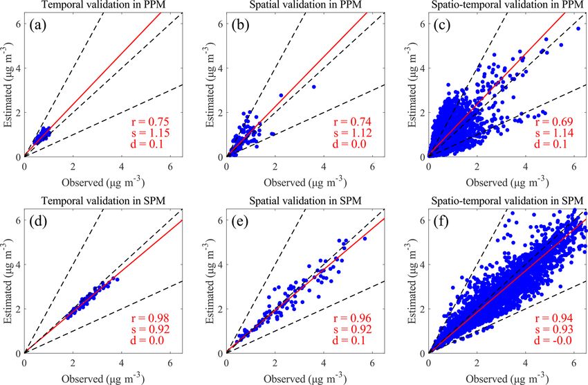
et al., 2018; Z. Liu et al., 2018; Ming et al., 2017; Niu et al., averaged across 31 populous cities (Fig. 4c–d). Both MTEA
2016; Tan et al., 2016; Tang et al., 2017; Tao et al., 2017, and TAP exhibit descending interannual trends in the PPM
2015; Tian et al., 2015; Wang et al., 2018; H. L. Wang et al., concentration, with rates of −2.0 and −1.9 µg m−3 yr−1 for
2016; Y. Wang et al., 2016; Wu et al., 2016; Xu et al., 2019; MTEA and TAP, respectively. For the SPM concentration,
Yu et al., 2019; Zhang et al., 2015, 2018; Zhao et al., 2015). the rates of decline are −2.9 and −2.8 µg m−3 yr−1 , respec-
Most field measurements focused on regions in eastern China tively. Meanwhile, the statistical correlations between the
and on episodes during the winter. We list the observed con- two interannual variations are 0.98 (PPM) and 0.99 (SPM),
centrations of PM2.5 , SO2− − +
4 , NO3 , NH4 and SOA from these which are both quite close to 1, showing good agreement.
studies in Table S4 in the Supplement. It should be noted that Thus, comparisons of the PPM and SPM concentration
there may be inconsistencies between the observations due to magnitudes and interannual variations between the two kinds
differences in sampling locations, observation times and an- of models suggest that our statistical model can infer similar
alytical instruments between studies. estimations to those given by a traditional CTM. Meanwhile,
The estimated PPM and SPM from MTEA show reason- they again highlight that our model is capable of capturing
able agreement with the observation-based PM2.5 component reasonable PPM and SPM concentrations. Furthermore, they
analyses in China. The MTEA-estimated secondary propor- also show that MTEA can track primary and secondary com-
tions of PM2.5 (i.e., secondary PM2.5 / total PM2.5 ) vary in ponents of PM2.5 using a proxy at a much lower cost when
the range of 41 % to 67 % and are higher in eastern cities compared to traditional air quality model simulations.
in China, consistent with the observational results. However,
we find that there are still a few discrepancies between the 3.2 Evaluation in the United States
estimated and observation-based results. For example, we
overestimated the secondary proportions of PM2.5 in cities Based on the chemical component measurements of the
such as Haikou, Lanzhou and Lhasa. Though all of these IMPROVE network, we evaluated the performance of the
show considerable overestimations of over 20 %, the cause MTEA model for the United States. Figure 5 presents scatter
of this bias may be quite different for each city. In the coastal plots of the evaluation results, with the x axis indicating the
city of Haikou, we may attribute this discrepancy between observed concentrations and the y axis indicating the esti-
MTEA and observations to the neglect of the contribution mated concentrations. Temporal, spatial and spatiotemporal
of sea salt aerosols. Offline PM2.5 measurements in 2015 validations were performed. Each dot represents a monthly
showed that the contribution of sea salt aerosols to the ambi- mean observed or estimated PM concentration.
ent PM2.5 mass concentration in Haikou is 3.6 %–8.3 % (Liu Almost all of the dots are located in the region between
et al., 2017). Secondly, the overestimation phenomenon in the 2 : 1 and 1 : 2 dashed lines, indicating that our model is
Lanzhou, which is a typical inland city located in northwest- capable of predicting the magnitudes of PPM and SPM in
ern China, can be explained by the neglect of the contribution the United States. Based on correlation analysis, we find that
of natural dust to PM2.5 speciation. Generally, both sea salt the correlation coefficient r for PPM ranges from 0.69 (spa-
and natural dust are categorized as non-anthropogenic pro- tiotemporal validation) to 0.75 (temporal validation), while
cesses, and are not accounted for by the anthropogenic emis- r reaches up to 0.98 (temporal validation) for SPM. The re-
sion inventory, resulting in an underestimation of the primary sults reveal that the MTEA approach successfully captured
process intensity. Finally, for Lhasa, the observation-based the spatial and temporal variations of PPM and SPM in the
results are derived from too few samplers, leading to a con- United States.
troversial comparison with the MTEA model. The majority of the dots are distributed around the
1 : 1 dashed line. Based on the fitting results, the slopes
3.1.3 Comparison with the CTM simulation
for the regression lines vary from 1.12 (spatial valida-
tion) to 1.15 (temporal validation) for PPM and from
In addition to evaluating our model via PPM and SPM mea- 0.92 (temporal validation) to 0.93 (spatiotemporal vali-
surements in China, we also provide a comparison between dation) for SPM. In general, PPM and SPM show slight
MTEA estimation and CTM simulation for 31 populous overestimation and underestimation, respectively. These
cities based on monthly mean PM concentrations. As shown discrepancies may result from the influences of the emis-
in Fig. 4a–b, the correlation coefficient r for TAP versus sion inventory. It is reported that emissions of PMC and
MTEA is 0.86 in terms of PPM concentration and 0.91 in CO in the United States continuously declined over the
terms of SPM concentration, showing a strongly positive cor- past decade (https://www.statista.com/statistics/501298/
relation between the two models. At the same time, both the volume-of-particulate-matter-2-5-emissions-us/, last ac-
slopes (1.26 and 0.89) and intercepts (−3.7 and 1.9 µg m−3 ) cess: 2 October 2021). Thus, the coefficients a and b derived
of the regressions about PPM and SPM illustrate that most of from the HTAP global emission inventory in 2010 overesti-
the scattered points are distributed around the 1 : 1 ratio line. mate the contribution of primary emissions during the study
Moreover, we further compared MTEA and TAP in terms period. However, these emissions inevitably have an impact,
of the long-term trends in the PPM and SPM concentrations and we will discuss the uncertainty of the emission inventory
https://doi.org/10.5194/acp-22-5495-2022 Atmos. Chem. Phys., 22, 5495–5514, 2022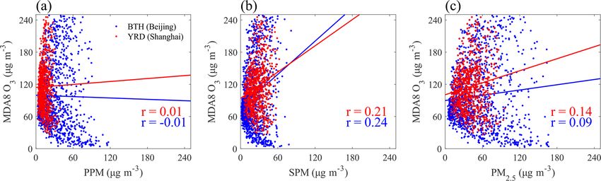
5502                                             H. Zhang et al.: Estimation of secondary PM2.5 in China and the United States

Figure 4. Comparisons between MTEA and TAP in terms of PPM and SPM concentrations and their annual trends from 2014 to 2018 in 31
populous cities in China. In panels (a) and (b), each solid blue dot stands for a monthly mean concentration of PPM or SPM in one of the 31
populous cities. The number of samples is 1860 (60 × 31). The metrics r, s and d represent the correlation coefficient, slope and intercept
of the fit line, respectively. The fitting method used was reduced major axis (RMA) regression. In panels (c) and (d), MTEA and TAP are
denoted by blue circles and red triangles, respectively. Each dot represents the mean PPM and SPM concentration across the 31 populous
cities. The colored numbers show the annual trends in the PPM and SPM concentrations during 2014–2018. The correlation coefficient (r)
of MTEA versus TAP is also provided.

Figure 5. Evaluation of the scatter between the monthly mean of the observed PPM (a–c) or SPM (d–f) and that of the estimated PPM
and SPM in the United States. Panels (a) and (d), (b) and (e), and (c) and (f) show temporal, spatial, and spatiotemporal mixed validations,
respectively. The red numbers in each panel indicate the Pearson correlation coefficient (r), the slope (s) and the intercept of the fit line (d).
The red fit lines are based on RMA regression. The dashed black lines in each panel represent, from left to right, 2 : 1, 1 : 1 and 1 : 2 ratios,
respectively.

Atmos. Chem. Phys., 22, 5495–5514, 2022                                                        https://doi.org/10.5194/acp-22-5495-2022
H. Zhang et al.: Estimation of secondary PM2.5 in China and the United States                                              5503

in Sect. 4.5. In addition, the intercepts of the regression      of their gaseous precursors. Thus, for regional background
lines for both PPM and SPM are less than ±0.1 µg m−3 .           cities, the role of secondary PM2.5 tends to be more impor-
The verification results strongly show that our model can        tant, mainly due to the secondary pollutants transmitted from
reasonably reproduce the monthly averaged concentrations         surrounding populous regions.
of PPM and SPM in the United States.
                                                                 4.2     Temporal variation
4     Results and discussion                                     4.2.1    Seasonal variation
We used the MTEA approach and the MEE observation data           We compare seasonal mean concentrations of the MTEA-
to estimate PPM and SPM concentrations in China for the pe-      estimated PPM and SPM in 31 populous cities and 19 re-
riod of 2014–2018. Observations during severe haze events        gional background cities in Table 1. The concentrations of
(the top 10 % of days for CO and PMC pollution) were ex-         both PPM and SPM are the highest in winter, with a sea-
cluded to avoid the influence of unfavorable meteorologi-        sonal mean concentration of 16.6 for PPM and 24.9 µg m−3
cal conditions and extremely high primary emission cases.        for SPM across China. This phenomenon can be mainly ex-
Unfavorable meteorological conditions are major causes of        plained by adverse diffusion conditions, such as a low bound-
haze events. Under these unfavored meteorological condi-         ary layer height and strong temperature inversion (Zhao et
tions, PPM may have a considerably collinear relationship        al., 2013), as well as fossil-fuel and biofuel usage for win-
with total PM2.5 . The concentration of SPM from compli-         ter home heating (Zhang et al., 2009; Zhang and Cao, 2015).
cated formation pathways is then underestimated. Therefore,      Summer is the least polluted season of the year, with a sea-
we excluded these polluted days to focus more attention on       sonal mean PPM of 10.2 µg m−3 and SPM of 15.8 µg m−3
the general characteristics of the PPM and SPM concentra-        nationwide, largely due to the benefits of a higher boundary
tions.                                                           layer (Guo et al., 2019) and abundant precipitation.
                                                                    We also compared the secondary proportions of PM2.5 in
4.1    Spatial distribution                                      different seasons and in the 50 Chinese cities considered
                                                                 in this work (Table 1). The MTEA approach estimates that
Figure 6 shows spatial patterns of the MTEA-estimated PPM        the secondary proportion tends to be lowest in fall, with a
and SPM concentrations over China averaged for the pe-           seasonal mean value of 56.1 % nationwide, while the sea-
riod of 2014–2018. Sixteen populous cities and nine regional     sonal proportions stay at around 61 % for the other three
background cities in the north, and 15 populous cities and 10    seasons. At the same time, the seasonality of the secondary
regional background cities in the south (the north and south     proportion varies among regions. In the north of China,
are separated by the Qinling–Huaihe line) are involved in the    the secondary proportions are higher in spring and summer,
following discussions.                                           which is attributed to the stronger atmospheric oxidizing ca-
   In populous cities, the concentrations of both PPM and        pacity (AOC) in the warmer seasons. But, in the south of
SPM in the north (the 5-year average is 21.5 for PPM and         China, the highest secondary proportions occur in winter,
26.6 µg m−3 for SPM) are 15 %–43 % higher than those             which is mainly explained by the tremendous amounts of
in the south (the 5-year average is 15.0 for PPM and             pollutants (secondary particles and their gaseous precursors)
23.2 µg m−3 for SPM). The north–south difference is mainly       transported from northern China in the presence of the mon-
caused by the higher energy consumption and consequent           soon.
stronger pollutant emission in northern populous regions.
Nevertheless, in background regions, the difference is rela-
                                                                 4.2.2    Interannual variation
tively small for SPM. The SPM in the south (12.5 µg m−3 ) is
only 1 % higher than that in the north (12.4 µg m−3 ).           Figure 7 illustrates the interannual variations of the estimated
   In terms of the secondary proportion of PM2.5 , the MTEA      PPM and SPM based on MTEA in the 31 populous cities
approach speculates that it is higher in southern regions        and 19 regional background cities of China. We analyzed the
(63.5 %) than in northern regions (57.1 %). This result con-     MEE observational data during 2014–2018 but excluded the
firms the fact that the atmospheric conditions in the south      data for 2014 in the regional background regions due to data
are more favorable for secondary pollutant formation than        deficiencies for several cities.
those in the north. In addition, the MTEA approach cap-            The observed PM2.5 concentrations in populous cities have
tures the difference in the secondary proportion of PM2.5 be-    continuously and significantly reduced since 2014, largely
tween populous and regional background cities reasonably         due to a series of emission control measures led by the
well. As shown in Fig. 6e and f, the secondary proportion        governments, such as the Action Plan on Prevention and
of PM2.5 in regional background cities is 19 % higher than       Control of Air Pollution (Chinese State Council, 2013).
that in populous cities, consistent with recent observational    Using the MTEA approach, we find that both PPM and
studies (Z. Liu et al., 2018). Secondary aerosols can affect a   SPM decreased simultaneously at annual rates of decrease
larger area than primary aerosols, mostly due to the diffusion   of 1.9 and 2.7 µg m−3 yr−1 , respectively. Consequently, the

https://doi.org/10.5194/acp-22-5495-2022                                         Atmos. Chem. Phys., 22, 5495–5514, 2022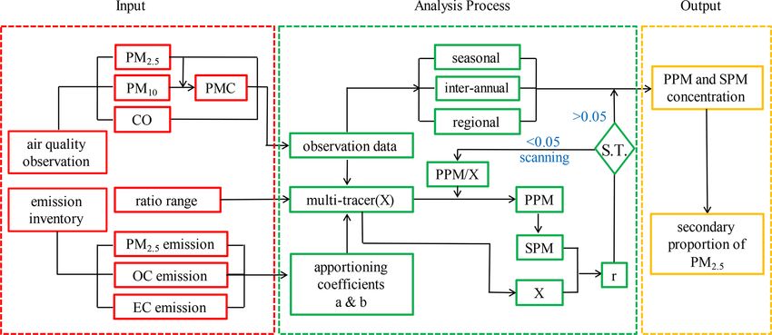
5504                                           H. Zhang et al.: Estimation of secondary PM2.5 in China and the United States

Table 1. Seasonal mean concentrations of primary and secondary PM2.5 in 31 populous cities and 19 regional background cities in China.

                City                   PPM (µg m−3 )                    SPM (µg m−3 )                 SPM/PM2.5 (%)
                                  M       J          S      D     M        J      S       D     M        J      S       D
                                  A       J          O      J     A        J      O       J     A        J      O       J
                                  M       A          N      F     M        A      N       F     M        A      N       F
                Populous cities in northern China
                Beijing         31.0    28.4    30.6      34.1   25.0    23.7   20.1    16.2   44.7    45.4   39.6    32.2
                Tianjin         17.8    13.7    21.9      28.2   42.0    35.3   32.9    29.0   70.2    72.1   60.0    50.7
                Shijiazhuang    35.0    22.4    41.5      54.0   36.7    35.5   32.1    37.7   51.2    61.3   43.6    41.1
                Taiyuan         22.0    20.2    32.7      32.3   28.4    22.2   21.0    25.0   56.3    52.3   39.1    43.6
                Hohhot          13.1    11.4    18.2      20.1   19.2    13.1   16.0    20.7   59.5    53.6   46.8    50.7
                Shenyang        21.0    16.7    24.4      27.8   26.1    17.4   20.8    28.0   55.3    51.0   46.0    50.2
                Changchun       21.3    15.8    20.2      28.9   18.3    12.3   17.2    25.0   46.2    43.9   46.0    46.4
                Harbin          14.1     9.3    15.5      27.2   25.5    15.2   20.9    38.9   64.4    61.9   57.3    58.9
                Jinan           25.6    23.0    29.9      32.4   38.2    30.7   30.7    38.3   59.9    57.1   50.7    54.2
                Zhengzhou       24.8    20.2    28.6      34.1   45.2    28.8   33.9    44.1   64.6    58.7   54.3    56.4
                Lhasa            6.6     5.9     8.2       5.8   13.0     9.2    9.3    13.6   66.3    61.2   53.2    70.1
                Xian            24.1    15.3    31.3      37.1   31.5    20.1   24.5    41.3   56.7    56.7   44.0    52.7
                Lanzhou         14.1    10.1    17.8      21.3   29.3    24.1   24.8    33.2   67.6    70.4   58.2    60.9
                Xining          14.8    12.4    18.3      17.9   26.4    19.3   21.0    34.5   64.1    60.8   53.4    65.9
                Yinchuan        12.9     8.2    16.1      18.7   22.8    21.8   21.1    27.0   63.8    72.8   56.7    59.1
                Urumqi          15.2     9.5    16.5      27.9   30.9    19.1   32.0    63.6   67.1    66.9   66.0    69.5
                Average         19.6    15.2    23.2      28.0   28.7    21.7   23.6    32.3   59.4    58.9   50.4    53.5
                Regional background cities in northern China
                Weihai           8.1     7.1     8.6      10.7   23.8    18.5   14.9    13.7   74.6    72.2   63.4    56.0
                Jiayuguan        7.8     7.0     7.5       7.0   16.6    11.4   14.5    19.2   68.1    61.9   65.9    73.4
                Zhangjiakou     10.8    11.0    10.7      10.7   14.2    14.4   12.8    14.4   56.8    56.6   54.5    57.4
                Daxinganling     4.3     3.6     4.6       5.7    9.2     7.7    9.3    11.6   68.0    67.9   67.0    66.9
                Xilingol         2.3     2.3     2.8       3.1   10.2     9.3    7.7     9.1   81.8    80.1   73.1    74.7
                Yanbian          9.9     5.6     9.4      11.7   15.3     9.1   13.5    17.4   60.7    62.1   58.9    59.7
                Guyuan          12.3     9.0    11.9      13.1   19.0    13.1   14.7    20.1   60.7    59.2   55.4    60.6
                Yushu            4.3     2.1     4.2       3.9   10.0     9.6    7.1     9.9   69.8    82.3   62.7    71.5
                Altay            2.0     1.3     1.7       2.7    6.3     6.3    6.0     8.0   76.1    83.5   77.5    74.7
                Average          6.9     5.5        6.8    7.6   13.8    11.1   11.2    13.7   66.9    67.0   62.1    64.2
                Populous cities in southern China
                Shanghai        12.4    11.1    11.7      15.8   29.5    22.5   20.8    25.4   70.4    67.0   64.1    61.6
                Nanjing         19.1    16.0    19.9      24.3   29.2    18.7   19.9    28.5   60.4    53.9   50.1    54.0
                Hangzhou        21.1    17.8    21.5      23.6   24.9    14.5   18.9    28.5   54.1    45.0   46.8    54.7
                Hefei           16.4    14.6    17.9      23.2   39.8    26.7   30.1    39.8   70.9    64.6   62.7    63.2
                Fuzhou           9.0     7.5     7.5       7.6   18.0    12.9   13.7    19.7   66.6    63.3   64.7    72.2
                Nanchang        14.8     9.8    13.2      15.8   20.6    13.6   22.3    28.8   58.2    58.1   62.9    64.6
                Wuhan           18.5    15.6    18.9      25.3   36.4    19.9   30.0    45.3   66.3    56.1   61.3    64.2
                Changsha        17.6    13.2    17.5      21.9   31.5    21.1   31.2    40.0   64.1    61.5   64.1    64.6
                Guangzhou       11.6     9.5    12.1      12.7   22.6    16.3   23.4    26.6   66.0    63.3   65.9    67.7
                Nanning         11.7     9.7    14.9      13.3   22.0    12.9   19.9    28.7   65.3    57.1   57.1    68.3
                Haikou           5.8     4.7     8.1       6.0   11.5     6.9    8.7    15.8   66.3    59.4   51.8    72.6
                Chongqing       17.9    14.0    18.6      21.6   24.1    19.4   25.0    38.8   57.5    58.0   57.3    64.2
                Chengdu         29.6    20.0    27.1      31.7   23.6    15.0   18.2    39.1   44.3    42.8   40.1    55.2
                Guiyang         13.5    10.6    12.2       9.9   21.3    12.2   18.5    29.8   61.2    53.6   60.4    75.0
                Kunming          9.3     6.5     6.9       8.1   21.1    13.5   16.1    18.4   69.5    67.6   69.9    69.3
                Average         15.2    12.0    15.2      17.4   25.1    16.4   21.1    30.2   62.2    57.7   58.1    63.5

Atmos. Chem. Phys., 22, 5495–5514, 2022                                                    https://doi.org/10.5194/acp-22-5495-2022
H. Zhang et al.: Estimation of secondary PM2.5 in China and the United States 5505
Table 1. Continued.
City PPM (µg m−3 ) SPM (µg m−3 ) SPM/PM2.5 (%)
M J S D M J S D M J S D
A J O J A J O J A J O J
M A N F M A N F M A N F
Regional background cities in southern China
Huangshan 5.3 5.1 5.7 6.4 20.7 11.2 16.3 22.7 79.5 68.8 74.2 78.1
Nanping 6.1 5.0 6.4 5.7 15.9 11.4 13.4 17.4 72.2 69.7 67.9 75.4
Zhoushan 9.5 8.0 8.4 11.9 13.7 10.2 10.1 11.5 59.2 56.2 54.5 49.1
Shanwei 7.9 4.8 8.2 5.7 16.6 10.3 17.4 22.7 67.8 68.2 68.1 79.9
Beihai 7.5 4.2 10.6 8.7 16.4 8.2 16.4 25.8 68.7 65.9 60.6 74.7
Qianxinan 3.3 1.7 2.2 2.9 12.5 12.1 12.2 13.8 79.2 87.9 84.8 82.9
Sanya 4.6 4.2 5.5 3.7 9.7 5.6 6.8 11.7 67.8 56.8 55.4 75.8
Aba 2.0 2.1 2.1 2.9 10.5 10.3 10.3 10.8 84.2 83.0 83.2 78.7
Linzhi 2.3 1.5 2.0 2.1 7.5 6.2 5.3 7.6 76.6 80.5 73.0 78.5
Diqing 1.9 1.5 1.7 1.6 10.5 9.4 9.4 10.2 84.7 86.4 84.8 86.2
Average 5.0 3.8 5.3 5.2 13.4 9.5 11.7 15.4 72.7 71.4 69.1 74.9
Figure 6. Spatial distributions of PPM (a, b), SPM (c, d) and the total PM2.5 concentration (e, f) averaged across the study period. The
secondary proportions of PM2.5 (SPM / total PM2.5 ) are also shown in (e) and (f). The left column (a, c, e) indicates populous cities. The
right column (b, d, f) is for the regional background cities. The dotted black line in each panel shows the Qinling–Huaihe line.
https://doi.org/10.5194/acp-22-5495-2022 Atmos. Chem. Phys., 22, 5495–5514, 20225506 H. Zhang et al.: Estimation of secondary PM2.5 in China and the United States
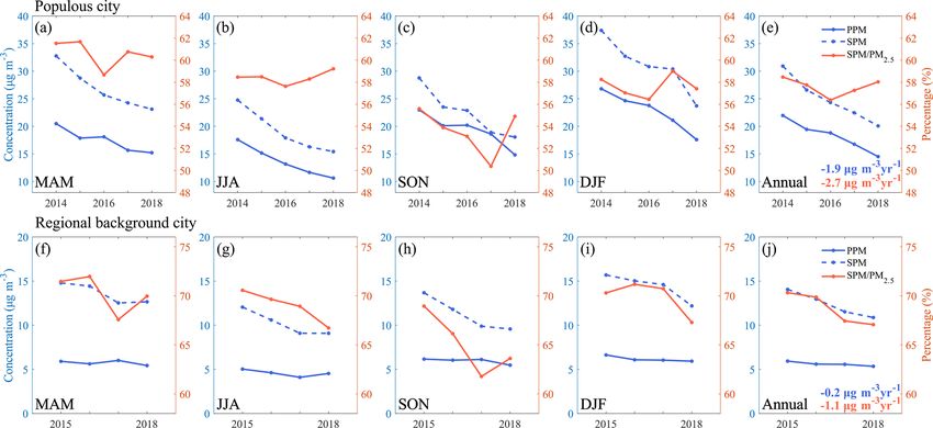
Figure 7. Interannual variations of the PPM concentration (solid blue line), SPM concentration (dotted blue line) and the secondary propor-
tion of PM2.5 (solid red line) in populous cities (a–e) and regional background cities (f–j). MAM (a, f), JJA (b, g), SON (c, h) and DJF (d,
i) denote spring, summer, fall and winter, respectively. The absolute decreases in PPM and SPM concentration are written in blue and red in
panels (e) and (j).
secondary proportion of PM2.5 remains relatively constant it also captures the different trends in the secondary propor-
(56.4 %–58.5 %), but it presents a consistent increasing trend tion of PM2.5 in the two cities (−0.6 % yr−1 in Beijing and
(from 58.5 % to 59.2 %) in summer during the study pe- 0.3 % yr−1 in Shanghai).
riod, which can be attributed to the continuing worsening
O3 pollution (Tang et al., 2022). However, for regional back-
4.3 Application during the COVID-19 lockdown
ground cities, the MTEA approach reports different features
of the PM2.5 mitigation. The estimated SPM is considerably To curb the spread of the novel coronavirus disease 2019
reduced by 1.1 µg m−3 yr−1 in regional background cities, (COVID-19) pandemic, China conducted the first entire city
while the PPM remains nearly unchanged (the rate of de- lockdown in Wuhan, Hubei on 23 January 2020. Other
crease is 0.2 µg m−3 yr−1 ). This is because the SPM in re- provinces also gradually implemented this restriction in
gional background cities is largely contributed by pollutant the following three weeks (Le et al., 2020). The lock-
transport from surrounding populous regions, where the air down greatly limited traffic and outdoor activities, which di-
quality is getting better as a result of the aforementioned rectly reduced the emissions of primary pollutants (Huang
emission controls. However, the PPM mostly derives from et al., 2020). By analyzing the MEE monitoring data ob-
local sources and is rarely affected by those emission con- tained before (1–23 January 2020) and during (24 Jan-
trols, which mostly focus on densely populated and industri- uary to 17 February 2020) the nationwide lockdown (Fig. 9
alized cities, not on background regions. and Fig. S2 in the Supplement), we show that the national
We investigated the interannual variations of PPM and mean NO2 , PM2.5 and CO concentrations were decreased
SPM concentrations on the basis of long-term in situ obser- by 56 %, 30 % and 24 %, respectively, while O3 showed
vations in Beijing and Shanghai as well. As Fig. 8 shows, an increase (of 34 %) in general, which would have effi-
long-term measurements demonstrate a decline in the to- ciently promoted the AOC. However, the surface monitor-
tal PM2.5 by 4.0 µg m−3 yr−1 in Beijing (1.6 for PPM and ing network still observed unexpected PM2.5 pollution in
2.4 µg m−3 yr−1 for SPM) and by 3.9 µg m−3 yr−1 in Shang- cities over the Beijing-Tianjin-Hebei (BTH) region during
hai (1.7 for PM and 2.2 µg m−3 yr−1 for SPM). The observed the lockdown. Especially in Beijing, the mean PM2.5 con-
secondary proportion of PM2.5 shows a slight decrease of centration was increased by ∼ 100 % compared to its average
−0.4 % yr−1 in Beijing but a small increase of 0.8 % yr−1 in value (41 µg m−3 ) before the nationwide lockdown.
Shanghai. Applying the MTEA model to this case, we are Exploring this unexpected air pollution, we find that the
delighted to find that our model not only successfully repro- enhanced secondary pollution could be the major factor;
duces the consistent decreasing trends in PPM and SPM in this even offset the reduction of primary emissions in the
Beijing and Shanghai (the correlation coefficient r of ob- BTH region during the lockdown. With the help of MTEA,
servation versus estimation ranges from 0.83 to 0.89), but we tracked variations of the secondary proportion of PM2.5
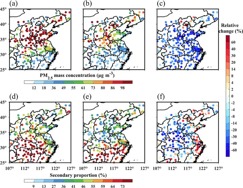
Atmos. Chem. Phys., 22, 5495–5514, 2022 https://doi.org/10.5194/acp-22-5495-2022H. Zhang et al.: Estimation of secondary PM2.5 in China and the United States 5507 Figure 8. The monthly time series variations of PM in Beijing (a–b) and in Shanghai (c–d). Panels (a) and (c) refer to the PPM and panels (b) and (d) refer to the SPM. In each panel, in situ observations and MTEA estimations are shown as blue and red dots, respectively. Meanwhile, the dashed blue and red lines show the long-term trends in concentration changes. The rates of decrease in PPM and SPM concentrations as well as the relative changes in the secondary proportions of PM2.5 (SPM %) are also provided at the upper right corner of each panel. Figure 9. The application of M-TEA to estimate PPM and SPM during the COVID-19 lockdown. Panels (a) and (b) denote the spatial distribution of the PM2.5 mass concentration before the national lockdown (1–23 January 2020, pre-lockdown) and during the national lockdown (23 January to 17 February 2020, post-lockdown). Panel (c) indicates the relative change between panels (a) and (b), i.e., (post- lockdown − pre-lockdown)/pre-lockdown. Panels (d)–(f) are the same as panels (a)–(c) but for the secondary proportions of PM2.5 . https://doi.org/10.5194/acp-22-5495-2022 Atmos. Chem. Phys., 22, 5495–5514, 2022
5508                                         H. Zhang et al.: Estimation of secondary PM2.5 in China and the United States

in East China before and during the COVID-19 lockdown              al., 2020). Because of this significant difference, a question
(Fig. 9d–f). The specific emission reductions owing to the         arises: is the difference mostly caused by PPM, by SPM,
national lockdown were derived from Huang et al. (2020).           or by both of them? To address this question, we com-
Based on bottom-up dynamic estimation, provincial emis-            pared the correlations of daily PPM, SPM and total PM2.5
sions of CO, NOx , SO2 , VOC, PM2.5 , BC and OC decreased          with O3 in the Beijing-Tianjin-Hebei (BTH) and the Yangtze
by 13 %–41 %, 29 %–57 %, 15 %–42 %, 28 %–46 %, 9 %–                River Delta (YRD) regions during the study period with
34 %, 13 %–54 % and 3 %–42 %, respectively, during the             the help of the MTEA approach. The O3 diurnal formation
lockdown period. The secondary proportions in the BTH re-          regime can be destroyed because of the suppressed radia-
gion show evident increases of 7 %–34 %, which highlight           tive condition under precipitation. The local O3 concentra-
the importance of secondary formation during the lockdown.         tion level is mainly dominated by background fields. Here,
Our result is consistent with recent observation and simula-       we would like to focus our attention on the secondary for-
tion studies (Chang et al., 2020; Huang et al., 2020; Le et al.,   mation relationship between daily PM2.5 and O3 . Therefore,
2020) that suggested that the reduced NO2 resulted in O3 en-       the cases during which precipitation took place were re-
hancement, further increasing the AOC and facilitating sec-        moved to avoid the cleaning impacts of wet deposition on
ondary aerosol formation. In addition, another cause of the        MDA8 (maximum daily 8 h average) O3 concentrations. Pre-
air pollution was the unfavorable atmospheric diffusion con-       cipitation data were based on the ERA5 reanalysis database
ditions. CO, a nonreactive pollutant, was increased by 22 %        from the European Centre for Medium-Range Weather Fore-
in Beijing during the lockdown, even given the considerable        casts (ECMWF, https://www.ecmwf.int/, last access: 1 Au-
reduction in its emission.                                         gust 2021).
   For other regions of China, the MTEA approach suggests             As shown in Fig. 10, the correlations between total PM2.5
that the secondary proportion of PM2.5 increased by 20 %           and O3 are positive and stronger in YRD (r = 0.14) than in
over the Yangtze River Delta (YRD) region but decreased by         BTH (r = 0.09). However, compared with total PM2.5 , the
32 % over Central China. Although O3 and AOC enhanced in           correlations between SPM and O3 are much stronger (r =
all these regions, the unprecedented reductions in precursors      0.21–0.24) and show minor regional differences. The corre-
ultimately resulted in a net drop in secondary pollution.          lation of PPM with O3 is not significant (p-value >0.05) in
                                                                   either region. The correlation between SPM and O3 is higher
4.4    Correlation analysis with O3
                                                                   mostly because both of them are secondary oxidation prod-
                                                                   ucts. A higher ambient O3 concentration indicates a stronger
PM2.5 and O3 are closely correlated with each other. One rea-      AOC, which leads to more SPM generation. However, for
son for this is that PM2.5 and O3 have similar precursors, i.e.,   PPM, its effect on O3 is mainly to inhibit the production of
NOx and VOCs. Besides, PM2.5 can impact O3 formation by            O3 by adjusting the radiation balance and affecting the radi-
adjusting the radiation balance (Li et al., 2018) and affect-      cal level. Hence, we suggest that the regional differences in
ing the radical level via aerosol chemistry (Li et al., 2019).     the correlation between total PM2.5 and O3 are mainly caused
There is therefore a complicated interaction between PM2.5         by the different PPM levels in the BTH and YRD regions.
and O3 . Our study utilized the MTEA approach to explore
the relationship between PM and O3 from the perspective of
exploring the statistical correlation.                             4.5   Uncertainties
   Figure S3 in the Supplement illustrates the hourly correla-
tions between the estimated SPM and the observed O3 aver-          Based on the previous evaluation and discussions, we believe
aged for 31 populous cities in China (cities that failed to pass   that MTEA can successfully capture the magnitudes and spa-
the significance test were excluded) in summer. In general,        tiotemporal variations of PPM and SPM in China. However,
SPM and O3 show a positive relationship nationwide, espe-          there are still some uncertainties in the model estimation and
cially during the afternoon (during 14:00–18:00, r is up to        its application in China.
0.56). This phenomenon might be explained by noting that              Firstly, the assumption of nonsignificant correlation be-
the production of O3 and that of SPM are simultaneously            tween PPM and SPM may be violated by the fact that SO2
affected by AOC; thus, a higher correlation tends to occur         and NOx emitted from combustion will further generate
when the AOC is stronger. Moreover, the hourly correlations        secondary sulfate and nitrate particulates. Nevertheless, the
between SPM and O3 are higher than those between PPM               combustion processes for generating SO2 and NOx and PPM
and O3 throughout the day, suggesting that secondary oxida-        are still different. PPM, i.e., BC and POC, mainly comes
tion processes may be captured well by the MTEA method.            from incomplete combustion in residential activities, such as
   A series of recent studies have focused on the correla-         burning biofuels and coal (Long et al., 2013), but SO2 and
tion between PM2.5 and O3 , and many of them have agreed           NOx mainly come from the complete combustion of indus-
that the correlation varies greatly among different regions of     trial and transportation sources, such as coal, gasoline and
China. Specifically, the statistical correlation is more posi-     diesel (Lu et al., 2011; M. Li et al., 2017a; Tang et al., 2019).
tive in southern cities compared to northern cities (Chu et        In addition, the MTEA approach uses the assumption of non-

Atmos. Chem. Phys., 22, 5495–5514, 2022                                              https://doi.org/10.5194/acp-22-5495-2022
H. Zhang et al.: Estimation of secondary PM2.5 in China and the United States 5509 Figure 10. Scatter plots showing the correlation between daily PM concentration and MDA8 O3 concentration in Beijing (blue) and Shanghai (red). Based on the reanalysis dataset ERA5 from ECMWF, days when precipitation took place were removed. Panels (a)–(c) indicate the PPM, SPM and total PM2.5 , respectively. In each panel, solid colored lines represent fit lines based on the least squares method. Values of the Pearson correlation coefficient (r) are also given at the bottom right of each panel. significant correlation rather than irrelevance. Such process- by 10 % and increased the PMC concentration by 10 %. Both ing also reduces the uncertainty to a certain extent. sets of adjustments yield changes of within ±2 % in the es- Secondly, natural sources of PPM, such as fine dust from timated secondary proportions of PM2.5 in all cities except desert and sea salt, are not taken into account in the MTEA for Urumqi (Table S6 in the Supplement). This phenomenon approach. As a result, the PPM in a city near a desert or sea from the perspective of tracer concentration also supports the could be underestimated. For example, the PM2.5 component idea that the impact of the tracer X on the final model results observational campaign conducted in 2015 showed that the is limited. In summary, we believe that the factor that is most contribution of sea salt aerosols to the ambient PM2.5 mass determinative of the final results of our model is the princi- concentration in Haikou is 3.6 %–8.3 % (Liu et al., 2017). ple of minimum correlation between PPM and SPM, not the Thirdly, current bottom-up emission inventories are gener- tracer X, which relies on emissions or concentrations. ally outdated, with a time lag of at least 1–2 years, mainly due to a lack of timely and accurate statistics. Consequently, a corresponding uncertainty in MTEA estimation is inevitable. To evaluate the uncertainty, a comparison test was conducted 5 Conclusions by adjusting the apportioning coefficients (a and b in Eq. 1) with a disturbance of ±0.1. Firstly, we decreased the value of In this study, we developed a new approach, MTEA, to dis- a in each populous city by 0.1. Meanwhile, the coefficient b tinguish the primary and secondary compositions of PM2.5 was increased by 0.1. This scenario indicates an overestima- efficiently from routine observation of the PM2.5 concentra- tion of the contribution of combustion-related processes to tion with a much lower computation cost than traditional the primary PM2.5 or an underestimation of the contribution CTMs. By comparing MTEA results with long-term and of dust-related processes. Secondly, we increased the value short-term measurements of aerosol chemical components of a in each populous city by 0.1 (and decreased b by 0.1) to in China as well as an aerosol composition network in the check the opposite case. The results are presented in Table S5 United States, we showed that MTEA was able to capture in the Supplement, and they point out that the estimated sec- variations of PPM and SPM concentrations. Meanwhile, our ondary proportions of PM2.5 varied by less than ±3 % in the model showed great agreement with the reanalysis dataset most populous cities due to the changes in the apportioning from one of the most advanced CTMs in China as well. coefficients. This sensitivity experiment highlights that the The method was then applied to the surface air pollu- apportioning coefficients, which depend on the emissions, tant concentrations from the MEE observation network in have a limited impact on the final estimation results. Gen- China, and was found to offer an effective way to under- erally, the uncertainty of the apportioning coefficients is one stand the characteristics of PPM and SPM across a wide area. of two factors that directly affect the tracer X. The other one In terms of the spatial pattern, MTEA reveals that SPM ac- is the concentrations of CO and PMC themselves. Hence, we counts for 63.5 % of the total PM2.5 in southern cities aver- also conducted a similar test to check the impacts of tracer aged for 2014–2018, while the proportion drops to 57.1 % X on the model estimation by changing the tracer concen- in the north. It should be noted that the secondary propor- trations mentioned in Eq. (1). Specifically, we (1) increased tion in regional background regions is ∼ 19 % higher than the CO concentration by 10 % and decreased the PMC con- that in populous regions. In terms of seasonality, the esti- centration by 10 % and (2) decreased the CO concentration mated national averaged secondary proportion is the lowest https://doi.org/10.5194/acp-22-5495-2022 Atmos. Chem. Phys., 22, 5495–5514, 2022
You can also read