Wearables Can Afford: Light-weight Indoor Positioning with Visible Light
←
→
Page content transcription
If your browser does not render page correctly, please read the page content below
Wearables Can Afford: Light-weight Indoor Positioning
                       with Visible Light

                                Zhice Yang1†             Zeyu Wang1†
                          zyangab@connect.ust.hk       zwangas@ust.hk
                Jiansong Zhang2          Chenyu Huang3              Qian Zhang1
            jiazhang@microsoft.com      hcyray@gmail.com        qianzh@cse.ust.hk
        1
            CSE, Hong Kong University of Science and Technology 2 Microsoft Research Asia                                            3
                                                                                                                                         Wuhan University
                                                  †
                                                    Co-primary Authors

ABSTRACT                                                                                      Keywords
Visible Light Positioning (VLP) provides a promising means to                                 Indoor Localization; Visible Light Communication; Polarization;
achieve indoor localization with sub-meter accuracy. We observe                               Mobile Devices; Wearables
that the Visible Light Communication (VLC) methods in existing
VLP systems rely on intensity-based modulation, and thus they re-
quire a high pulse rate to prevent flickering. However, the high                              1.   INTRODUCTION
pulse rate adds an unnecessary and heavy burden to receiving de-                                 We envision indoor positioning as being an indispensable feature
vices. To eliminate this burden, we propose the polarization-based                            of smartphones and wearables (e.g., smart glasses) in the near fu-
modulation, which is flicker-free, to enable a low pulse rate VLC.                            ture to support indoor navigation as well as plenty of location based
In this way, we make VLP light-weight enough even for resource-                               services in shopping malls, supermarkets, office buildings, etc. To
constrained wearable devices, e.g. smart glasses. Moreover, the                               realize this goal, we need technologies that can provide high po-
polarization-based VLC can be applied to any illuminating light                               sitioning accuracy as well as being light-weight enough to run in
sources, thereby eliminating the dependency on LED.                                           resource-constrained mobile devices, as these devices (especially
   This paper presents the VLP system PIXEL, which realizes our                               wearables) are normally equipped with CPU, memory and camera
idea. In PIXEL, we develop three techniques, each of which ad-                                that are optimized more for power-efficiency than performance.
dresses a design challenge: 1) a novel color-based modulation scheme                             Visible Light Positioning (VLP) [25, 26] is an emerging posi-
to handle users’ mobility, 2) an adaptive downsampling algorithm                              tioning technique that broadcasts anchor locations through Visible
to tackle the uneven sampling problem of wearables’ low-cost cam-                             Light Communication (VLC). Benefited by densely deployed in-
era and 3) a computational optimization method for the positioning                            door lamps, VLP can easily achieve sub-meter accuracy in indoor
algorithm to enable real-time processing. We implement PIXEL’s                                localization. Compared with Wi-Fi and other RF based approaches
hardware using commodity components and develop a software                                    which normally provide accuracy in meters, VLP holds the promise
program for both smartphone and Google glass. Our experiments                                 for beneficial applications such as retail navigation and shelf-level
based on the prototype show that PIXEL can provide accurate real-                             advertising in supermarkets and shopping malls.
time VLP for wearables and smartphones with camera resolution                                    However, we observe that in existing VLP systems, receiving de-
as coarse as 60 pixel × 80 pixel and CPU frequency as low as                                  vices are heavily burdened in VLC to avoid light flickering, which is
300MHz.                                                                                       caused by their intensity-based modulation method. As human eyes
                                                                                              are sensitive to low rate changes in light intensity, the lamps have
                                                                                              to transmit pulses at a high rate (over 1 kHz) to prevent flickering.
Categories and Subject Descriptors                                                            Since the pulse rate far exceeds the camera’s sampling capability
C.3 [Special-Purpose and Application-Based Systems]: ; C.2.1                                  (30fps), the design of the receiving side has to incorporate hard-
[Computer-Communication Networks]: Network Architecture and                                   ware modification to mobile devices – an additional customized
Design—Wireless communication                                                                 light sensor is required and it relies on cumbersome calibration for
                                                                                              the received signal strength to work properly [26] . A recent inter-
                                                                                              esting idea is to leverage the rolling shutter effect of the CMOS im-
General Terms                                                                                 age sensor to decode high-rate pulses from the high-resolution im-
Algorithms, Design, Experimentation, Measurement                                              age [25, 32, 36]. Although its effectiveness has been shown in high-
                                                                                              end smartphones with high-resolution (40 megapixel) cameras, the
Permission to make digital or hard copies of all or part of this work for personal or
                                                                                              decodable distance is very limited in middle-end smartphones with
classroom use is granted without fee provided that copies are not made or distributed
for profit or commercial advantage and that copies bear this notice and the full cita-
                                                                                              10 megapixel cameras or smart glasses with 5 megapixel cameras.
tion on the first page. Copyrights for components of this work owned by others than           Moreover, the high-resolution image incurs huge computation which
ACM must be honored. Abstracting with credit is permitted. To copy otherwise, or re-          requires a long processing time or cloud off-loading, therefore it
publish, to post on servers or to redistribute to lists, requires prior specific permission   lengthens response time, increases energy cost and sacrifices relia-
and/or a fee. Request permissions from permissions@acm.org.                                   bility.
MobiSys’15, May 18–22, 2015, Florence, Italy.
                                                                                                 The heavy burden on receiving devices motivated us to try to
Copyright is held by the owner/author(s). Publication rights licensed to ACM.
ACM 978-1-4503-3494-5/15/05 ...$15.00.
                                                                                              eradicate the light flickering. Our idea is to modulate the light’s
http://dx.doi.org/10.1145/2742647.2745924.                                                    polarization instead of its intensity for communication. This paper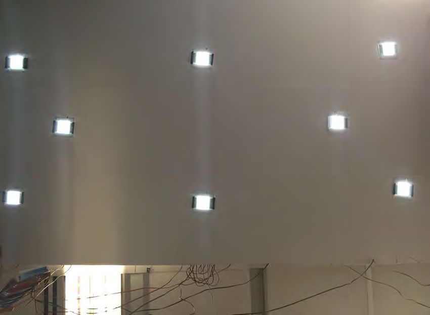
presents our VLP system PIXEL, which realizes this idea. PIXEL           2.    OVERVIEW
enables a light-weight VLP that is even affordable by wearables             This section provides an overview of PIXEL. We first introduce
(Google glass), without incurring hardware modifications or com-         the background of VLP and the flickering problem which motivates
putational off-loading. PIXEL also makes other types of illuminat-       our work. Then we introduce the basics of polarization-based VLC,
ing light beyond LED light (even sun light, §3) usable for transmit-     including techniques for generating/detecting polarized light and
ting location anchors, therefore eliminating the potential barriers to   modulating light’s polarization. Finally, we introduce the idea of
its deployment.                                                          PIXEL’ system which is inspired by the design of one pixel in LCD
   The design of PIXEL’s polarization-based VLC is inspired by the       screen.
Liquid Crystal Display (LCD). We borrow polarizer (§2.2.1) and
liquid crystal (§2.2.2) from LCD as PIXEL’s major components. A          2.1    VLP and the Flickering Problem
challenge in PIXEL’s design is that the SNR in the channel of the           Visible Light Positioning (VLP) relies on Visible Light Commu-
polarization-based VLC differs dramatically in different receiving       nication (VLC) to broadcast location information through modu-
orientations. To address this problem, we propose to add a disper-       lated light beams. The receivers, which are usually mobile devices
sor to PIXEL’s VLC transmitter and employ a novel modulation             carried by humans, use the light sensor [26] or the camera [25] to
scheme, called Binary Color Shift Keying (BCSK) (§3.1). With the         receive the location information as well as measuring their rela-
help of these two modulation techniques, PIXEL is able to achieve        tive position to the lamps to perform fine-grained positioning. The
reliable channel quality despite the user’s mobility. Moreover, on       mechanism is very similar to Wi-Fi positioning except that the vis-
the receiving side, PIXEL also incorporates novel system designs to      ible light is used as the carrier to carry beacon messages instead of
combat the uneven sampling in low-cost cameras (§3.2). The idea          the microwave signal. Benefiting from the high density of the in-
is to exploit the operating system’s clock to obtain more accurate       door lamps, visible light positioning can achieve much better (sub-
timing for video frames. Finally, in order to make the system as         meter level) accuracy than Wi-Fi positioning.
light-weight as possible, we optimize all the algorithms and their          A major headache in VLP is the flickering problem. In current
implementations. Particularly, we optimize the implementation of         VLP designs, communication is based on modulating the light’s in-
the camera-based localization algorithm and achieve orders of mag-       tensity. Optical pulses are generated and data bits are encoded using
nitude performance gain (§3.3).                                          pulse rate or pulse width. The varying light intensity causes flick-
   We prototype PIXEL’s transmitters with commodity components           ering which can make people uncomfortable or even nauseous [19,
and develop a communication and localization program for both            34]. In order to avoid the negative impact of flickering, a high pulse
Android smartphone and Google glass. Our experiments based on            rate has to be used to make the pulses unnoticeable, though the mes-
the prototype system show:                                               sage size required for localization is small. For example, the exist-
                                                                         ing designs use over-1kHz pulse rates to transmit 7-bit beacons [25]
• We enable polarization-based VLC between PIXEL’s transmit-             or over-10kHz pulse rates to transmit 16-byte beacons [26].
  ters and camera-equipped smart devices. Reliable communica-               The forced high pulse rate indeed adds a heavy burden to re-
  tion over a long distance of 10-meters only requires an image/video    ceiving devices. Considering the camera as the most common vis-
  capturing resolution of 120 pixel×160 pixel.                           ible light sensor, the normal frame rate of 30 frames per second
• We enable a fast positioning algorithm in mobile devices. Our          (fps) [22] is much lower than the pulse rate, which means it is far
  optimization reduces the processing time of the camera-based           from sufficient to recover the transmitted pulses if we take one light
  positioning algorithm by three orders, from seconds to millisec-       intensity sample from every frame1 . An interesting idea to tackle
  onds.                                                                  this problem is to leverage the rolling shutter effect of CMOS image
                                                                         sensor [25, 36]. The effect means rather than scanning a scene all
• We enable realtime visible light positioning in resource-constrained
                                                                         at once, the image sensor scans one line at a time. Rolling shutter
  devices and the average positioning time is less than 3 seconds.
                                                                         increases the sampling rate by up to thousands of times (from tens
  Even when the CPU frequency is as low as 300MHz, PIXEL’s
                                                                         of fps to tens of thousands of lines per second), therefore making it
  light-weight design works properly.
                                                                         possible to cover the pulse rate. However, according to our expe-
                                                                         rience, the usefulness of rolling shutter is limited for two reasons.
   In this paper, with the design of the PIXEL system, we make           First, the camera must have very high resolution if it is not close
following contributions:                                                 enough to the lamp. This is because the lamp is only a small por-
                                                                         tion of the image, but a certain number of occupied lines/pixels are
• We identify the problem in existing VLP systems - the heavy            required to carry a message. In other words, if the receiving de-
  burden on receiving devices, and propose a polarization-based          vice does not contain a high-resolution camera, the communication
  VLC to address it. As far as we know, we propose the first system      distance will be short. For example, on a Samsung Galaxy 4 with
  design that leverages polarization-based VLC in open space.            a 13-megapixel camera, we can reach up to 1.6 meters, and with
• We propose to add a dispersor to the VLC transmitter and de-           Google glass’s 5-megapixel camera, we can reach up to 0.9 meters.
  velop a novel VLC modulation scheme called BCSK. These two             Second, processing high-resolution image requires very high com-
  techniques make it possible for the system to provide reliable         putational power. As a consequence, the existing design [25] re-
  communication despite the device’s mobility.                           lies on a cloud/cloudlet server to process the image and decode the
• We develop a novel OS-clock based downsampling scheme to               message. Besides camera and rolling shutter, another solution [26]
  handle the uneven sampling problem of cameras.                         leverages a customized light sensor which is capable of taking high-
                                                                         rate samples on light intensity. Different from camera-based solu-
• We optimize the implementation of the VLC receiving program
  and the positioning algorithm, thereby making the system light-        1
                                                                           Even cameras specially designed for capturing slow-motion video,
  weight enough for smartphones and wearables.                           for example, the 240-fps camera in the latest iphone6, the frame rate
                                                                         is still not sufficient to cover the over-1kHz or higher pulse rate. We
• We implement a prototype of PIXEL and conduct a systematic             also do not expect this slow-motion capable camera to be widely
  evaluation on it. Experimental results validate our design.            equipped into low-end phones and wearables.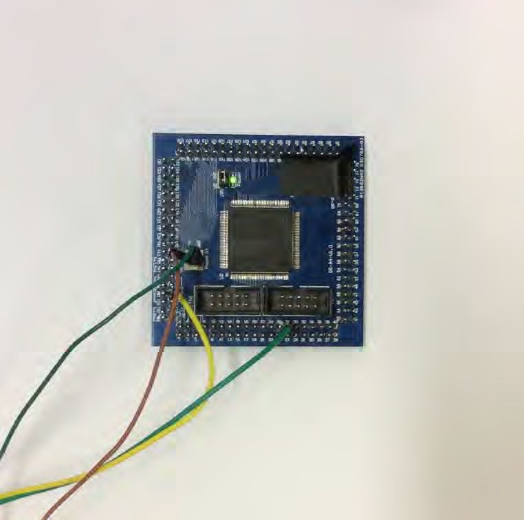
0V

                                                                            Polarized
      Light
                                                                            Light                                                         Dark
      Source
                                                                                                             3V

                                                                                                                                          Bright
       Figure 1: Generating and detecting polarized light.

tions which use the angle-of-arrival based positioning algorithm,               Figure 2: Modulating polarization to encode bits.
the light sensor based solution relies on received signal strength
(RSS) technique to estimate the distance, this however are difficult
to calibrate. Both hardware customization and RSS calibration are       of converting unpolarized light into polarized light by considering
heavy burdens for VLP clients.                                          unpolarized light to be a mix of polarized light with all possible
   Finally, high-pulse-rate VLC also requires the transmitter to be a   polarizations. Figure 1 illustrates the process of generating and de-
Light-Emitting Diode (LED), therefore, lamp replacement is needed       tecting polarized light according to Malus’ law.
if the existing lamps are not LED.
   In this paper, we propose to exploit light polarization to realize   2.2.2     Modulating light’s Polarization
low-pulse-rate VLC, so as to avoid the heavy burdens mentioned             Modulating polarization of visible light using liquid crystal (LC)
above and enable a light-weight VLP design that is affordable on        is also a mature and inexpensive technique. In this paper, we use
wearable devices.                                                       Twisted Nematic (TN) liquid crystal which is very popular in the
                                                                        LCD screens of personal computers, digital watches, etc. TN liquid
2.2     Basics of Polarization Based VLC                                crystal costs only $0.03 per cm2 or $1.5 per lamp in our design.
   Polarization is a property of light waves that they can oscillate       We explain how to modulate polarization to encode bits using
with more than one orientation. Similar to oscillating frequency        Figure 2. The two surfaces, between which a variable voltage is ap-
which is another property of light, polarization preserves during       plied, are the surfaces of a TN liquid crystal layer. TN liquid crystal
light propagation in the air. However, different from oscillating       has the characteristic that when a voltage is applied, its molecules
frequency which determines color and thus can be perceived by hu-       will be realigned – twisted/untwisted at varying degrees depend-
man eyes, light’s polarization is not perceptible [21]. This human-     ing on the voltage. Most commodity TN liquid crystal components
imperceptible nature has been proved very useful in that the po-        are manufactured to have a 90◦ twist when no voltage is applied.
larization has led to the invention of Liquid Crystal Display (LCD)     Therefore a beam of polarized light will be rotated by 90◦ while
techniques, in which screens indeed always emit polarized light [39].   passing through the liquid crystal, as shown in the upper sub-figure.
   In the following subsections, we introduce two basic techniques      If we use a polarizer parallel to the incident light to detect the light,
in polarization-based VLC which solve the problems of generat-          as shown in the figure, the light will be entirely blocked by the po-
ing/detecting polarized light and modulating light’s polarization.      larizer. Then when we increase the voltage, the liquid crystal will
                                                                        untwist and the polarizer will become brighter. Once a certain volt-
2.2.1     Generating/Detecting Polarized Light                          age level is reached, e.g. 3V as in the figure, the liquid crystal will
   Most of the common light sources, including sun light and man-       become totally untwisted and the polarizer will show the brightest
made lighting systems, e.g. fluorescent light, incandescent light,      state. In this way, we can tune the applied voltage to modulate the
etc., produce unpolarized light which contains light of mixed polar-    polarization and encode ‘0’ and ‘1’ using dark and bright states3 .
ization. The technique to convert unpolarized light into polarized
light, called polarizer, is mature and very inexpensive. For exam-      2.3     PIXEL – A Pixel of LCD
ple, the polarizer we use in this paper is a thin film, which costs        Our system, PIXEL, is inspired by the design of the pixels in
roughly $0.01 per lamp. Polarizer is also widely used to detect         LCD. As shown in the upper sub-figure of Figure 3, a pixel of LCD
polarized light and filter out certain unwanted light2 . The theory     consists of two polarizer layers and a liquid crystal layer in between.
behind polarizer is the Malus’ law. That is, if the polarized light     The backlight generates unpolarized light which is converted into
incident to a polarizer has intensity I0 , the passed light will have   polarized light by polarizer 1. The liquid crystal layer twists/un-
intensity Iθ , which is determined by the bearing angle θ between       twists the light’s polarization according to the applied voltage. Po-
the polarization of the light and the polarizing direction of the po-   larizer 2 has a fixed angle of 90◦ in the polarizing direction with po-
larizer:                                                                larizer 1. Therefore, the strength of the emitted light is controlled
                          Iθ = I0 cos2 θ                         (1)    solely by the voltage applied on the liquid crystal layer. Finally,
                                                                        a lot of pixels each of which has an independent control voltage
Therefore, if the incident light has polarization in a direction par-   constitute an LCD screen.
allel to the polarizer, i.e. θ = 0, the light will pass through the        The lower sub-figure illustrates the VLC design of PIXEL. We
polarizer without being attenuated. Otherwise, if their directions      convert a lamp into PIXEL’s VLC transmitter by adding a polar-
are perpendicular, i.e. θ = 90◦ , the incident light will be entirely   izer and a liquid crystal layer. The transmitter thus emits polarized
blocked by the polarizer. Malus’ law can be applied to the case
                                                                        3
                                                                          In theory, we can encode more bits using multiple levels of bright-
2
 For example, both polarized sunglasses and photographic polariz-       ness. However, in this paper we only encode 1 bit to get rid of
ing filter are used to eliminate unwanted reflections.                  complicated calibration.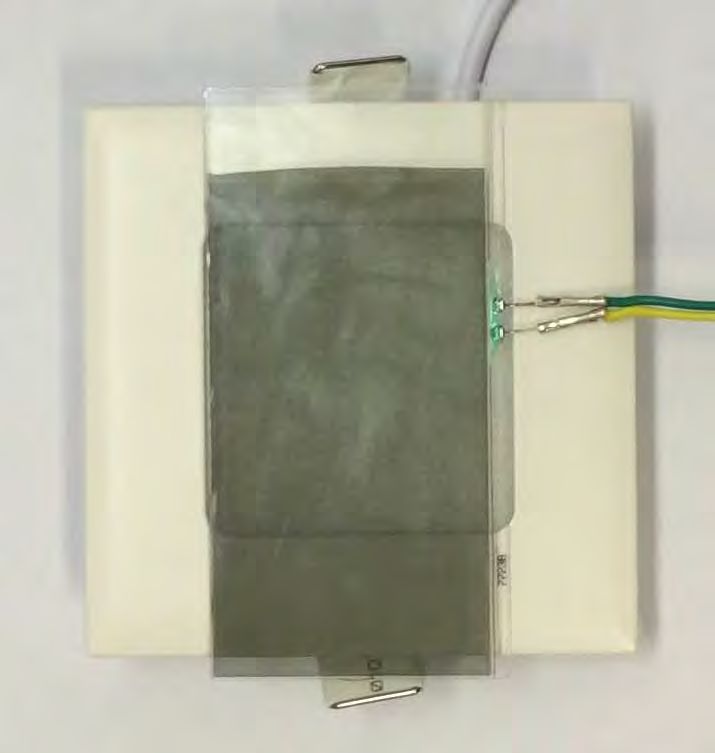
direction                                                                                           VLC
                           difference                                                                                      Transmitter
                              = 90o                                                                                           §3.1
  Liquid
                                                                                         id2     id3
  Crystal                                                                                                id4
  Display         back                                                           id1
                  light
                                                                                                                   Video Preview
             polarizer 1   liquid crystal polarizer 2
                                                                                               or                               VLC
                                    dispersor                                                                    Lamp
                                                                                                                              Receiver
                                                                                                               Locations
                                                                                                                                §3.2
     PIXEL                                                or                                                     AoA Localization &
                 lamp                                                                                             Orientation §3.3

                 VLC transmitter                     VLC receiver
                                                                                           Figure 4: PIXEL Architecture.
       Figure 3: PIXEL is inspired by the design of LCD.

                                                                         ceiving device are determined using angle-of-arrival (AoA) based
light. Light’s polarization can be changed by the voltage applied        algorithms.
to the liquid crystal layer. The change of light’s polarization can-        In PIXEL, it is possible to make use of any type of visible light
not be perceived by human eyes4 or directly captured by cameras.         source to construct a location beacon. As illustrated in Figure 4,
PIXEL’s VLC receiver is a mobile device which equips a camera,           a location beacon may consist of a lamp (not just the LED lamp,
e.g. smart glasses and smartphones. We add another polarizer to          but any lamp) and a PIXEL’s VLC transmitter. A location beacon
the camera for the purpose of detecting the changes of light polar-      may also consist of a window with incident sun light and a PIXEL’s
ization. As discussed in §2.2.2, the polarizer converts polarization     VLC transmitter.
changes into brightness changes that can be captured by the camera.         In the following of this section, we elaborate on three main com-
We notice that the effect of adding polarizer to the camera, consid-     ponents of PIXEL, i.e. VLC transmitter, VLC receiver and the AoA
ering normal photo taking and video recording, is very similar to        based localization/orientation algorithm, to explain the challenges
the use of polarizing filter in photography [28], i.e., the polarizer    as well as our solutions in the design.
does not bring noticeable changes except a slightly reduction in the
strength of the ambient light.                                           3.1     VLC Transmitter
   However, from Figure 3, we can observe an important difference           The VLC design in PIXEL is borrowed from LCD, as has been
between PIXEL and LCD. In PIXEL, the polarizing direction be-            described in §2.3. The VLC transmitter contains a polarizer and
tween polarizer 1 and polarizer 2 does not always remain constant,       a liquid crystal layer that can convert the unpolarized illuminating
because the receiving device may move and rotate with the person         light into polarized light and modulate the light’s polarization using
who holds it. This varying angle is one of the major challenges          a control voltage. Then when the light propagates to receiving de-
in our design. In the worst case the receiving camera will capture       vices, polarization changes will be converted into intensity changes
almost the same light intensity in the two polarization states. To       by another polarizer and identified by the receiving camera. Fi-
tackle this problem, we leverage the camera’s ability of capturing       nally, the VLC transmitter also contains a simple electronic module
chromatic images and add a dispersor to disperse light of different      to encode information, which translates the beacon’s location iden-
colors to different polarizations. The details as well as other chal-    tity into a series of control voltages.
lenges and solutions are elaborated on in the next section.                 A big challenge to PIXEL’s VLC comes from the receiver’s mo-
                                                                         bility, as has been briefly mentioned in §2.3. Unlike the two fixed
                                                                         polarizers in LCD, in PIXEL, though the polarizer in VLC trans-
3.     PIXEL DESIGN                                                      mitter is fixed (attached to the lamp), the polarizer in the receiver is
   PIXEL presents a system design which makes visible-light based        mobile. Therefore, the two polarizers could end up with arbitrary
accurate indoor positioning affordable in wearables and low-end          angles in their polarizing directions. Since this angle determines
smartphones. As shown in Figure 4, every location beacon periodi-        the intensity of light, which is finally captured by the receiving
cally sends out its identity through visible light communication. A      camera, angle ambiguity will lead to a varying intensity difference
wearable device or smartphone captures multiple beacons using the        (intensity-diff) between ‘1’ and ‘0’ states, meaning varying signal-
camera’s video preview. Relative locations of beacons are obtained       to-noise-ratio (SNR) for communication. In the worst case, the
directly from the video. The identities of beacons are decoded by        intensity-diff will approach zero, therefore the encoded states will
PIXEL’s VLC receiver. Finally, with the help of a location database      be totally undecidable. In order to quantify the relation between
indexed by beacon identities, both location and orientation of the re-   the intensity-diff and the polarizing angle between two polarizers,
                                                                         we build a mathematical model using Malus’ law. Theoretical re-
4
  The change of light’s polarization can be perceived if a person        sults based on this model are shown in the rightmost side of Fig-
wears polarized sunglasses. However, we believe the case that            ure 5. We can see when the angle is roughly in a 20◦ range around
someone wears polarized sunglasses in indoor environments is very        45◦ (or 20% possibility), the intensity-diff drops quickly towards
unusual.                                                                 zero and can hardly fulfill the SNR requirement for communica-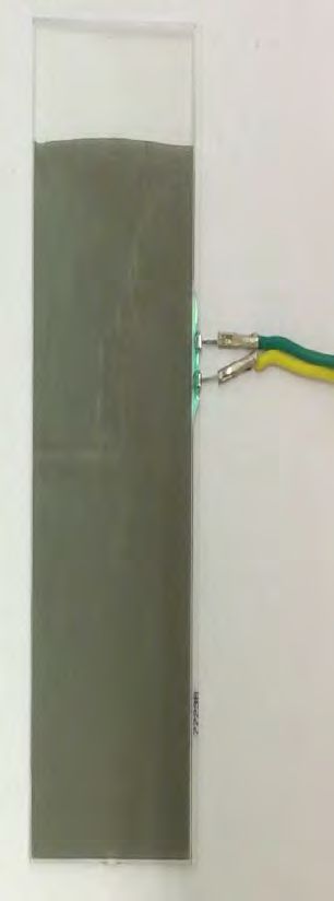
State of the
                  Liquid                Polarized White Light             Received Color with Polarizing Film at Different Angles
                                                                                                                                                           30
               Crystal Layer                                                                                                                                                                        w/o dispersion
                                                                                                                                                                                                    with dispersion

                                                                                                                                   Effective Intensity Diff (dB)
     w/o           ON                                                                                                                                      25
  Dispersion

                                                                                                                                                           20
                   OFF

                                                                                                                                                           15
               State of the                                 Colors in
                                Polarized
                  Liquid                     Dispersor      Different      Received Color with Polarizing Film at Different Angles
               Crystal Layer   White Light                                                                                                                 10
                                                           Polarization

     with          ON                                                                                                                                              5
  Dispersion

                                                                                                                                                                   0
                                                                                                                                                                    0   20   40   60   80   100   120   140   160     180
                   OFF                                                                                                                                                  Receiver’s orientation θ (degree)

                         Propagation Direction of the Back Light

Figure 5: Comparison between BCSK (w/ dispersion) and BISK (w/o dispersion). In BISK as in the upper sub-figure, the captured
white light in receiving camera can only be quantified using light intensity. In BCSK as in the lower sub-figure, a dispersor is added in
the VLC transmitter, the captured chromatic light can be quantified using a vector in RGB domain (i.e. color). The right sub-figure
shows in BISK, intensity-diff of two encoded states largely fluctuates with receiver’s orientation, whereas in BCSK, the effective
intensity-diff is stable.

tion. We also verified the result using experiments, in the angle of                                 on the liquid crystal layer, the color of the captured light changes as
45◦ , the intensity-diff is indeed very low.                                                         well. Although the captured color still differs with the orientation
   A possible solution is to ask users to rotate the receiving devices.                              of the receiving device, with proper dispersion we can guarantee
However, we believe it would be a cumbersome task. Since the                                         the received colors largely differ between two encoded states in any
polarizing angle is not perceivable by eyes, there is hardly any in-                                 orientation.
formation to guide users on how to rotate. Also, rotating wearable                                      Next, we describe how to tune the dispersion for the purpose of
devices could require big weird gestures.                                                            guaranteeing a reliable SNR in all orientations.
   To tackle this problem, we exploit the camera’s capability of tak-
ing chromatic video. Recall the rainbow, the white light consists                                     3.1.2        Tuning Dispersion and Optimizing SNR
of multiple colors of light. The basic idea is to disperse the polar-
                                                                                                         Dispersion tuning is performed by choosing the best thickness for
ized light emitted from the liquid crystal layer into different colors,
                                                                                                      disperor. The best thickness is mainly determined by the substance
so that the receiving camera can capture different colors in differ-
                                                                                                      of dispersor. The spectrum of the illuminating light may slightly
ent orientations after the filtering of the receiving polarizer. We
                                                                                                      affect the best thickness, but this effect is very small because most
fine tune the color dispersion to guarantee that, in any orientation,
                                                                                                      illuminating light sources emit white light which represents a sim-
the captured colors in two encoded states will be largely different.
                                                                                                      ilar flat spectrum. When the substance of dispersor and the type of
We term this color-based modulation as Binary Color Shift Keying
                                                                                                      light is determined, the best thickness is also determined.
(BCSK). Next, we describe the dispersor and BCSK in details.
                                                                                                         The target we optimize for is a metric called effective intensity-
                                                                                                      diff. It quantifies the color difference between two encoded states
3.1.1      Dispersor and BCSK                                                                         which is measured by camera. Therefore, it represents the received
   Some materials have a property called optical rotatory disper-                                     signal strength of the communication channel. Specifically, as shown
sion (ORD), i.e. they can rotate the light’s polarization differently                                 in Figure 6, the colors captured by camera are mapped into a {Red,
with different frequencies (colors) of light [10]. These substances                                   Green, Blue} (RGB) space. Given certain receiver orientation, the
may be solid such as quartz, liquid such as alcohol or gas such as                                    two colors in two encoded states can be indicated using two vec-
Hexadiene. This property has been studied for decades and widely                                      tors s~1 and s~2 . The difference between two colors is therefore
used in industry, chemistry and optical mineralogy. For example,                                     ~δ = s~1 − s~2 . Then, effective intensity-diff is defined as |~δ|.
the method for measuring the blood sugar concentration in diabetic                                       We formulize the optimization problem and solve the best thick-
people is based on the ORD property of the sugar. In this paper, we                                   ness Lbest as follows.
use a liquid substance called Cholest [13] as our dispersor for the                                      When a beam of polarized light passes through a dispersor, it
ease of fine-tuning the thickness and dispersion.                                                     is dispersed into multiple beams of polarized light in which each
   We use Figure 5 to illustrate BCSK by comparing it with Binary                                     has a unique frequency (color). The polarization of a beam with
Intensity Shift Keying (BISK). We can see the beam of the polar-                                      frequency f is rotated by an angle ∆φf , which is determined by:
ized white light emitted from the liquid crystal is dispersed into
multiple beams of polarized light with each having a unique color                                                                                       ∆φf = n(f )L,                                                 (2)
and polarization. The receiving polarizer passes through one beam
of light according to its polarizing direction and filters out other                                 where L is the thickness of dispersor, n(f ) is a function of f which
beams. Therefore, only a certain color is captured by the receiving                                  describes the rotation of light polarization in a unit thickness. n(f )
camera. When the encoded state is changed by the control voltage                                     describes the property of a substance.
180

                                                                              Minimum Effective Intensity Diff
                                    Green                                                                        160
                                                                                                                              Fluorescent
                                                                                                                              Solar
                                                                                                                 140          LED
                                                                                                                              Incandescent
                                                                                                                 120

                                                                                                                 100

                                                                    Blue
                                                                                                                  80

                                                                                                                  60

                                                                                                                  40

      Red                                                    −                                                    20

                                                                                                                   0
                                                                                                                    0                                                    1
                                                                                                                                       Nomailized Thickness

                         Figure 6: Effective Intensity-diff |~δ|.           Figure 8: The optimal thickness of dispersor is almost the same
                                                                            with various types of illuminating light, as most illuminating
   1D Sample Value

                                                                            light is white light.

                                                                                                                    Video
                                                                                                                   Preview

                                                                                                                   Beacon         3D(RGB)     Dimension     1D       Down
                                                                     Time                                         Detection       Samples     Reduction   Samples   Sampling

Figure 7: Result of dimension reduction. These 1D samples
reduced from 3D samples in Figure 6 constitute the received
waveform.                                                                                           CRC                          Packet       bits                    symbols
                                                                                                                                                       Demapping
                                                                                                   Check                        Detection
  After the filtering by the receiving polarizer, the light captured
by camera is described with a vector {IR , IG , IB } in RGB space.                         Beacon
{IR , IG , IB } can be derived using the Malus’ law:                                         ID                                                      BCSK Demodulation
               Z fmax
IN (θ, L) =            pN (f ) cos2 (n(f )L − θ) df, N ∈ {R, G, B}
                         fmin                                                                                          Figure 9: Structure of PIXEL’s VLC receiver.
where θ is the polarizing angle between transmitter’s polarizer and
receiver’s polarizer. fmin and fmax are the upper/lower frequency           it is because most illuminating light sources emit white light which
bounds of the light’s spectrum. pN (f ) describes the light spectrum        has a similar flat spectrum.
projected on the dimention N of RGB space. pN (f ) is determined                To compare BCSK with BICK, we calculate the effective intensity-
by the camera’s chromatic sensor. From this formula, we can ob-             diff under Lbest in all possible receiver orientation (represented by
serve that the light captured by camera is determined by both optical       θ). Results are shown in the rightmost of Figure 5. We can see the
rotatory dispersion (n(f )L) of the substance and the light spectrum        effective intensity-diff is quite stable in all the receiver orientations.
(pN (f )), as mentioned above.                                                  To conclude, the dispersor in PIXEL’s VLC transmitter and the
   The final goal of the optimization problem is to maximize the            color-based modulation scheme BCSK well solve the problem of
minimal effective intensity-diff in all receiving orientations. Con-        varying SNR caused by users’ mobility.
sidering the two encoded states between which the polarizing angle
is rotated by 90◦ , we can formulize the optimization problem as            3.2                                   VLC Receiver
follows:                                                                       PIXEL’s VLC receiver decodes beacon’s identity from camera’s
                   s      X                                     2          video preview. Figure 9 shows the structure of the VLC receiver.
    arg max min                    IN (θ, L) − IN (θ + 90◦ , L)                The first step is beacon detection. In order to save computation,
                     L   θ
                                N ∈{R,G,B}                                  we first downsample the video to contain less pixels. According
                                                                            to our experience, 100 × 100 pixels will be sufficient for decoding
   To solve this problem and get Lbest , we need to know n(f ) and          in a distance within 10 meters. Then we calculate the difference
pN (f ) in advance. n(f ) and pN (f ) can be obtained from speci-           between every two consecutive frames to detect the VLP beacons.
fication or calibration. In our work, we calibrate the n(f ) of our         In order to make the detection reliable, we add up the differences
dispersor by ourselves and derive pN (f ) from specification [8] and        from 10 consecutive frames. Usually a detected beacon contains 10
calibration results in literature [2]. We found pN (f ) almost does         or more pixels which contain its color value. We finally average
not affect the vlaue of Lbest , as shown in Figure 85 . We believe that     these pixels to generate a 3-dimensional ({R, G, B}) color sample
5
  We use the normalized thickness to plot the trend for dispersors          Length “1” means the the difference of the rotated angles between
with different materials. Given the condition that the n(f ) is ap-         fmin and fmax is 180◦ : |∆fmax − ∆fmin | = 180◦ and length “0”
proximately linearly related to f , the trend of the Figure holds.          means no difference in rotation, i.e. L=0.
120
Color difference mapped to 1D
100 Samples:
80
Symbol: 0 1 0
60
OS Time:
40
as
20 Downsampling point
0 20 40 60 80 100 120 140
OS Time mod 2 Symbol Periods (Second)
Figure 10: 3000 video samples overlay with their sampling
timestamp mod two symbol periods. The eye patten indicates
the clock drift between the OS clock and VLC transmitter is as
Downsampling point
negligible.
from every video frame. Once a beacon is detected, one frame with-
out downsampling is buffered for calculating its image location for
the localization algorithm in §3.3. as
As illustrated in Figure 6, these 3D samples in {R, G, B} space Downsampling point
are mainly distributed around two points, which represent the two
encoded states. Since there are only two points/states, for the ease
of further processing, we perform dimension reduction to convert
3D samples into 1-dimensional samples as the first step of BCSK Figure 11: Downsampling example on real samples. Each T0j
demodulation. The requirement of dimension reduction is to pre- determines a sampling sequence, PIXEL chooses T01 since it has
serve the distance between samples of the two encoded states. There- the best decoding SNR.
fore, we perform reduction by projecting these 3D samples to the
light. Moreover, the sampling rate may even vary during a single
difference vector between the two states, i.e. ~δ in Figure 6. The
video recording.
projection from a 3D sample ~s to 1D sample s is calculated by:
In PIXEL, we leverage the device’s OS clock to perform down-
~s · ~δ sampling. The core observation is that the clock drift between the
s= , (3) receivers’ operating system and the transmitter is negligible in the
|~δ|
time scale of several packet durations (seconds). This can be proven
Figure 7 shows the 1D sample waveform reduced from 3D samples by Figure 11, where every sample is timestamped by the OS clock
in Figure 6. To determine ~δ, we calculate difference vectors be- and plotted with the time modulo of two symbol intervals. The
tween every two consecutive 3D samples, then take the average of cross lines between the upper line and the lower line in the figure
those difference vectors with large norm and right direction as ~δ. are the boundary of the symbols. When there is a clock drift be-
In PIXEL’s transmitter, we set the symbol rate roughly the half of tween two clocks, the boundary will keeps moving. However, as
the camera’s sampling rate for the purpose of meeting the sampling we can see from the figure, the clock drift can hardly be observed.
theorem. As the low cost cameras in wearables are not stable in the We downsample the uneven samples according to the OS clock.
sampling interval, the downsampling process is non-trivial and we Although the sampling interval is changing, the relative optimal
will elaborate on it in §3.2.1. sampling time in one symbol period is stable. In Figure 10, sam-
The output of the downsampling module is symbols. Since the ples around 60 can achieve higher SNR than those close the symbol
symbols are in 1 dimension (scalar), demapping is equivalent to bit boundary. In order to find the optimal sampling time, we use a
arbitration which determines ‘1’ or ‘0’ from every symbol. Similar method similar as searching. Several candidates of the sampling
to classic 1-bit arbitrator designs, we set the average of all symbols time are used to downsample the incoming wave simultaneously,
as the threshold. and the best candidate in SNR gains weight in being the final choice.
The final step is to recover packets from the bit stream. In PIXEL, We choose the candidate which has the largest cumulative weight as
we use a 5-bit header for packet detection and synchronization. our sampling time for this symbol period. Note that the algorithm
Since the packet is short, we use a 4-bit CRC for error detection and can automatically adapt to different start conditions and bootstrap
do not perform channel coding or forward error correction. More the sampling time to the optimal choice. Once the sampling time is
details about the packet design is shown in §4. determined, we choose the nearest input point as the downsampling
result.
3.2.1 Combating the uneven camera sampling We explain the detailed downsampling method through Figure
The downsampling (decimation) algorithm in classic digital sig- 11. PIXEL maintains sampling candidates Tkj with same time in-
nal processing [30] cannot be applied to PIXEL’s VLC receiver. terval: Tkj = T0 + kC + jC/N, k ∈ N, j ∈ {1, .., N }, where k
A basic assumption behind these algorithms is that digital samples represents different symbol period and j represents the incremen-
are taken with a constant interval from the analog signal. However, tal searching step within one symbol period. C is the time for one
this assumption does not hold in the low-cost cameras. As [22] symbol period. Once T00 , for example, in the figure is selected as
pointed out, cameras in mobile devices do not offer fixed sampling the first sampling time, then Tk0 = T00 + kC is the correspond-
rate (frames per second). Specifically, the sampling rate differs on ing sampling sequence. According to the nearest rule, the selected
different cameras, and also differs under different levels of ambient samples for each T0j is shown in the bottom half of Figure 11. Ap-Algorithm 1 Adaptive Downsampling 2500 Levenberg−Marquardt algorithm
Input: Brute force search with 1cm grid size
N : The number of the sampling time candidates. 2000
Location Error (mm)
L: The length of historical samples used to calculate SNR.
k: The symbol period k.
1500
Tk1 ∼ TkN : Sampling time candidates at symbol period k.
tsi ∼ tsj : Timestamp of samples, tsi2.4m
Preamble Payload(Location ID) CRC
5bit 8bit 4bit
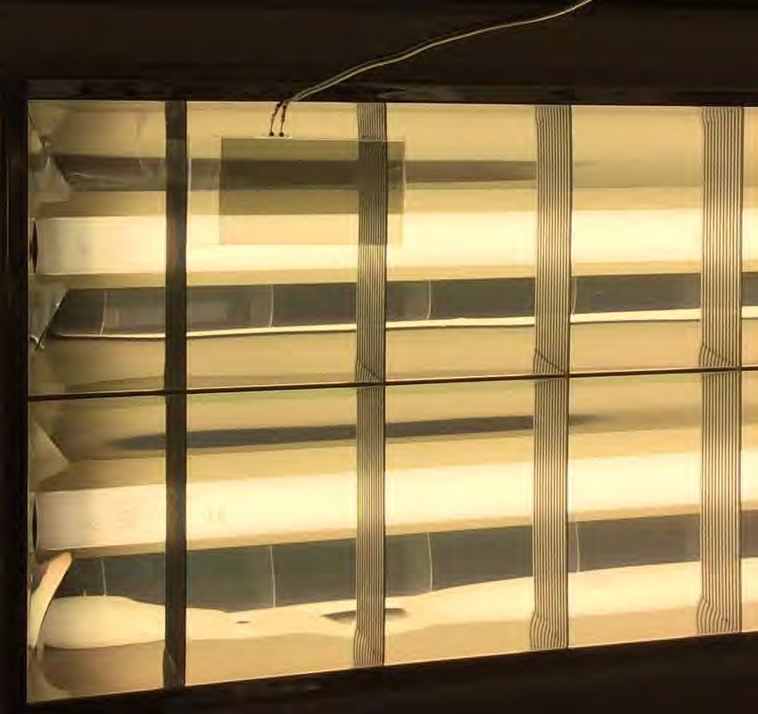
Figure 14: Message format of the location beacon. VLC 1.8m
Transmitter
VLC transmitter
VLC transmitter is (a) (b)
is attached to a
VLC transmitter Control Unit attached to an fluorescent lamp
LED Lamp
Figure 16: Evaluation Setting. (a) is the settings for single VLC
pair. d is the distance from the receiver to the transmitter. θ
Figure 15: Photos of PIXEL’s components. From left to right:
is the orientation of the camera. φ is the viewing angle of the
(1) VLC transmitter including a polarizing film, a liquid crystal
transmitter. (b) is the testbed for the VLP evaluation.
layer and a dispersor. (2) The control unit with Altera Cyclon 2
FPGA. (3) VLC transmitter attached to a LED lamp. (4) VLC
transmitter attached to a florescent lamp.
We implement the VLC decoding and the positioning algorithm
in both Android system and an offline simulator6 . The code can be
nents except the dispersor which are constructed using liquid and easily ported to other platforms since it does not depend on specific
transparent container. On the other side, we implement the VLC re- APIs. In Android 4.1.4, it takes 1200 lines of codes and the size of
ceiver and the positioning algorithm in a software program for both the executable file (apk) is about 320kb. We use the preview data
Android phones and Google glass. from the camera to process decoding in realtime. As the system will
automatically adjust camera’s exposure time according to the inten-
4.1 PIXEL’s Hardware sity of the received light, which may affect the BCSK decoding. We
One VLC transmitter consists of three transparent optical layers walk around this issue by manually locking the exposure time in
and one control unit. The first layer is a linear polarized film [6], the software. This is not an issue in new Android release [1], since
which functions as a polarizer to polarize the illuminating light. more flexible control of exposure time is provided. Once enough
The second layer consists of two pieces of glasses with liquid crys- beacon packets are received, we use the buffered video frame to
tal in between. We add electrodes on both glasses to control the calculate the locations of lamps in the image for the localization al-
applied voltage. This layer is a kind of simplified LCD with only gorithm. Other required parameters (i.e. the focal length of the lens
one pixel, and many LCD manufacturers have the service for cos- and the size of the image sensor) can either be read from the EXIF
tuming LCD [4]. The third layer is a dispersor. We prototype this stamp of the camera or obtained from online specifications.
layer by filling the optical rotation material (Cholest) into a glass
box. We choose the liquid material because it is easy to tune the 5. EVALUATION
thickness, but solid materials [7] with appropriate thickness could
be a good choice for the real deployment. We adopt Altera’s Cy- In this section, we evaluate PIXEL’s design based our prototype
clone II FPGA to control the voltage of the liquid crystal layer. Its implementation. We first describe the evaluation setup, then we
clock rate is 40MHz and the output voltage is 0V/3.3V. The two conduct experiments to verify the component design in PIXEL. Af-
electrodes of the liquid crystal layer are directly connected to two ter that, we thoroughly evaluate different impact factors on PIXEL’s
output ports of the FPGA to modulate the light’s polarization. VLC subsystem and the computational cost of each part of the client
Each PIXEL’s transmitter works independently by facing to nor- application. Lastly, we present the overall performance of our VLP
mal light sources such as solar light, LED light, fluorescent light system.
and so on. As Figure 15 shows, normal light sources can thus be
easily upgraded to have VLC ability with PIXEL’s transmitter de-
5.1 Experiment Setting
sign. Evaluation involving one single pair of transmitter and receiver is
The hardware of PIXEL’s client devices requires no modification performed in controlled conditions. Figure 16 (a) shows controlled
or customized accessories. The only requirement is a small piece parameters related to user’s mobility. d is the distance between the
of off-the-shelf linear polarizing film, and it is placed in front of the transmitter and the receiver. θ is the receiver’s orientation whose
camera to detect and receive VLC signals. rotation plane is parallel to the receiver’s plane. φ is the viewing an-
gle whose rotation plane is vertical to the transmitter’s plane. Other
4.2 PIXEL’s Software impact parameters such as the downsampled resolution7 and the ex-
The packet format of VLC is designed for the indoor localization posure time are also controlled in the evaluation. If not mentioned,
purpose. PIXEL’s transmitter continuously broadcasts its location we take d = 3m, θ = 0◦ , φ = 0◦ , downsampled resolution =
identity to receivers. The beacon packet contains a 5-bit preamble, 120 × 160 and exposure time = 1/100s as default settings.
an 8-bit data payload and a 4-bit CRC. The preamble is used for Evaluation involving multiple pairs of transmitter and receiver is
packet synchronization. Once the receiver detects a preamble from performed with the testbed in Figure 16 (b). We fix eight PIXEL’s
cross-correlation, it will start to decode the following packet pay- 6
load which contains the identity of the beacon. We choose 8-bit We extract Presentation Time Stamp (PTS) from ffmpeg [3] to
simulate timestamps of frames in recoded videos.
as the length of an identity by considering the lamp density of the 7
The downsampling is used to reduce processing overhead as we
real world deployment. For the 4-bit CRC, the probability of false- mentioned §3.2, we fix the downsampled resolution to certain val-
positive detection is only 1.7 × 10⁻⁸ [24] in our scenario, which is ues, such as 120 × 160. The reason is to normalize different reso-
small enough. lutions across cameras.w/o dispersion
1
30 with dispersion optimal
Effective Intensity Diff (dB)
with dispersion implemented
0.8
25
20 0.6
CDF
15 0.4 N=5
N=5 Optimal
10
0.2 N=3
5 N=15
0
0 14 16 18 20 22 24 26 28
0 20 40 60 80
Receiver’s orientation θ (degree)
100 120 140 160 180
SNR (dB)
Figure 17: Evaluation of the dispersor design Figure 18: SNR of adaptive downsampling. We choose the ap-
propriate number of searching candidates N = 5 in our design
to balance the accuracy and computational cost. Moreover, our
adaptive downsampling algorithm almost has the same perfor-
transmitters into a board which is elevated to the ceiling. The loca-
mance with the optimal downsampling choice.
tion of each transmitter is measured and mapped to the location ID
in client’s database. When the testbed is used for positioning evalu- 5.2.2 Adaptive Downsampling
ation, transmitters transmit their location ID through frame defined
Experiment: We evaluate the adaptive downsampling algorithm
in §14. Under the testbed, we grid another board to serve as ground
through real data and the offline processing. 65 logged cases are
truth reference for client’s location.
collected by receiving VLC data from different locations and ori-
We use controlled random bit stream for transmission to mea-
entations. Each log lasts for 30s. According to the logged color
sure BER and SNR. In these experiments, the transmitter repeat-
sequence and timestamps, we use offline simulator to adjust the
edly transmits a random pattern with a length of 100 bits, while the
number N of the potential choices of the sampling time. In each
receiver keeps logging the received color values and the decoded
choice of N , we calculate SNR for the whole sequence.
bits. Since the length of the random pattern is long enough, we
Results: Figure 18 shows the results. First, we compare the
determine the start of the transmitted pattern through correlation.
adaptive downsampling with the fixed downsampling, where a fixed
Therefore, the decoded bits can be used to calculate BER by com-
sampling time is chosen during the whole decoding. According to
paring with the known random pattern. With the known random
our previous description for Figure 10, the optimal choice of the
pattern as ground truth, the received color values can be used to
fixed sampling time is fixed but unknown. Adaptive downsampling
calculate SNR according to formula (4).
bootstraps and approximates such optimal choice. Figure 18 shows
All the experiments are done without a fixed ambient light source.
that when N = 5 the adaptive downsampling has little difference
In the morning, the ambient light is solar light and becomes fluo-
from the optimal choice of fixed sampling. We note that the same
rescent light in the evening. We adopt the 5W 10cm×10cm LED
conclusion holds for different N , but we omit the curves for clarity.
lamp as the light source of the transmitter for convenient setup. We
Second, we study the trend of the decoding SNR when N in-
also have performed similar evaluation experiments for fluorescent
creases. Reasonably, the SNR curve of larger N is better. This is
light and solar light, but we found little difference from LED.
simply because the choice for sampling time is more fine-grained
and flexible with larger N . However, the gain is bounded by the
5.2 Visible Light Communication intrinsic noise in the sampling timestamp and the communication
channel. Therefore, the SNR gain from N = 3 to N = 5 is
5.2.1 Dispersor and BCSK more significant than the gain from N = 5 to N = 15, and the
Experiment: We study the effectiveness of the dispersor design gain is even smaller when N is increased to larger values. Accord-
in PIXEL. The evaluation is taken in a static situation, i.e. the trans- ing to the measurement of our receivers, the standard derivation
mitter stops transmitting and is either in on or off stage. At each of the sampling time is in 6ms level. So we choose N = 5, i.e.
stage, we take pictures of the light in different orientations from 0◦ 1s/14/5 = 14ms, to bound the random timing error. Other de-
to 360◦ in step of 10◦ . From the two pictures at the same angle but vices can easily obtain appropriate N according to their local mea-
different stages, we compute the effective intensity diff according surement.
to the extract color of the light.
Results: The lined dot in Figure 17 shows the effective intensity 5.2.3 End-to-End Communication
diff of our dispersor prototype. Results from 180◦ to 360◦ are sym- Experiment: We study PIXEL’s VLC subsystem against five im-
metrical to 180◦ to 0◦ and omitted. Compared with the dash line, pacting factors caused by user mobility and device diversity: the
which is the results without the dispersor, the dispersor design sig- distance d, the receiver’s orientation θ, the viewing angle φ, the
nificantly increases the detectable difference for the on/off stages in downsampled resolution and the exposure time of the camera. The
degrees around 45◦ . Compared to the solid line, which is the situa- experiment for certain factor varies that factor to all the reasonable
tion with theoretical optimal dispersor design, our current prototype values, and fixes other factors.
can be improved. The reason is not the hardness for manufacturing Results: Figure 19 (a) shows the SNR against the distance and
the dispersor, but lies in the fact that we can only purchase glass the downsampled resolution. The downsampled resolution and the
boxes with fixed thickness in the market. We choose the best exist- distance determine the number of pixels of the transmitter in the
ing thickness to prototype and we believe its performance is enough received image, and thus affect the SNR in a similar way. There-
to illustrate our design. fore, we list them in the same figure for better illustration. From
the results, our system achieves the SNR higher than 15dB under
120 × 160 resolution within 13m, which is sufficient for most in-30 30
30 w/o dispersion
120*160 with dispersion
60*80 25 25
25
30*40
20 20
20
SNR (dB)
SNR (dB)
SNR (dB)
15 15
15
10 10
10
5
5 5
0 0 0
1 2 3 4 5 6 7 8 9 10 11 12 13 0 20 40 60 80 100 120 140 160 180 −80 −60 −40 −20 0 20 40 60 80
Distance (m) Receiver’s orientation θ (degree) Viewing Angle (degree)
(a) SNR v.s. distance and resolution (b) SNR v.s. orientation (c) SNR v.s. viewing angle
30 10
0 60
Measured
25 Theoretical 50
Throughput (bps)
20 10
−1 40
SNR (dB)
BER
15 30
10 10
−2 20
5 10
0 10
−3 0
1/30 1/300 1/800 1/1800 1/3300 0 5 10 15 20 25 30 1 2 3 4 5 6 7 8
Exposure Time (s) SNR (dB) Number of PIXEL
(d) SNR v.s. exposure time (e) BER v.s. SNR (f) Rate v.s. number of PIXEL
Figure 19: PIXEL communication evaluation
door localization scenarios. In addition to that, the VLC system the glow of the transmitter’s image. Therefore, our VLC is robust
works even when the downsampled resolution is as low as 30 × 40. under different exposure settings.
Notice that the SNR of the downsampled resolution of 60 × 80 and Figure 19(e) summarizes the data from all the experiments and
30 × 40 drops to 0 at 13m and 7m respectively. The reason is that get the relationship between BER and SNR. The theoretical curve
our decoding algorithm needs enough pixels to extract color. How- for BCSK is calculated according to BPSK. However, since the
ever, when the distance from the transmitter increases, the transmit- camera of our smartphone is not stable enough and may occasion-
ter’s pixels in the image decrease. This is not a problem since even ally drop frames during the capturing, the bit error rate is slightly
13m is enough for VLP in a normal building. Moreover, the size higher than the theoretical result. Another reason is the number of
of the transmitter or the intensity of the background light can easily samples for statistics is not enough. It can be observed from the
be increased to satisfy the possible requirement. two “horizontal lines” in the bottom of the Figure 19(e). Since each
Figure 19(b) shows the VLC performance under different ori- logged data only contains hundreds of bits on average, the upper
entations. Without the dispersor, the SNR becomes undecodable “line” is plotted by cases with 2 error bits and the other “line” is
when the view angle between the transmitter and receiver is around formed by cases with 1 error bit.
40◦ or 130◦ . This result is in accord with our previous analysis Figure 19(f) shows the VLC throughput versus the number of
about effective intensity diff in §5.2.1. On the other hand, the result transmitters. The rate is counted by the received payload, which
is improved a lot when the dispersor is deployed. The SNR of the does not contain the preamble and CRC. The result shows that the
received data is around 16dB in all the orientations, implying that throughput increases linearly with the number of transmitters. It im-
the VLC quality is stable despite different orientations. plies that concurrent transmissions don’t affect the performance of
Figure 19(c) implies that the performance of VLC is stable under our VLC. This is reasonable, since each transmitter is independent
different viewing angles from −60◦ to 60◦ , which is sufficient for and the decoding process for each transmitter is also independent.
normal localization scenarios. From the results, we also observe
that the variance of the SNR in the positive and negative sides are
asymmetric. This is caused by the viewing angle limitation of the
5.3 Visible Light Based Positioning
prototyping TN LCD, and can be solved by using better TN LCD
or other LCD such as In-Plane Switching LCD. 5.3.1 Computational Cost
Figure 19(d) shows the SNR against different exposure time set-
Experiment: We study the computational cost of PIXEL’s client
tings of the camera. The result implies that there is no obvious re-
application in detail. The evaluation is performed with Samsung
lationship between exposure time and SNR. The reason is that our
Galaxy SII. Its CPU has dual cores with maximum frequency of
decoding algorithm will use different areas for decoding according
1200 MHz. We fix the frequency to 1200 MHz though an app
to the exposure time. When under short exposure time, the amount
SetCPU. It has two cameras and we use the back one with 8 Megapixel
of the received light from the transmitter is small and the decoding
for this evaluation. The smartphone is fixed in one location to per-
algorithm uses the center part of transmitter to extract color. When
form VLP and its distance to the testbed in Figure 16(b) is 3m. We
under long exposure time, the center of the transmitter is overex-
log the start and end time exclude the sleep period in each part of
posed and displays white. However, the color can be extracted from
our program to calculate the processing time. This method may be
affected by the CPU scheduling, so we close all the other applica-200
VLC Processing time per packet (ms)
60 5
VLC Processing time per packet (ms)
Proccesing Time for Positioning(ms)
50
4
150
40
3
30 100
2
20
50
10 1
0 0
240*320 120*160 60*80 0
1 2 3 4 5 6 7 8 3 4 5 6 7 8
Resolution(pixel*pixel) Number of PIXEL
Number of PIXEL
(a) Processing time for VLC v.s. resolution (b) Processing time for VLC v.s. number of(c) Processing time for localization algo-
PIXEL rithm v.s. number of PIXEL
Figure 20: Computational cost of each component
1 1 1
0.8 0.8 0.8
0.6 0.6 0.6
CDF
0.4 0.4 0.4
Google Glass 300MHz
Google Glass 600MHz
0.2 0.2 0.2 Google Glass 800MHz
Samsung Galaxy S2 1200MHz
0 0 0
1 1.5 2 2.5 0 50 100 150 200 250 300 350 400 450 0 50 100 150 200 250
Positioning Delay (s) Postioning Error (mm) Positioning Time Cost (ms)
(a) Positioning Delay (b) Positioning Error (c) Processing time of VLP
Figure 21: VLP overall performance
tions and unnecessary services in the smartphone to keep the results bitrary orientations and ensure that at least 3 transmitters can be
as accurate as possible. captured by the camera. The start time and the end time of each test
Results: Figure 20(a) shows the computational cost under differ- are logged for delay analysis. The localization results and the cor-
ent resolutions with single transmitter. Each packet is 17 bits and responding ground truth are recorded to estimate localization error.
takes 1200ms air time for transmitting, but our decoding algorithm Like previous subsection, we log the processing time of the appli-
costs less than 50ms even when the resolution is 240 × 320. The cation to analyze the overhead. Since Google Glass has different
result indicates our decoding algorithm performs fast enough. The frequency settings, we traversal all the configurations in our tests.
figure also shows that it takes less time for processing when the Results: Figure 21(a) shows that the average time from the launch
downsampled resolution is lower. This is intuitive, because it takes of the application to a successful positioning is about 1.8s. It is
less pixels for processing color extraction. reasonable, because the time from the launch of the application to
Figure 20(b) shows the time cost when the client is receiving the earliest arrival of the beacon packet is uniformly distributed be-
from multiple transmitters. It shows that the total time of decoding tween 0 and 1200ms. Figure 21(b) shows the localization error is
8 concurrent packets is less than 200ms, which is still far less than less than 300mm in 90% test cases. The accuracy is in accord with
the packet air time 1200ms. The trend shows the decoding time in- existing results [25]. Figure 21(c) shows the CDF of the computa-
creases linearly with the number of transmitters. This is because the tional cost under different CPU settings. As mentioned above, the
decoding process for each transmitter is independent and scalable. computational cost includes the VLC decoding and the localization
We also note that the 8 cases share a small portion of basic process- algorithm. Even with a limited processing ability such as 300MHz,
ing cost, which is actually contributed by the shared downsampling our design can finish all the calculation within 150ms on average,
process. which is still far less than the transmission time of one location
Figure 20(c) shows the time cost of the localization algorithm. beacon (1200ms). Therefore, the results validate that PIXEL can
Since it requires at least 3 anchors, the number of transmitters starts provide smart devices with light-weight and accurate localization
from 3. The result demonstrates that the localization can be fin- ability.
ished within 5ms after the client receives enough beacons. The
processing time slightly increases with the number of anchors, this 6. RELATED WORK
is caused by the increased dimension in the object function.
Visible Light Communication. VLC has been studied with dif-
ferent context and design goals. Comparing with radio communi-
5.3.2 VLP Performance cation using microwave or mmwave, VLC uses visible light which
Experiment: We study the overall VLP performance of PIXEL has much higher frequency and much wider bandwidth. Typical
in three aspects: positioning delay, positioning error and position- VLC research aims to provide very high link throughput commu-
ing overhead. We use Samsung Galaxy SII and Google Glass as nication [23] for the purpose of wireless access [33]. Normally the
client devices while the transmitters in Figure 16(b) serve as VLP receiver requires a photodiode to receive the modulated light. Dif-
anchors. We place client devices to 100 random locations with ar- ferent from this goal, our design focuses on providing a light-weightYou can also read