A spectral approach to estimating the timescale-dependent uncertainty of paleoclimate records - Part 2: Application and interpretation
←
→
Page content transcription
If your browser does not render page correctly, please read the page content below
Clim. Past, 17, 825–841, 2021
https://doi.org/10.5194/cp-17-825-2021
© Author(s) 2021. This work is distributed under
the Creative Commons Attribution 4.0 License.

A spectral approach to estimating the timescale-dependent
uncertainty of paleoclimate records – Part 2: Application
and interpretation
Andrew M. Dolman1 , Torben Kunz1 , Jeroen Groeneveld1,2 , and Thomas Laepple1,3,4
1 Alfred-Wegener-Institut Helmholtz-Zentrum für Polar- und Meeresforschung, Research Unit Potsdam,
Telegrafenberg A45, Potsdam, 14473, Germany
2 Institute of Geology, Hamburg University, 20146 Hamburg, Germany
3 Department of Geosciences, University of Bremen, 28359 Bremen, Germany
4 MARUM – Center for Marine Environmental Sciences and Faculty

of Geosciences, University of Bremen, Bremen, 28334, Germany

Correspondence: Andrew M. Dolman (andrew.dolman@awi.de)

Received: 18 December 2019 – Discussion started: 13 February 2020
Revised: 13 November 2020 – Accepted: 10 February 2021 – Published: 8 April 2021

Abstract. Proxy climate records are an invaluable source of        1   Introduction
information about the earth’s climate prior to the instrumen-
tal record. The temporal and spatial coverage of records con-      Proxies of climate variables, such as geochemical indicators
tinues to increase; however, these records of past climate are     of temperature in marine sediments or ice cores, are a valu-
associated with significant uncertainties due to non-climate       able source of information about the earth’s climate prior to
processes that influence the recorded and measured proxy           the instrumental record. However, these records are an imper-
values. Generally, these uncertainties are timescale depen-        fect representation of past climate as they are also influenced
dent and correlated in time. Accounting for structure in the       by non-climatic factors in addition to the climate signal. Er-
errors is essential for providing realistic error estimates for    rors in a proxy record mean that the past climate inferred
smoothed or stacked records, detecting anomalies, and iden-        from these proxy records is uncertain; understanding these
tifying trends, but this structure is seldom accounted for. In     associated uncertainties is important for all quantitative uses
the first of these companion articles, we outlined a theoretical   of climate proxies, such as data assimilation (Goosse et al.,
framework for handling proxy uncertainties by deriving the         2006), model–data comparisons (Lohmann et al., 2013), hy-
power spectrum of proxy error components from which it is          pothesis testing (Hargreaves et al., 2011), and the optimal
possible to obtain timescale-dependent error estimates. Here       combination and synthesis of climate records (Marcott et al.,
in Part 2, we demonstrate the practical application of this        2013; Shakun et al., 2012). Finally, knowing the error as a
theoretical framework using the example of marine sediment         function of environmental or proxy-specific parameters also
cores. We consider how to obtain estimates for the required        allows for the optimization of the sampling and measurement
parameters and give examples of the application of this ap-        strategy in order to obtain the information required to test
proach for typical marine sediment proxy records. Our new          specific hypotheses.
approach of estimating and providing timescale-dependent              Errors in a proxy record, defined here as differences be-
proxy errors overcomes the limitations of simplistic single-       tween the climate inferred from the proxy record and the
value error estimates. We aim to provide the conceptual basis      true climate, are introduced at multiple stages between the
for a more quantitative use of paleo-records for applications      true climate signal and final inferred past climate time series
such as model–data comparison, regional and global synthe-         (see, for example, Evans et al., 2013; Dee et al., 2015; Dol-
sis of past climate states, and data assimilation.                 man and Laepple, 2018). Importantly, the resulting errors are
                                                                   not all independent in time, rather they are often correlated

Published by Copernicus Publications on behalf of the European Geosciences Union.
826                                                            A. M. Dolman et al.: Timescale-dependent uncertainty – Part 2

and timescale dependent (Fig. 1). Currently the temporal co-       2     Error spectra as a framework for
variance structure of proxy uncertainties is largely ignored             timescale-dependent proxy uncertainty
in the literature (but see Moberg and Brattström, 2011). In
many cases, a single number, perhaps derived from a cal-           In this section, we illustrate the error spectrum framework
ibration data set, is reported as the uncertainty for a given      for the specific example of temperature-related proxies in the
proxy. However, its utility is very limited without additional     shells of planktic foraminifera recovered from marine sedi-
information about the structure of the error. For example,         ment cores. The major processes contributing uncertainty to
consider an error of 1.5 ◦ C. If the error were due to an un-      these proxy records have been explored using physically mo-
certainty in the temperature to proxy relationship, e.g., the      tivated proxy forward models that simulate pseudo-proxies
error of the intercept of a linear calibration equation, the       from an assumed true input climate (Laepple and Huybers,
uncertainty of a time slice containing multiple observations       2013; Dolman and Laepple, 2018). These processes include
would still be 1.5 ◦ C as the error does not reduce by av-         seasonality in the creation of proxy signal carriers (e.g.,
eraging more samples calibrated using the same equation            foraminiferal tests), aliasing due to under-sampling of the
(Fig. 1c), while the error from calibration on a difference be-    seasonal climate cycle, mixing and smoothing of the signal
tween two time slices would be zero. On the other hand, if         due to bioturbation, and independent measurement and pro-
this error were independent in time and thus between sam-          cessing error. One approach to estimating the uncertainty for
ples, e.g., if it were related to the error of a measurement       a given metric and proxy record is to use such a forward
device, the uncertainty of √a time slice based on nine samples     model to simulate ensembles of pseudo-proxy records, cal-
would be just (1.5 ◦ C / 9) = 0.5 ◦ C, while the error in the      culate the metric for each, and then examine their statistical
difference
         p between two time slices would be approximately          properties. In the approach we propose here, we do not sim-
0.7 ◦ C ( 2 · 0.52 ). Indeed, a number of recent studies assume    ulate pseudo-proxies for a specific climate time series, rather
independence in time (and space) and thus arrive at unrealis-      we make some simplifying assumptions about the properties
tic uncertainty estimates (e.g., Fedorov et al., 2013; Shakun      of the power spectrum of the climate and then estimate the
et al., 2012; Marcott et al., 2013).                               uncertainty directly from expressions for the power spectra
   More difficult than either fully independent errors             of the errors associated with proxy creation. The advantage
(Fig. 1a), or constant errors or “biases” (Fig. 1c), are cor-      of this analytical method over simulation is that it allows
related errors that manifest as slowly varying biases (Fig. 1b)    for very rapid assessments of proxy error, the relative con-
for which we need to quantify both the magnitude and auto-         tribution of different error sources, and the expected corre-
correlation structure. The idea we introduce in Part 1 (Kunz       lation between replicated proxy records and between proxy
et al., 2020) is to work in the spectral domain as this al-        records and the true climate – and all of these at multiple
lows for an explicit representation of the timescale depen-        timescales. This makes it possible to scan potential coring lo-
dence of uncertainty. Assuming a stationary climate process,       cations, to develop sampling and measurement strategies to
the power spectrum of a proxy error contains all the infor-        optimize future data acquisition, and to help interpret exist-
mation required to derive timescale-dependent uncertainties,       ing records. Finally, PSEM also provides a basis for estimat-
and working in the frequency domain further simplifies the         ing the spectrum of climate variability from error-corrupted
estimation of the different error components. A number of          proxy records at a future stage.
additional useful quantities, such as the uncertainty in a time-
slice mean, the uncertainty in the difference between two
time slices, and the expected timescale-dependent correla-         2.1    A simple model for the power spectrum of the
tion between replicates of proxy records and between proxy                climate
records and the true climate, can easily be derived from the
error spectrum.                                                    The uncertainty from some proxy error sources depends on
   In Part 1, we discuss the theoretical basis for and give        the strength of the variations in the climate. For example, the
a full mathematical derivation of the Proxy Spectral Error         error from smoothing a time series is zero if the time series is
Model (PSEM). Here in Part 2, we aim to facilitate the use         constant and becomes larger the more the time series varies.
of PSEM in paleoclimate applications. Thus, we (1) sketch          We therefore need a model for the variability of the climate,
the concepts behind the different error components in a more       and we describe this using the power spectrum of the cli-
applied way, (2) provide heuristic approaches to parametrize       mate S(ν) (see Sects. 2.1 and 3.1 of Part 1). While the devel-
the climate spectra and other parameters of the error model,       oped approach allows for any choice of a climate spectrum,
(3) provide examples using virtual and actual sediment cores,      e.g., from complex climate models or estimated from obser-
and (4) provide an R package implementing the spectral error       vations, we here outline a heuristic method suitable for ma-
estimation method.                                                 rine sea-surface temperature (SST) and surface δ 18 O calcite
                                                                   records. This method is implemented in the PSEM R package
                                                                   and requires only the core position and habitat depth range as
                                                                   input parameters.

Clim. Past, 17, 825–841, 2021                                                          https://doi.org/10.5194/cp-17-825-2021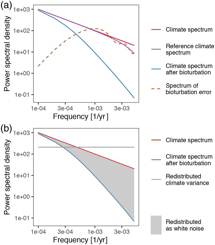
A. M. Dolman et al.: Timescale-dependent uncertainty – Part 2                                                                                 827

Figure 1. Illustration of different timescale dependences of proxy errors. The independent and correlated errors both have standard deviations
of 1.5 ◦ C, while the constant error is 1.5 ◦ C with zero standard deviation.

   A detailed, site-specific power spectrum of the climate
can only easily be estimated empirically for timescales up to
the length of the instrumental record. At longer timescales,
the climate spectrum can be approximated by a power-law-
type scaling, S(ν) = αν −β , where the exponent β charac-
terizes the scaling behavior and is thought to lie between 0
and 2 (Lovejoy, 2015; Schmitt et al., 1995), and α scales
the amplitude of climate variation. Here we take the prag-
matic approach of splicing zonally averaged empirical cli-
mate spectra for frequencies above 1/33 years with theo-
retical power-law spectra at lower frequencies (Laepple and
Huybers, 2014b) (Fig. 2). As the empirical spectra were esti-
mated from annual-resolution ocean temperature records, we
set power to zero at frequencies above 1/2 years.
   For the power-law section of the climate spectra, α was
chosen so that the low-frequency power-law spectra are con-                 Figure 2. An example spliced empirical and power-law power spec-
tinuous with the empirically estimated high-frequency re-                   trum of ocean temperature (0–120 m water depth) for 20◦ N latitude.
gions of the spectra. We typically assume a value of 1 for                  A small discontinuity at ν = 0.03 is visible, since to increase the ro-
β as this was found to be a good description of Holocene                    bustness of the intercept estimate, the splicing is implemented by
SST variability (Laepple and Huybers, 2014a), but this pa-                  matching the integrated spectra between ν = 0.03 and ν = 0.1.
rameter can be freely specified, and we illustrate the affect of
varying this parameter in Appendix A. To allow these spec-
tra to also be used for δ 18 O records, we recalibrate them to                 Additionally, the amplitude of earth’s seasonal tempera-
δ 18 O calcite units using a standard calibration (Bemis et al.,            ture cycle varies over a precessional orbital cycle with an
1998), which in terms of variance is effectively just a division            approximate frequency of 1/23 kyr. The magnitude of this
by a factor of 4.82 , assuming that the δ 18 Ocalcite is generally          amplitude modulation depends primarily on latitude, and we
dominated by temperature variations at these timescales. A                  assume this is equal to the amplitude modulation of incoming
function to generate these spliced empirical and power-law                  solar radiation at a given latitude (Berger and Loutre, 1991).
spectra is supplied as part of the PSEM R package.                          This introduces a low-frequency (1/23 kyr) deterministic sig-
   To this stochastic climate, we add a deterministic seasonal              nal to the climate.
cycle modeled as the power spectrum of a sine wave with a
frequency of 1/1 year (see Sect. 3.2 in Part 1). For a given
location, we parametrize the amplitude of the seasonal cy-                  2.2   Proxy error processes as filters
cle using a gridded data set of assimilated physically consis-
tent δ 18 Osw and temperature (Breitkreuz et al., 2018). The                During the creation of a climate proxy record, some of the
δ 18 Ocalcite value was calculated on the Pee Dee belemnite                 processes that introduce errors, defined here as differences
(PDB) scale from δ 18 Osw and temperature using the equa-                   between the proxy record and the true climate, can be thought
tions of Shackleton (1974).                                                 of as acting like filters on the true climate signal. Here we
                                                                            illustrate the concept of PSEM by considering the smoothing

https://doi.org/10.5194/cp-17-825-2021                                                                       Clim. Past, 17, 825–841, 2021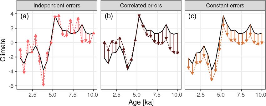
828                                                               A. M. Dolman et al.: Timescale-dependent uncertainty – Part 2

effects of bioturbation and the width of sediment slices from
which signal carriers, e.g., foraminiferal shells, are extracted.
   Bioturbation at the water–sediment interface mixes the up-
per few centimeters of sediment, thereby mixing together sig-
nal carriers of different ages. This acts like a smoothing filter
on the climate signal, reducing the amplitude of climate vari-
ations in a frequency-dependent way. The magnitude of the
reduction at each frequency depends on the filter characteris-
tics; using the simple physical bioturbation model of Berger
and Heath (Berger and Heath, 1968), the filter width, τb , is
simply the bioturbation depth divided by the sedimentation
rate. In the frequency domain, this is equivalent to multiply-
ing the power spectrum of the climate with the transfer func-
tion of the filter and results in a power spectrum of the error,
as described in Sects. 2.2 and 3.1 of Part 1.
   Similarly, when a sediment core is sampled, the proxy sig-
nal carriers are picked from a series of slices of sediment,
each with a finite width of typically 1–2 cm. This again acts
as a filter, this time a running mean filter with width, τs , equal
to the ratio of the slice thickness and sedimentation rate. As
for the bioturbation filter, in the frequency domain the effect
on the original signal is obtained by multiplying the power
spectrum with the transfer function of the filter (see Sects. 2.3
and 3.1 in Part 1).
                                                                      Figure 3. A conceptual representation of PSEM. (a) The true cli-
                                                                      mate signal is filtered (smoothed) by processes such as bioturba-
Error relative to the reference climate                               tion. This modifies the power spectrum of the climate (red) in a
                                                                      frequency-dependent way, producing the power spectrum of the cli-
So far we refer to a proxy error as a difference between the
                                                                      mate signal after bioturbation (blue). Proxy records are assumed to
measured proxy value and the “true” climate signal. The bio-
                                                                      represent the climate at a particular timescale (e.g., centennial, mil-
turbation and slice thickness filters smooth the climate signal       lennial), and the reference climate spectrum (purple) is the power
so that the proxy differs from the true climate. However, in          spectrum of the true climate smoothed to this timescale. The error
practice, values of proxy variables from marine sediments             that bioturbation and other smoothing produces (dashed brown) is
are rarely interpreted as representing the instantaneous cli-         a function of the reference and bioturbated climate spectra. (b) The
mate state; it is understood implicitly that some smoothing           power of the true climate signal that is removed by bioturbation
has taken place. The error therefore depends on the inter-            and other smoothing processes (gray shaded region) can be redis-
preted timescale of the proxy record, and so, in the spectral         tributed as a white noise error component (gray horizontal line) if
error model, we define error relative to the true climate at          the time period over which individual signal carriers are created
a specific timescale provided by the user (see Sect. 2.4 in           (e.g., foraminiferal tests calcify) is short relative to the timescale of
                                                                      the smoothing processes. This white noise term is reduced if multi-
Part 1). The power spectrum of this error is shown as the
                                                                      ple signal carriers are measured together or if their values are aver-
dashed brown line in Fig. 3a.
                                                                      aged together later.

2.3   Redistribution of climate power due to
      under-sampling

The proxy quantity (e.g., δ 18 O, Mg / Ca, etc.) is often mea-
sured on a finite number, N, of discrete signal carriers such
as foraminiferal tests, each of which calcifies and records or        error caused by the smoothing. The variance of this stochas-
samples a short snapshot of the climate, typically 2–4 weeks          tic error term is equal to the integral of the difference between
for pelagic foraminifera (Bijma et al., 1990; Spero, 1998).           the climate spectrum and the spectrum of the smoothed cli-
The bioturbation and slice thickness filters can be thought           mate signal divided by the number of individual signal car-
of as probability density functions (PDFs) that describe the          riers in a sample, shown as the gray line and shaded area in
portion of time from which the climate signal is sampled by           Fig. 3b (see Sects. 2.3 and 3.1 in Part 1). As N tends to infin-
these N signal carriers. As this is a finite sample, the result-      ity, the error due to under-sampling tends toward zero. This
ing proxy value is an estimate of the mean value and contains         may be the case for proxies such as Uk’37 whose measure-
a stochastic noise component in addition to the deterministic         ments consist of many thousands of organic molecules.

Clim. Past, 17, 825–841, 2021                                                                https://doi.org/10.5194/cp-17-825-2021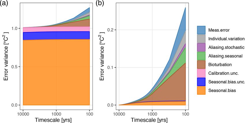
A. M. Dolman et al.: Timescale-dependent uncertainty – Part 2                                                                 829

2.4   The seasonal cycle                                            area in Fig. 3a but this time for the discrete spectrum of the
                                                                    deterministic sine wave seasonal cycle. In this situation, the
The often large cyclical variation in climate variables asso-       sign of the seasonal bias is unknown. It appears in the error
ciated with the seasonal cycle can also add noise to a proxy        spectrum as power at frequency zero.
record if the seasonal cycle is not adequately sampled by in-          If the timing of the production phase of the signal carri-
dividual signal carriers, each of which records a short por-        ers is known precisely, 1φc = 0, then the white noise vari-
tion of the cycle (Laepple and Huybers, 2013; Schiffelbein          ance is equal to the variance of the piece of the sine wave
and Hills, 1984). Additionally, a bias can be introduced in         that describes the portion of the year in which the carriers
the record if the signal carriers are produced in greater num-      are produced. In this case, the sign and value of the bias are
bers during a particular part of the year (Jonkers and Kučera,     completely “known” given the parameters of the model, or,
2015; Leduc et al., 2010). In the case of the orbital modula-       put another way, the proxy record can be attributed to the
tion of the amplitude of the seasonal cycle, this bias becomes      correct season.
a slowly varying error, and the variance of the noise process          PSEM can handle intermediate situations when, for exam-
also varies over the course of an orbital cycle (see Sect. 3.2      ple, we can parametrize with a proxy season length, τp , an
of Part 1).                                                         expected phase, hφc i, which is the midpoint of the proxy pro-
    In the spectral error model, the seasonal cycle is repre-       duction season, and an uncertainty in this phase, 0 < 1φc <
sented by the discrete power spectrum of a deterministic sine       2π. In this situation, there is both a bias with an expected
wave (Eq. 1 in Part 1). The interaction between this signal         value and sign and an uncertainty around this expected value
and seasonality in the production of signal recorders deter-        that comes from the phase uncertainty.
mines the magnitude of two errors: a white noise error gen-            Finally, if we include the amplitude modulation of the sea-
erated by the under-sampling of the seasonal cycle and a bias       sonal cycle over the course of a precessional cycle, σa2 > 0,
due to only sampling a portion of the seasonal cycle.               the size of any seasonal bias and bias uncertainty will vary
    We represent seasonality in the production of signal carri-     over time. In the spectral domain, this manifests as leakage
ers here by saying that production occurs continuously over         of power from frequencies lower than 1/T to higher frequen-
a set fraction of the year, τp (see Sect. 2.2 in Part 1). This      cies and creates additional timescale-dependent errors corre-
can also be viewed as a kind of filter, this time on the dis-       sponding to uncertain changes in the magnitude of seasonal
crete spectrum of the deterministic sine wave seasonal cycle.       biases between time periods. Additionally, the magnitude of
The transfer function of this filter can be constructed in an       aliased seasonal cycle variation will vary over a precessional
analogous way to those for bioturbation and slice thickness,        period (see Sect. 3.2 of Part 1).
and the difference between the filtered and unfiltered spec-
tra gives the error due to sampling only part of the seasonal       2.5   Measurement error and individual variation
cycle (see Sect. 3.2 in Part 1). Again, the finite time period
each carrier records means that the portion of the seasonal cy-     As a first order, the measurement error can be assumed to
cle during which signal carriers are created is sampled by the      be independent between measurements, and we simply add
individuals, and this generates additional redistributed white      the power spectrum of a white noise error term σmeas . More
noise in the proxy signal.                                          complex measurement errors such as machine drift or mem-
    In the absence of orbital modulation, four parameters de-       ory between measurements could be integrated by adding a
termine the errors generated by filtering and sampling the          power spectrum characterizing these machine characteristics.
seasonal cycle: σc2 , the variance of the full seasonal cycle;      We add an additional error term, σind , to account for inter-
τp , the proportion of the seasonal cycle during which signal       individual variation in the encoded signal. This is a catch-all
carriers are produced; hφc i, the expected midpoint (phase) of      term to include things like differences in depth habitat oc-
the signal carrier production; and 1φc , which represents un-       cupied by individuals and variation in the encoding of the
certainty in the phase of the carrier production (Sect. 2.5 in      signal, i.e., “vital effects” (Haarmann et al., 2011; Schiffel-
Part 1).                                                            bein and Hills, 1984; Sadekov et al., 2008; Duplessy et al.,
    If the signal carriers are produced all year round, τp = 1,     1970). For a given proxy measurement, the variance of this
there is no bias, and the white noise component has a vari-         term is scaled by the number of individual signal carriers in
ance equal to the variance of the full seasonal cycle divided       the sample, N.
by the number of signal carriers per sample, N.
    If the signal carriers are produced for only part of the        2.6   Calibration error
year, τp < 1, but with completely unknown timing (we do
not know which months, 1φc = 2π ), then the expected vari-          Finally, we add uncertainty in the proxy’s calibration to tem-
ance of this white noise is equal to the difference between         perature as a constant error, applying to all values in a given
the variance of the full seasonal cycle and the variance of the     record for which we do not know the sign but do have some
seasonal cycle filtered with a running mean filter of width, τp .   idea of the magnitude, σcal . This could, for example, be the
In the spectral domain, this is analogous to the gray shaded        standard error of the intercept term in a linear calibration

https://doi.org/10.5194/cp-17-825-2021                                                           Clim. Past, 17, 825–841, 2021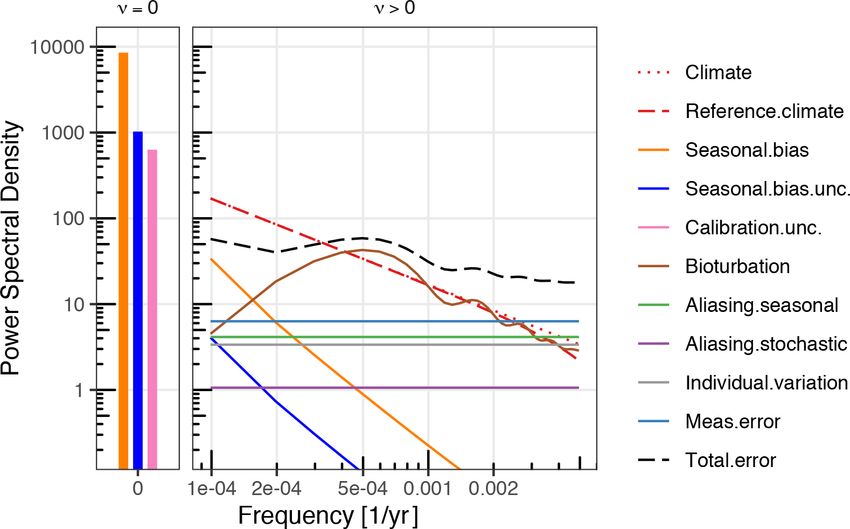
830                                                           A. M. Dolman et al.: Timescale-dependent uncertainty – Part 2

model. This is implemented as additional power at frequency          In contrast, the component due to bioturbation and sedi-
zero.                                                             ment slice thickness smoothing shows strong frequency de-
                                                                  pendence. The error due to smoothing is proportional to
                                                                  the variation in the climate signal; therefore, as variation in
2.7    Power spectrum of the total error                          the climate is larger at lower frequencies, the error due to
As the individual error components are independent, their         smoothing also increases towards lower frequencies. This is
power spectra can be added together to get the spectrum of        true up until the point at which the frequency examined ex-
the total error. Once the spectral error model has been pa-       ceeds the width of the smoothing filter, at which point the
rameterized for a given core, proxy, and sampling scheme,         error due to smoothing declines towards lower frequencies.
the resulting empirical power spectrum provides the magni-           The individual values in the record are most likely inter-
tude and full temporal correlation structure of the error com-    preted as a kind of mean of the time interval between ob-
ponents. From this, a number of useful quantities can be ob-      servations, and so we set the implicit reference timescale to
tained. These include the error in individual proxy measure-      be the same as the sampling resolution (1t = 100). For this
ments, the error after smoothing a record to a lower resolu-      example, the timescale of the bioturbation smoothing, τb , is
tion, the error in a time slice and in the difference between     1000 years. The large difference between these timescales
two time slices, and the expected correlation between repli-      implies a large error due to bioturbation smoothing. At fre-
cated proxy records. We illustrate these applications in the      quencies above about 2 times the bioturbation filter width,
following two sections.                                           the power of the bioturbation error is equal to the power of
                                                                  the reference climate.
                                                                     The timescale-dependent portions of the seasonal bias and
3     Illustration of the error spectrum approach for a           seasonal bias uncertainty are due to the orbital modulation
      hypothetical proxy record                                   of the amplitude of the seasonal cycle. As this is an ap-
                                                                  proximately 23 kyr cycle, these errors only become large at
We first illustrate the error spectrum approach for a hypothet-   timescales approaching 23 kyr.
ical 10 kyr foraminiferal Mg / Ca record. Parameter values
have been chosen to be realistic while ensuring that all com-     3.1   Timescale-dependent proxy error
ponents of the error model are presented. We parametrize the
climate spectrum as described in Sect. 2.1, assuming a sur-       The error for the individual proxy values at their original
face dwelling foraminifera at a virtual core position of 20◦ N,   sample resolution can be obtained by integrating the error
18◦ W calcifying between the surface down to 120 m (Fig. 2).      spectrum. When the record is smoothed before its interpreta-
We further assume that this taxon forms tests for a 7 month       tion, the timescale represented by each point changes, as does
period of the year, centered around the peak of the seasonal      the error. The error for a given timescale can be obtained
cycle but with an uncertainty in this phase of 2 months in ei-    by integrating the error spectra after first multiplying them
ther direction. A bioturbation depth of 10 cm and sedimenta-      by the transfer function of the smoothing filter (see Sect. 4,
tion rate of 10 cm kyr−1 are assumed. Thirty foraminifera are     Eq. 110 of Part 1).
picked from contiguous 1 cm thick sediment slices so that the        Timescale-dependent error for the example parameter set
resulting record has a sampling interval, 1t, of 100 years. We    is shown in Fig. 5 for timescales from 100 years (the original
assume a measurement error of 0.25 ◦ C and inter-individual       sampling resolution of the record) to 10 000 years (a mean
variation of 1 ◦ C. All parameters are given in Table 1.          or time slice of the entire length of the record), assuming a
   The power spectra of the individual error components, to-      running mean smoothing filter. The errors are shown on the
gether with their sum and the assumed power spectrum of the       variance scale so that they are additive and can be plotted
climate, are shown for this example parameter set in Fig. 4.      stacked together. The error(s) associated with the individual
Power at ν = 0 corresponds to errors that are constant for a      proxy measurements corresponds to the rightmost edge of
given proxy time series and thus do not shrink as additional      each subplot.
measurements are averaged together. Here it is composed of           Figure 5a includes error components that are constant for
those parts of the seasonal bias and bias uncertainty that are    a given record and do not shrink as a record is smoothed. For
constant over time (i.e., not orbitally modulated) and the cal-   example, a seasonal bias in a record due to signal carriers
ibration uncertainty.                                             (e.g., Foraminifera) preferentially recording a particular part
   The power spectral densities of the measurement error          of the seasonal cycle will not disappear as additional proxy
and individual variation components are horizontal lines,         measurements are averaged together. For this example here,
indicating that their power is independent of frequency,          the total error is dominated by the constant part of the sea-
i.e., that these error components have the property of            sonal bias component and to a lesser extent the bias uncer-
white noise. This applies also to the two components of           tainty and calibration uncertainty.
aliased/redistributed seasonal cycle and stochastic climate          Figure 5b includes only those error components that are
variation.                                                        at least partly independent between time points and there-

Clim. Past, 17, 825–841, 2021                                                         https://doi.org/10.5194/cp-17-825-2021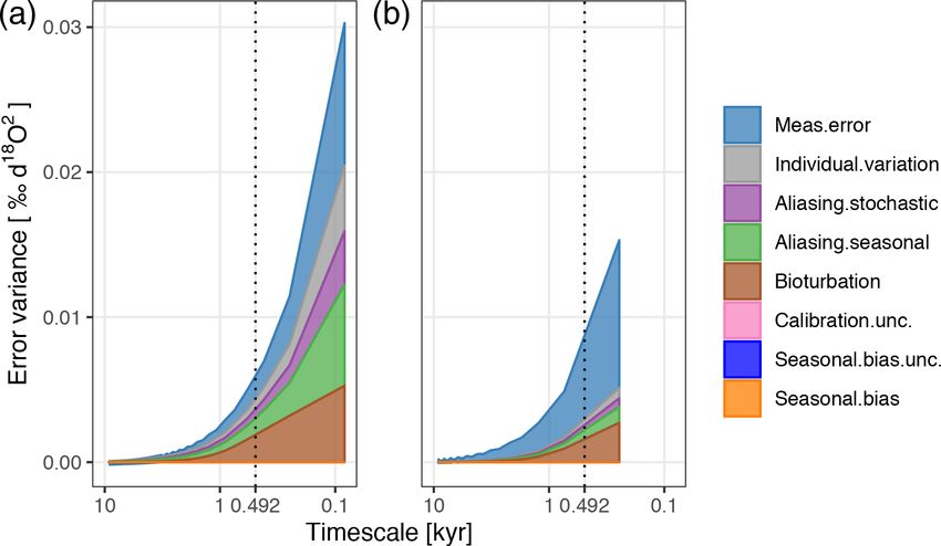
A. M. Dolman et al.: Timescale-dependent uncertainty – Part 2                                                                             831

Table 1. Parameters required for the spectral error model with their values in example 1 plus possible sources.

   Parameter     Value    Description                                                  Source
   1t              100    The sampling frequency of the proxy record (years)           Approximated by the mean sampling frequency of
                                                                                       an irregular time series
   τr              100    Interpreted timescale of the proxy time series (years)       Equal to 1t unless explicitly estimated
   T            10100     Total length of the proxy record (years)                     Odd multiple of 1t closest to the length of proxy
                                                                                       record
   τb             1000    Age heterogeneity of signal carriers due to bioturbation     The bioturbation depth (estimated) divided by the
                          (years)                                                      sedimentation rate or the age heterogeneity esti-
                                                                                       mated from replicated radiocarbon dates
   τs              100    Thickness of a sediment slice from which signal carriers     Sediment slice thickness divided by the sedimenta-
                          are extracted (years)                                        tion rate
   τp             7/12    Proportion of the year during which signal carriers are      Sedimentation trap data or predictions from a plank-
                          created                                                      tonic foraminifera model such as PLAFOM 2.0,
                                                                                       FORAMCLIM, or FAME
   hφc i             0    Expected phase of the signal carrier production period       Sediment-trap data or predictions from a plank-
                          relative to the seasonal cycle (−π, π )                      tonic foraminifera model such as PLAFOM 2.0,
                                                                                       FORAMCLIM, or FAME
   1φc           2π/3     Uncertainty in the phase of the signal carrier production
                          (0, 2π)
   N                30    Number of signal carriers per proxy measurement              Number of signal carriers per proxy measurement
   σc2              2.2   Variance of the seasonal cycle (proxy units2 )               Calculated from the modern climatological ampli-
                                                                                       tude of the seasonal cycle estimated from instru-
                                                                                       mental data, e.g., HadSST or reanalysis data
   σa2           0.014    Variance of the orbital modulation of the seasonal cycle     Inferred from orbital variation in incoming solar ra-
                          amplitude                                                    diation
   φa              π/2    Phase of the proxy record in relation to the orbital solar   Frequency of orbital cycle being modeled, e.g., pro-
                          radiation cycle                                              cession of 1/23 kyr
   σmeas           1/4    Measurement error (proxy units)                              Reproducibility of measurements on real world ma-
                                                                                       terial
   σind              1    Inter-individual variation (proxy units)                     Individual foraminifera studies
   σcal            1/4    Calibration error (proxy units)                              Standard error of the intercept term of a calibration
                                                                                       regression model

fore vary with timescale; i.e., it excludes errors that originate          when comparing proxy values from two time slices that are
from power at frequency zero. The component measurement                    far enough apart in time that any seasonal bias may differ
error, individual variation, and the aliased components of the             between the two time periods.
stochastic climate and seasonal cycle all decline rapidly with
timescale (i.e., as a record is smoothed with a running mean
to lower resolutions) as the errors are independent between                3.2   Error in a time-slice mean and the difference
samples and so decline inversely with the number of sam-                         between two time slices
ples being averaged together. The bioturbation component
declines more slowly as errors are positively autocorrelated               The information contained in the power spectra also allows
up until timescales of approximately 2τb . A portion of each               us to estimate the uncertainty in the difference in the climate
of the seasonal bias and bias uncertainty components does                  between two time points or between two time slices. A time
vary with timescale due to the orbital modulation of the am-               slice refers to an average taken over a set of proxy values
plitude of the seasonal cycle. They may become important                   within a certain time period of interest. For example, using
                                                                           the parametrization from Table 1, if we wanted to compare

https://doi.org/10.5194/cp-17-825-2021                                                                     Clim. Past, 17, 825–841, 2021
832 A. M. Dolman et al.: Timescale-dependent uncertainty – Part 2
Figure 4. Power spectra of error components of a climate proxy record. As the proxy record was sampled at 100-year resolution, only the
power-law portion of the climate power spectrum is visible. The error spectra are plotted on log–log axes with a broken frequency axis so
that power at the zeroth frequency (ν = 0) can be shown.
Figure 5. Timescale-dependent proxy error for an example parameter set. (a) Timescale-dependent error variance for all components of the
spectral error model. (b) Timescale-dependent error variance for all components excluding those that manifest as constant errors that do not
change with timescale, i.e., those originating as power at frequency zero.
the mean climate over the first and last 1000 years of the much smaller than the errors in the time slices themselves
proxy record, the error variance of each individual time slice (Fig. 6).
would be the value at timescale = 1000 years in Fig. 5. If all
the errors were independent in time, then the error variance
4 A working example: replicated Holocene δ18 O
of the difference between these two time slices would simply
records from southern Java
be the sum of the two variances. However, as some of these
error components are autocorrelated (or even constant over Here we illustrate the use of the error spectrum model on a
the entire time series), the covariance in the errors for the real proxy record by applying it to replicated foraminiferal
two time slices needs to be accounted for. The information to δ 18 O records taken from core GeoB 10054-4 off south-
do this is contained in the power spectrum of the error (see ern Java in the Indian Ocean collected during the R/V
Sect. 4; Eqs. 111–112 of Part 1). The uncertainty, or error, SONNE 184 expedition (8◦ 40.900 S, 112◦ 40.100 E; 1076 m
in the estimate of the difference between two time slices is water depth; Hebbeln and cruise participants, 2006). Repli-
Clim. Past, 17, 825–841, 2021 https://doi.org/10.5194/cp-17-825-2021A. M. Dolman et al.: Timescale-dependent uncertainty – Part 2 833
for the surface down to 50 m, resulting in an amplitude of
0.53 ‰.
At this location, G. ruber is thought to produce tests at an
approximately equal rate throughout the year and represent
the annual mean surface temperature in this region (Mohtadi
et al., 2011). We therefore set τp = 1, which implies year-
round production of signal carriers. As τp = 1, the parame-
ters hφc i and 1φc , which control the phase of signal carrier
production relative to the seasonal cycle, have no effect on
the error spectrum. Similarly, orbital modulation of the am-
plitude of the seasonal cycle will have only a small effect and
is ignored here.
The sediment accumulation rate estimated from the cal-
ibrated radiocarbon dates and retrieval depths is approxi-
mately 20 cm kyr−1 . The sediment slices were 1 cm thick, so
Figure 6. The uncertainty or error in the estimate of the mean cli-
τs was set to 50 years. A replicated set of radiocarbon dates
mate over two time slices covering the first and last 1000 years of
the pseudo-proxy record and the error in the estimate of the dif- taken from 10 samples each of 10 foraminifera indicated an
ference between these two time slices. The realistic error estimate inter-individual standard deviation in age of 720 years (un-
using PSEM (third column) is much smaller than the naive error published data) which we use for τb , corresponding to a bio-
estimate that one would obtain by just adding up the variances. turbation depth of about 14 cm.
For σmeas , we use the analytic replicability of 0.1 ‰, but
σind is more difficult to parametrize; we use 0.32 ‰, which
cated δ 18 O records were created using two different sampling was estimated by Sadekov et al. (2008) as the contribution of
schemes. In record 1 (Rep1), measurements were made on vital effects to replicability estimates for G. ruber.
samples consisting of five Globigerinoides ruber (s.s.) tests
each at a mean interval of 83 years; in Rep2, 30 tests of
G. ruber (s.s.) were used per sample at a mean interval of
246 years. An age model was constructed using nine AMS- 4.2 Timescale-dependent uncertainty
14 C dates on mono-specific samples of Trilobatus sacculifer
(see Supplement Table S1). The Marine13 radiocarbon cali- Total error variance at the highest frequency resolved (1t)
bration curve was used to calibrate the ages and construct a is much higher for Rep1 than Rep2 as there are fewer
linear age model (Reimer et al., 2013). As both records come foraminifera per sample so that the individual variation,
from the same core, more advanced age–depth modeling is aliased seasonal cycle, and aliased stochastic climate compo-
not required here. nents are all larger for Rep1 than for Rep2 (Fig. 7). The effect
A replicated set of radiocarbon dates taken from 10 sam- of this can be seen clearly in Fig. 8a which shows Rep1 and
ples each of 10 foraminifera indicated an inter-individual Rep2 at their original, irregularly sampled time points, to-
standard deviation in age of 720 years (Dolman et al., 2020), gether with their PSEM estimated uncertainties. Rep1 shows
which we use for τb , corresponding to a bioturbation depth much higher variance despite the fact that Rep1 and Rep2
of about 14 cm. come from the same sediment core and therefore both ex-
perienced the same climate signal and the same degree of
bioturbation smoothing.
4.1 Parametrization In Fig. 8b, Rep1 and Rep2 have both been interpolated
and smoothed to a regular 492-year resolution (492 = 2×1t
To assist potential users of PSEM, here we describe the pa- for Rep2). As the original time series were irregular, a dif-
rameter choices step by step. ferent number of proxy measurement now contribute to each
Formally, the spectral error model describes only regularly mean value. To account for this, we evaluate PSEM sepa-
sampled time series whose total length, T , is an odd multi- rately for each point, setting (1t) to the timescale, τsmooth ,
ple of the sampling interval, 1t. When applying the spectral divided by the number of original proxy measurements. Af-
error model to real proxy time series, we have to make some ter this smoothing, the two series are in much closer agree-
additional approximations to accommodate their inevitably ment. The error for Rep1 has shrunk much more than that
irregular (in time) sampling intervals. Hence, we approxi- for Rep2. In fact, smoothed to a timescale of 492 years, the
mate the sampling interval for each record, 1t, by 1t. error in Rep1 is now smaller than that in Rep2 due to the
For the climate spectrum, we again used a spliced empiri- larger number of proxy measurements contributing on aver-
cal and theoretical spectrum and estimated the amplitude of age to each point in the smoothed series (dotted vertical line
the seasonal cycle, as described in Sect. 2.1, but this time in Fig. 7).
https://doi.org/10.5194/cp-17-825-2021 Clim. Past, 17, 825–841, 2021834 A. M. Dolman et al.: Timescale-dependent uncertainty – Part 2 Figure 7. Timescale-dependent error variance for two different δ 18 O sampling strategies at GeoB 10054-4. (a) Five foraminifera per mea- sured sample with a mean time interval of 83 years between samples. (b) Thirty foraminifera per measured sample with a mean time interval of 246 years between samples. The vertical line at 0.492 kyr indicates the timescale to which the proxy records are smoothed in Fig. 8b. Figure 8. The δ 18 O records from GeoB 10054-4 (a) at their original temporal resolutions and (b) interpolated to a regular time series and smoothed to 492-year resolution. Shaded regions show 1σ error estimated using the PSEM. The error due to smoothing by bioturbation is excluded as it is deterministic and thus the same for each record. Numbers indicate the number of original data points contained in each averaged proxy value. Clim. Past, 17, 825–841, 2021 https://doi.org/10.5194/cp-17-825-2021
A. M. Dolman et al.: Timescale-dependent uncertainty – Part 2                                                                    835

Expected correlation with the true climate                           dividual measurements, these include the error after smooth-
                                                                     ing the record, the error in time slices, differences between
Finally, for the property of a proxy record, we are perhaps          time slices, and the expected correlation between replicates
most interested in is its correlation with the true climate. The     of a proxy record and between a record and the true climate.
proxy and climate can have low correlation due to a combi-           As with every model, some challenges remain, in particular
nation of non-climate variation (noise) in the proxy record          how to deal rigorously with the irregularity of real proxy time
and because variation in the climate has been smoothed out           series, the climate dependency of the habitat of the organisms
in the proxy record. As the noise and degree of smoothing            recording the climate signal, and the error associated with the
are timescale dependent, so too is the proxy–climate correla-        age uncertainty. Nevertheless, we argue that the spectral er-
tion. Using the power spectra of the errors and the assumed          ror approach represents a significant advance towards obtain-
power spectrum of the climate signal, we can calculate the           ing reliable uncertainty estimates for all quantities of interest
expected timescale-dependent correlation between the proxy           rather than single estimates applied uniformly to the record.
and climate. We do not in general know the true climate and             Although we have restricted the examples given here to the
so cannot test the accuracy of the climate–proxy correlation         Holocene, PSEM can be applied to other periods, albeit with
estimate; however, we can also calculate the expected corre-         greater uncertainty in its parametrization. Many of the er-
lation between replicate proxy records and use this as a par-        ror components, such as the bioturbation smoothing and sea-
tial test of the model under the assumption that only the pro-       sonal aliasing, should remain approximately correct; how-
cesses considered in PSEM affect the proxy record. The re-           ever, if we include glacial–interglacial cycles, there will be
sults (Fig. 9) indicate an increasing expected correlation from      larger variations in the sedimentation rate, and the seasonal-
around 0 at centennial timescales to around 0.5 at millennial        ity of the signal carriers (e.g., foraminifera) may change in
timescales. This is an upper bound estimate as the chrono-           unexpected ways. The amplitude of the seasonal temperature
logical uncertainty and other effects not considered here will       cycle and the precession-driven modulation of the seasonal
further decrease the climate-to-proxy relationship.                  cycle will vary with the longer inclination and eccentricity
   We estimated the timescale-dependent correlation be-              orbital cycles, although these changes are proportionally rel-
tween Rep1 and Rep2 using the R package corit (Reschke               atively small and deterministic. For the assumed stochastic
et al., 2019). The irregular time series were first interpolated     climate spectrum, the key issue is the assumption of station-
to high-resolution regular time series and then smoothed with        arity. If multiple glacial cycles are included, then one could
a set of increasingly wide running mean filters before calcu-        argue that the spectrum is again stationary and still domi-
lating the correlation between them. The observed correla-           nated by a power-law type variation. It becomes more dif-
tion between Rep1 and Rep2 is somewhat higher than that              ficult to justify if only one glacial–interglacial is included.
estimated from the error spectra (Fig. 9), perhaps indicating        Nonetheless, the PSEM approach should be a significant im-
that we have assumed, for example, a measurement error that          provement over assuming independent errors.
is slightly too high, although it is unclear if this difference is      Simulation-based forward modeling approaches such as
statistically significant. At timescales above 1000 years, esti-     sedproxy (Dolman and Laepple, 2018) and PRYSM (Dee
mates of the observed correlation become very variable due           et al., 2015) could also be used to estimate these quantities by
to there being very few effective data points left after smooth-     generating and summarizing over many simulated pseudo-
ing.                                                                 proxy records. The advantages of PSEM are that it provides
                                                                     an analytic understanding of the timescale dependence of er-
5   Discussion and conclusions                                       ror components while retaining the mechanistic understand-
                                                                     ing of the proxy generating process and can make these un-
Understanding the errors associated with climate proxies             certainty estimates rapidly for large sets of parameters, for
is an important task for paleoclimate research. Proxy er-            example, to directly model the error for a wide range of po-
rors, defined here as differences between the inferred cli-          tential sediment core characteristics (sedimentation rate and
mate and the unknown true climate, can be large and can              bioturbation depth) with different sampling schemes and at
thus strongly influence our understanding of past climate his-       different locations with differing climate properties such as
tory and the functioning of the climate system. Many compo-          seasonal cycle amplitude. This allows us to both better in-
nents of proxy error have a complex temporal autocorrelation         terpret the existing proxy record and to optimize future field
structure, making them timescale dependent and a challenge           work to answer specific questions.
to properly quantify and account for. The model introduced              Beyond modeling errors, PSEM also facilitates the use of
here (PSEM) and in the companion paper (Kunz et al., 2020)           the proxy variability itself to make inferences about the cli-
offers a rigorous and compact way to calculate and express           mate system. It allows us to predict the variability observed
this structure as error spectra, specifically here in this first     in individual foraminifera assemblages (IFAs) (e.g., Groen-
version for marine sediment cores. Once defined, the error           eveld et al., 2019; Thirumalai et al., 2019) and thus to directly
spectra can be used to calculate many quantities that will be        test the sensitivity of IFA statistics on the sedimentation rate,
useful to paleoclimate research. In addition to the error in in-     seasonality, or the spectrum of climate variability. Finally,

https://doi.org/10.5194/cp-17-825-2021                                                             Clim. Past, 17, 825–841, 2021
836 A. M. Dolman et al.: Timescale-dependent uncertainty – Part 2 Figure 9. Timescale-dependent correlation between replicated δ 18 O records at GeoB 10054-4 and their expected correlation with each other and with the true climate. The dark brown curve shows the observed timescale-dependent correlation between the replicate proxy records Rep1 and Rep2. The light brown and pink curves show the expected correlation between the two proxy records and between the proxy records and the true climate as calculated from the error spectra. The shaded areas indicate plus or minus the expected standard deviation in the correlation coefficients. PSEM provides the basis to develop spectral correction ap- Here, and in Part 1, we have defined analytical expressions proaches that infer the climate spectrum from the corrupted specifically for sediment-archived climate proxies; however, and distorted proxy spectrum, building on the approaches the approach is applicable to other proxy types as most proxy previously proposed for simpler sediment models (Laepple types experience similar error generation and distortion pro- and Huybers, 2013) or for aliasing only (Kirchner, 2005). cesses. For example, smoothing also affects water isotopes The PSEM version proposed here includes the sediment measured in ice cores via water vapor diffusion (Johnsen proxy processes described earlier for the proxy forward et al., 2000) and geochemical indices measured in coral model sedproxy (Dolman and Laepple, 2018) and represents records (Gagan et al., 2012) via successive incremental cal- a trade-off between complexity and completeness. For ex- cification in corals. These processes can also be expressed as ample, the interaction of seasonality in the recording and filters acting on the climate signal, and the power spectra of climate signal is the only slowly varying process so far in- the errors they produce are derived in a similar way. Thus, we cluded. However, the general formulation of the PSEM al- hope that PSEM presents an important step towards provid- lows other processes to be added. For example, depending ing more realistic error estimates for paleoclimate research. on the timescale of interest and the proxy type, other slowly varying processes, such as long-term changes in seawater Mg / Ca (Medina-Elizalde et al., 2008) or long-term instru- mental drift and memory effects of the measurement process, could be included by specifying the power spectra. When ac- counting for these processes, the use of PSEM vs. the clas- sical single-value uncertainty approach becomes even more important. Clim. Past, 17, 825–841, 2021 https://doi.org/10.5194/cp-17-825-2021
A. M. Dolman et al.: Timescale-dependent uncertainty – Part 2                               837

Appendix A: The influence of the assumed climate
spectrum on estimates of proxy error

An advantage of the spectral error method is that it does not
require a specific realization of a climate model; we do, how-
ever, need to make some assumptions about the statistical
properties of the true climate trajectory, which we encode via
an assumed power spectrum of the climate. Our approach is
to use a composite spectrum in which we splice an empirical
spectrum derived from observations for frequencies above
1/30 years with a theoretical power-law spectrum for lower
frequencies. In the examples presented in the main body of
the paper, we have assumed a slope of 1 for the power-law
portion of the spectrum. Here we test the sensitivity of the
method to the slope assumption by re-evaluating the error
spectra for the example in Sect. 3 using slopes of 0.5 and
1.5 in addition to 1 (Fig. A1). As changing the climate spec-
trum slope primarily influences the power at low frequencies,
the effect of this on proxy error depends on the scale of the
bioturbation; if bioturbation is so low that it integrates only
short-timescale climate fluctuations, then the influence of the
climate slope will be low. To illustrate this, we additionally
use values of 20, 200, and 2000 for the parameter τb , corre-
sponding to sedimentation rates of 5, 50, and 500 cm kyr−1
for sediment with a 10 cm bioturbation depth.
   Increasing the slope of the stochastic climate spectrum in-
creases the error components due to the smoothing of the
climate signal by bioturbation and the aliasing of this filtered
climate variation as a white noise error term (see Fig. A2).
However, the magnitude of these effects depends addition-
ally on the parameter τb controlling the timescale of the
smoothing filter. If τb is small, e.g., 20 years (Fig. A2a, b,
c), the increase in error is minimal as the change in climate
power only starts at frequencies below 1/30 years which are
barely influenced by the smoothing filter. The result of this
is that increasing the climate spectrum slope shifts the point
at which the power of the climate signal exceeds the total er-
ror spectrum to higher frequencies. For τb = 20 years, this
point shifts from approximately 1/1000 years with β = 1 to
1/333 years for β = 1.5. When β = 0.5, climate power re-
mains below the total error at all shown frequencies even
with very low bioturbation.
   For larger values of τb , the bioturbation filter smooths the
additional climate variation down to lower frequencies such
that the increase in bioturbation and aliasing error is larger,
offsetting the increase in climate power. For τb = 200, shift-
ing beta from 1 to 1.5 moves this from approximately 1/1000
to 1/500 years (Fig. A2d, e, f). For very large values of
τb corresponding to a sedimentation rate of 5 cm kyr−1 and
bioturbation depth of 10 cm (τb = 2000), increased climate
variation is almost completely offset by increased bioturba-
tion, smoothing error down to frequencies of 1/5000 years
(Fig. A2g, h, i).

https://doi.org/10.5194/cp-17-825-2021                             Clim. Past, 17, 825–841, 2021
838                                                               A. M. Dolman et al.: Timescale-dependent uncertainty – Part 2

Figure A1. Spliced empirical and power-law power spectrum of ocean temperature (0–120 m water depth) for 20◦ N latitude with slopes of
0.5, 1, and 1.5 for the low-frequency power-law region of the spectrum.

Clim. Past, 17, 825–841, 2021                                                             https://doi.org/10.5194/cp-17-825-2021
A. M. Dolman et al.: Timescale-dependent uncertainty – Part 2                                                                           839

Figure A2. A comparison of error spectra using different slopes for the power-law portion of the stochastic climate spectrum. Comparisons
are made for slopes, β, of 0.5, 1, and 1.5 and for different amounts of bioturbation smoothing with values for τb of 20, 200, and 2000 years.

https://doi.org/10.5194/cp-17-825-2021                                                                   Clim. Past, 17, 825–841, 2021
840                                                               A. M. Dolman et al.: Timescale-dependent uncertainty – Part 2

Code and data availability. The Proxy Spectral Error Model            References
(PSEM) is implemented as an R package. Its source code
is available from the public Git repository https://github.com/
EarthSystemDiagnostics/psem (last access: 24 March 2021). A           Bemis, B. E., Spero, H. J., Bijma, J., and Lea, D. W.:
snapshot of the R package at the time these analyses were performed      Reevaluation of the Oxygen Isotopic Composition of Plank-
is archived at Zenodo (https://doi.org/10.5281/zenodo.4271300,           tonic Foraminifera: Experimental Results and Revised Pa-
Dolman, 2020). Down-core radiocarbon dates and δ 18 O isotope            leotemperature Equations, Paleoceanography, 13, 150–160,
data for GeoB 10054-4 are provided in Supplement Table S1.               https://doi.org/10.1029/98PA00070, 1998.
                                                                      Berger, A. and Loutre, M.: Insolation Values for the Climate of
                                                                         the Last 10 Million Years, Quaternary Sci. Rev., 10, 297–317,
Supplement. The supplement related to this article is available          https://doi.org/10.1016/0277-3791(91)90033-Q, 1991.
online at: https://doi.org/10.5194/cp-17-825-2021-supplement.         Berger, W. H. and Heath, G. R.: Vertical Mixing in Pelagic Sedi-
                                                                         ments, J. Mar. Res., 26, 134–143, 1968.
                                                                      Bijma, J., Erez, J., and Hemleben, C.: Lunar and Semi-Lunar Re-
                                                                         productive Cycles in Some Spinose Planktonic Foraminifers, J.
Author contributions. TK, AMD, and TL designed the concep-
                                                                         Foramin. Res. 20, 117–127, 1990.
tual outline of the research. AMD coded the PSEM R package and
                                                                      Breitkreuz, C., Paul, A., Kurahashi-Nakamura, T., Losch,
produced the figures. AMD and TL wrote the paper with contribu-
                                                                         M., and Schulz, M.: A Dynamical Reconstruction of
tions from TK and JG.
                                                                         the Global Monthly Mean Oxygen Isotopic Composition
                                                                         of Seawater, J. Geophys. Res.-Oceans, 123, 7206–7219,
                                                                         https://doi.org/10.1029/2018JC014300, 2018.
Competing interests. The authors declare that they have no con-       Dee, S., Emile-Geay, J., Evans, M. N., Allam, A., Steig, E. J.,
flict of interest.                                                       and Thompson, D.: PRYSM: An Open-Source Framework
                                                                         for PRoxY System Modeling, with Applications to Oxygen-
                                                                         Isotope Systems, J. Adv. Model. Earth Sy., 7, 1220–1247,
Special issue statement. This article is part of the special issue       https://doi.org/10.1002/2015MS000447, 2015.
“Paleoclimate data synthesis and analysis of associated uncertainty   Dolman, A. M.: EarthSystemDiagnostics/Psem: Psem-Pub-Rev-
(BG/CP/ESSD inter-journal SI)”. It is not associated with a confer-      1, Zenodo, https://doi.org/10.5281/zenodo.4271300, 2020 (data
ence.                                                                    available at: https://github.com/EarthSystemDiagnostics/psem,
                                                                         last access: 24 March 2021).
                                                                      Dolman, A. M. and Laepple, T.: Sedproxy: a forward model for
Acknowledgements. This work was supported by the German                  sediment-archived climate proxies, Clim. Past, 14, 1851–1868,
Federal Ministry of Education and Research (BMBF) as a Research          https://doi.org/10.5194/cp-14-1851-2018, 2018.
for Sustainability initiative (FONA); through the PALMOD project      Dolman, A. M., Groeneveld, J., Mollenhauer, G., Ho, S. L., and
(FKZ: 01LP1509C). Thomas Laepple and Torben Kunz have re-                Laepple, T.: Estimating Bioturbation from Replicated Small-
ceived funding from the European Research Council (ERC) under            Sample Radiocarbon Ages., Earth Space Sci. Open Arch., pp.
the European Union’s Horizon 2020 research and innovation pro-           19, https://doi.org/10.1002/essoar.10504501.2, submitted, 2020.
gramme (grant agreement no. 716092). The work profited from dis-      Duplessy, J. C., Lalou, C., and Vinot, A. C.: Differen-
cussions at the CVAS working group of the Past Global Changes            tial Isotopic Fractionation in Benthic Foraminifera and
(PAGES) programme. We thank Henning Kuhnert for isotope analy-           Paleotemperatures Reassessed, Science, 168, 250–251,
ses, Mahyar Mohtadi for providing the sediment core GeoB 10054-          https://doi.org/10.1126/science.168.3928.250, 1970.
4, Nele Behrendt and Lena Kafemann for processing samples, and        Evans, M. N., Tolwinski-Ward, S. E., Thompson, D. M., and An-
Gesine Mollenhauer and Torben Gentz for radiocarbon dating.              chukaitis, K. J.: Applications of Proxy System Modeling in High
                                                                         Resolution Paleoclimatology, Quaternary Sci. Rev., 76, 16–28,
                                                                         https://doi.org/10.1016/j.quascirev.2013.05.024, 2013.
Financial support. This research has been supported by the Bun-       Fedorov, A. V., Brierley, C. M., Lawrence, K. T., Liu, Z.,
desministerium für Bildung und Forschung (grant no. 01LP1509C)           Dekens, P. S., and Ravelo, A. C.: Patterns and Mech-
and the European Research Council (SPACE; grant no. 716092).             anisms of Early Pliocene Warmth, Nature, 496, 43–49,
                                                                         https://doi.org/10.1038/nature12003, 2013.
The article processing charges for this open-access                   Gagan, M. K., Dunbar, G. B., and Suzuki, A.: The Effect of
publication were covered by a Research                                   Skeletal Mass Accumulation in Porites on Coral Sr / Ca and
Centre of the Helmholtz Association.                                     δ 18 O Paleothermometry, Paleoceanogr. Paleoclim. 27, PA1203,
                                                                         https://doi.org/10.1029/2011PA002215, 2012.
                                                                      Goosse, H., Renssen, H., Timmermann, A., Bradley, R. S., and
Review statement. This paper was edited by Denis-Didier                  Mann, M. E.: Using Paleoclimate Proxy-Data to Select Op-
Rousseau and reviewed by two anonymous referees.                         timal Realisations in an Ensemble of Simulations of the
                                                                         Climate of the Past Millennium, Clim. Dyn., 27, 165–184,
                                                                         https://doi.org/10.1007/s00382-006-0128-6, 2006.
                                                                      Groeneveld, J., Ho, S. L., Mackensen, A., Mohtadi, M., and Laep-
                                                                         ple, T.: Deciphering the Variability in Mg/Ca and Stable Oxygen

Clim. Past, 17, 825–841, 2021                                                              https://doi.org/10.5194/cp-17-825-2021
You can also read