Calibrating the soil organic carbon model Yasso20 with multiple datasets - GMD
←
→
Page content transcription
If your browser does not render page correctly, please read the page content below
Geosci. Model Dev., 15, 1735–1752, 2022
https://doi.org/10.5194/gmd-15-1735-2022
© Author(s) 2022. This work is distributed under
the Creative Commons Attribution 4.0 License.

Calibrating the soil organic carbon model Yasso20
with multiple datasets
Toni Viskari1 , Janne Pusa1 , Istem Fer1 , Anna Repo2 , Julius Vira1 , and Jari Liski1
1 Finnish   Meteorological Institute, Helsinki, 00101, Finland
2 Natural   Resource Center Finland, Helsinki, 00791, Finland

Correspondence: Toni Viskari (toni.viskari@fmi.fi)

Received: 4 August 2021 – Discussion started: 24 September 2021
Revised: 28 January 2022 – Accepted: 1 February 2022 – Published: 2 March 2022

Abstract. Soil organic carbon (SOC) models are important              et al., 2018; Thum et al., 2019) to quantify the global SOC
tools for assessing global SOC distributions and how carbon           stocks and estimate the effects of different drivers, such as
stocks are affected by climate change. Their performances,            changing environmental conditions, on SOC stocks (Sulman
however, are affected by data and methods used to calibrate           et al., 2018; Wiesmeier et al., 2019).
them. Here we study how a new version of the Yasso SOC                   While the majority of SOC models rely on linear equations
model, here named Yasso20, performs if calibrated individ-            representing the movement of C within the soil, there have
ually or with multiple datasets and how the chosen calibra-           been studies showing the need to represent at least some of
tion method affects the parameter estimation. We also com-            the SOC processes such as the microbial influence by non-
pare Yasso20 to the previous version of the Yasso model. We           linear equations (Zaehle et al., 2014; Liang et al., 2017) or
found that when calibrated with multiple datasets, the model          that the state structure of the model affects what kind of
showed a better global performance compared to a single-              data can be used to calibrate it (Tang and Riley, 2020). More
dataset calibration. Furthermore, our results show that more          complicated SOC models addressing these arguments have
advanced calibration algorithms should be used for SOC                been developed, for example Millennial (Abramoff et al.,
models due to multiple local maxima in the likelihood space.          2018), and modules including additional drivers affecting the
The comparison showed that the resulting model performed              C pools have been included in existing SOC models, such as
better with the validation data than the previous version of          nitrogen (Zaehle and Friend, 2010) and phosphorus (Davies
Yasso.                                                                et al., 2016; Goll et al., 2017) cycles. Their implementation
                                                                      is hindered, though, by the fact that detailed data are needed
                                                                      to constrain the model parameterization, but individual mea-
                                                                      surement campaign datasets are often limited in size and
1   Introduction                                                      lacking in nuance of the SOC state (Wutzler and Reichstein,
                                                                      2007; Palosuo et al., 2012). Consequently, multiple datasets
Soils are the second-largest global carbon pool, and hence            representing different processes should be used to parame-
even small changes in this pool impact the global carbon cy-          terize the models in order to capture the multitude of SOC
cle (Peng et al., 2008). However, soil organic carbon (SOC)           dynamics, but combining observation datasets with varying
and associated changes are difficult and laborious to measure         spatial scales, measurement temporal densities, inherent as-
(Mäkipää et al., 2008). They can also vary drastically over           sumptions, and structural errors can cause issues with ade-
space due to differences in litterfall, site, and soil type as well   quately incorporating all the information (Oberpriller et al.,
as climate (Jandl et al., 2014; Mayer et al., 2020). Hence,           2021). The chosen calibration methodology is additionally
SOC models are important tools for estimating current global          affected by the same issues based on its approach of fitting
soil carbon stocks and their future development (Manzoni              the data.
and Porporato, 2009). Numerous SOC models have been de-
veloped in the past decades (Parton, 1996; Camino-Serrano

Published by Copernicus Publications on behalf of the European Geosciences Union.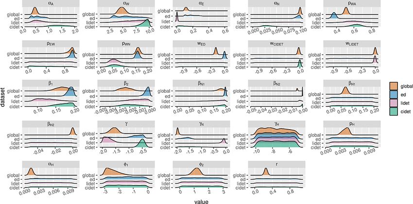
1736                             T. Viskari et al.: Calibrating the soil organic carbon model Yasso20 with multiple datasets

    Litter-bag decomposition experiments (Harmon et al.,             wherein there could be multiple parameter sets that can po-
2009) provide information on the faster decomposition pro-           tentially produce a local fit into the data. Last, but not least,
cesses, but their applicability to longer-term assessments has       the previous Yasso07 calibration workflow was not easily re-
been questioned (Moore et al., 2017). Furthermore, even              peatable and reproducible to allow inclusion of new datasets
in current studies it is common to use only data from one            and algorithms.
litter-bag decomposition experiment campaign (for example               In this study, we built upon previous Yasso developments
Kyker-Snowman, 2020) due to the differences in experimen-            to present a model formulation that expanded on how the en-
tal setups and physical properties of the litter bags, making        vironmental drivers affect the decomposition. The data used
direct comparison of results difficult. Organic carbon content       to calibrate the model are the same for both versions with
can be measured from soil samples, but those measurements            the exception of the measurement data regarding long-term
provide a limited snapshot because of the large number of            carbon allocation. For Yasso07, a time series dataset from
measurements needed to detect changes and the slow dynam-            southern Finland was used, while for Yasso20, approximated
ics of SOC (Mayer et al., 2020). Additionally, the SOC in            steady-state SOC measurements from across the world were
these measurements cannot effectively be fractionated into           used to constrain the relevant parameters. Additionally, we
different state components used in the models. Hence, as-            use a more advanced model calibration method in associ-
sumptions need to be made on the amount of short-lived SOC           ation with a stricter protocol on what kind of data points
to approximate the amount of long-lived SOC. There are also          were used for calibration and an open-source R package for
other aspects of litter that are known to affect the decomposi-      data inclusion, repetition, and reproduction of calibration.
tion rate, e.g. the bigger the size of the woody litter the slower   The model and produced parameter set will be referred to
the decomposition is (Harmon et al., 2000), which requires           as Yasso20 hereinafter. Our redesigned calibration protocol
detailed and specific observations to inform models.                 leverages the BayesianTools R package (Hartig et al., 2019),
    The Yasso07 model (Tuomi et al., 2009) was developed to          an open-source general-purpose tool for Bayesian model cal-
address some of these challenges. In it, both the litter inputs      ibration. Using BayesianTools in our workflow, we not only
and the soil carbon are divided into chemically measurable           established a more reproducible and standardized application
fractions that decompose at their own rate, which are affected       of Yasso20 calibration, but also leveraged interfacing with
by environmental conditions, specifically ambient tempera-           multiple calibration algorithms and examined the role of the
ture and moisture. This direct link between the model state          calibration method.
and litter input allowed using different litter decomposition           Due to the nature of the available SOC-related datasets we
experiment data to constrain model parameters. One of the            hypothesize the following: (i) the SOC model performs better
core ideas in the development of Yasso07 is that the parame-         globally if multiple datasets are simultaneously used to con-
terization process itself is done simultaneously with multiple       strain it compared to a SOC model calibrated with an indi-
datasets reflecting different parts of the SOC decomposition         vidual dataset despite the numerous assumptions required for
process in a Bayesian calibration framework (Zobitz et al.,          combining the different information; (ii) the likelihood space
2011). As a part of this approach, a litter-bag-specific leach-      created by these multiple datasets is uneven with multiple
ing term was introduced in order to be able to use information       maxima to the degree that more advanced parameter meth-
from several litter-bag experiments at the same time (Tuomi          ods are necessary for the end result not to be dependent on
et al., 2011b).                                                      the starting point; and (iii) these changes in the model for-
    While the initial Yasso07 calibration addressed challenges       mulation and the calibration protocol will improve how the
regarding the variety of data required, it did not touch in de-      Yasso model projections perform compared to the previous
tail on the issues affecting the actual SOC model parameter-         model version.
ization process. First, Yasso07 did not calibrate all the pa-           The first hypothesis is tested by calibrating Yasso with in-
rameters simultaneously with all the data, but instead cali-         dividual datasets as well as the combined datasets with the
brated the parameters in segments for which the previously           resulting performances compared using numerous validation
calibrated parameters were set as constant when calibrating          datasets. All these calibrations are done for all the parameters
the next set of parameters (Tuomi et al., 2011a). While this         simultaneously. The second hypothesis is tested by compar-
makes the calibration process easier, it naturally also affects      ing the Yasso parameter values produced by parameter es-
the results and associated uncertainties. Second, there have         timation methods of varying complexity and how well they
been no standard methods established to evaluate how the             converge. Furthermore, the more extensive calibration pro-
inclusion of additional datasets impacts the general perfor-         cess has allowed constraining more details in the new Yasso
mance of SOC models. In other words, does using multiple             formulation, which is introduced here as well.
datasets improve the model estimates? Naturally, this applies
to Yasso07 as well. Third, there have been studies which in-
dicate that the choice of parameterization method does mat-
ter in ecosystem modelling (Lu et al., 2017). It is reasonable
to assume that this would also hold true for SOC systems

Geosci. Model Dev., 15, 1735–1752, 2022                                               https://doi.org/10.5194/gmd-15-1735-2022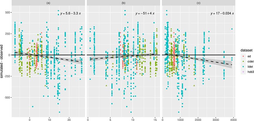
T. Viskari et al.: Calibrating the soil organic carbon model Yasso20 with multiple datasets 1737
2 Methods jority of them are from the surface. Thus, air temperature T
and precipitation P were used as the environmental drivers
2.1 Yasso model description along with the woody litter diameter d. Operator M is the
product of the decomposition, as presented by K, and mass
The Yasso model is based on four basic assumptions on lit- fluxes between compartments, as depicted by F :
ter decomposition and soil carbon cycle: (1) litter consists of
four groups of organic compounds (sugars, celluloses, wax- M (θ, c) = F (θ ) K (θ, c) , (2)
like compounds, and lignin-like compounds) that decompose
at their own rate independent of origin (Berg et al., 1982). −1 pWA pEA pNA 0
(2) Decomposition of any group results either in formation
pAW −1 pEW
pNW 0
of carbon dioxide (CO2 ) or another compound group (Oades, pAE pWE −1
F (θ ) = pNE 0 ,
(3)
1988). (3) The decomposition rate is affected by environment
pAN pWN pEN −1 0
temperature and moisture (Olson, 1963; Meentemeyer, 1978; pH pH pH pH −1
Liski et al., 2003). (4) The diameter size of woody litter de- K (θ, c) = diag. (4)
termines the decomposition rate (Swift, 1977). Yasso20 is
the next version of Yasso (Liski et al., 2005) and Yasso07 Here, parameters pij ∈ [0, 1] denote the flows from compart-
models (Tuomi et al., 2009, 2011b) and continues to build on ment i(i ∈ {A,W,E,N}) to j (j ∈ {A,W,E,N,H}) and are in-
these same assumptions. The main formulation contribution cluded in the parameter vector θ . The decomposition rates
in Yasso20 compared to the previous versions is the added ki (θ, c) were calculated according to
nuance in how climate drivers affect the different pools,
αi XJ 2
which in turn is possible here due to the improved calibra- ki (θ, c) = h (d) 1 − eγi P j =1
eβi1 Tj +βi2 Tj , (5)
tion scheme. For the purposes of the calibration here, another J
assumption was necessary: (5) the most stable soil carbon where the base decomposition rate αi , temperature parame-
compounds are only formed in the soil as a result of bond- ters βi1 and βi2 , and precipitation parameter γi for compart-
ing with mineral surfaces (Stevenson, 1982). The following ments i ∈ {A,W,E,N,H} are all a part of the parameter set θ .
model formulations apply for Yasso20. The temperature- and precipitation-dependent rate parame-
Based on the previously established assumptions, litter can ters are the same for compartments AWE, but both N and H
be divided into four fractions according to its chemical com- compartments are given their own separate parameter values.
position. Compounds soluble in a polar solvent (water) rep- In order to capture the annual temperature cycle more effi-
resent sugars (W), and those soluble in a non-polar solvent ciently, the average monthly temperatures for all 12 months
(ethanol or dichloromethane) represent wax-like compounds are given as an input with the model averaging over their im-
(E). Compounds hydrolysable in acid (for example, sulfu- pacts as seen in Eq. (5). The total annual precipitation is used
ric acid) represent celluloses (A), and the non-soluble and instead of monthly precipitation as seasonal variation such
non-hydrolysable residue represents lignin-like compounds as snowfall or heavy rainfall followed by long dry stretches
(N). Additionally, there is a fifth compartment, humus (H), would hinder the calibration if the monthly precipitation was
which represents long-lived, stable soil organic carbon pro- used. The temperature and precipitation equations are estab-
duced by interaction with mineral compounds in the soil. As lished in Tuomi et al. (2008). Woody litter decomposition
the carbon compounds are broken down by the decomposi- rate in response to diameter (d) is described in h(d) based on
tion processes, they become either new compounds belong- Tuomi et al. (2011a) as follows:
ing to another compartment or CO2 . The decomposition rate r
of each compartment is considered independent of the litter h (d) = min 1 + ϕ1 d + ϕ2 d 2 , 1 , (6)
origin and is affected by a temperature, moisture, and size
component.
where ϕ1 , ϕ2 , and r are parameters included in the parameter
The masses (x) of the compartments at time t are denoted
set θ.
by vector x(t) = [xA (t), xW (t), xE (t), xN (t), xH (t)]. The
Given initial state x0 , average environmental conditions c,
Yasso model uses an annual time step and determines the
and constant litter input b(t) = b, the model prediction can
changes in those masses according to
be computed by solving the differential equation in Eq. (1).
∂x (t) The solution becomes
= M (θ, c) x(t)T + b (t) , (1)
∂t
x (t) = M(θ, c)−1 eM(θ,c)t (M (θ, c) x0 + b) − b , (7)
where b(t) is the litter input to the soil at the time t, θ is
the set of parameters driving decomposition as defined in Ta- where the matrix exponential is determined numerically. In a
ble 1, and c contains the factors controlling the decomposi- steady-state situation x = limt→∞ x(t), Eq. (7) becomes
tion. Not only are accurate soil moisture estimates challeng-
ing to obtain for the measurements used here, but a vast ma- x = −M(θ, c)−1 b. (8)
https://doi.org/10.5194/gmd-15-1735-2022 Geosci. Model Dev., 15, 1735–1752, 2022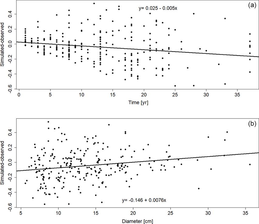
1738                               T. Viskari et al.: Calibrating the soil organic carbon model Yasso20 with multiple datasets

Table 1. The parameters, prior distributions, and initial values used in this calibration study. The initial values for the different chains were
randomly drawn from the prior distribution (U : uniform). If the starting value is listed as a set value, then the parameter was not varied in the
calibration and the given value was used for all chains.

       Parameter symbol    Parameter description                                              Prior distributions   Starting values
       αA                  Base decomposition rate for pool A (per year)                      U (0,2)               1.86, 0.23, 1.37
       αW                  Base decomposition rate for pool W (per year)                      U (0,10)              3.52, 6.0, 9.74
       αE                  Base decomposition rate for pool E (per year)                      U (0,2)               0.36, 1.63, 0.82
       αN                  Base decomposition rate for pool N (per year)                      U (0,0.1)             0.01, 0.06, 0.03
       αH                  Base decomposition rate for pool H (per year)                      U (0.001,0.01)        0.0024, 0.0094, 0.0045
       pAW                 Transference fraction from pool A to pool W                        U (0,1)               Set value of 1-pH
       pAE                 Transference fraction from pool A to pool E                        U (0,1)               Set value of 0
       pAN                 Transference fraction from pool A to pool N                        U (0,1)               Set value of 0
       pWA                 Transference fraction from pool W to pool A                        U (0,1)               0.31, 0.37, 0.68
       pWE                 Transference fraction from pool W to pool E                        U (0,1)               Set value of 0
       pWN                 Transference fraction from pool W to pool N                        U (0,1)               0.42, 0.45, 0.20
       pEA                 Transference fraction from pool E to pool A                        U (0,1)               Set value of 1-pEW -pH
       pEW                 Transference fraction from pool E to pool W                        U (0,1)               0.47, 0.91, 0.04
       pEN                 Transference fraction from pool E to pool N                        U (0,1)               Set value 0.
       pNA                 Transference fraction from pool N to pool A                        U (0,1)               Set value of 1-pH
       pNW                 Transference fraction from pool N to pool W                        U (0,1)               Set value of 0
       pNE                 Transference fraction from pool N to pool E                        U (0,1)               Set value of 0
       pH                  Transference fraction from AWEN pools to pool H                    U (0.001,0.01)        0.0071, 0.0064, 0.0026
       β1                  The first-order temperature parameter for AWE pools (per ◦ C)      U (0,0.2)             0.03, 0.04, 0.17
       β2                  The second-order temperature parameter for AWE pools (per ◦ C2 )   U (−0.05, 0)          −0.013, −0.007, −0.003
       βN1                 The first-order temperature parameter for N pool (per ◦ C)         U (0,0.2)             0.12, 0.01, 0.02
       βN2                 The second-order temperature parameter for N pool (per ◦ C2 )      U (−0.05, 0)          −0.24, −0.04, −0.03
       βH1                 The first-order temperature parameter for H pool (per ◦ C)         U (0,0.2)             0.002, 0.11, 0.20
       βH2                 The second-order temperature parameter for H pool (per ◦ C2 )      U (−0.05, 0)          −0.0001, −0.0014, −0.39
       0                   The precipitation impact parameter for AWE pools (year/mm)         U (−2, 0)             −0.93, −1.96, −1.34
       γN                  The precipitation impact parameter for N pool (year/mm)            U (−2, 0)             −1.66, −0.32, −0.63
       γH                  The precipitation impact parameter for H pool (year/mm)            U (−10, −5)           −9.65, −6.15, −5.47
       ϕ1                  The first-order impact parameter for size (per centimetre)         U (−3, 0)             −0.81, −1.41, −1.19
       ϕ2                  The second-order impact parameter for size (per cm2 )              U (3,0)               0.82, 0.25, 2.25
       r                   The exponent parameter for size                                    U (0,1)               0.83, 0.17, 0.49
       wED                 The leaching parameter for ED dataset                              U (−1, 0)             −0.08, −0.02, −0.05
       wCIDET              The leaching parameter for CIDET dataset                           U (−1, 0)             −0.03, −0.1, −0.08
       wLIDET              The leaching parameter for LIDET dataset                           U (−1, 0)             −0.08, −0.04, −0.02

Yasso20 improvements                                                        ibration results themselves, especially as this allows the en-
                                                                            vironmental conditions to impact the pools differently. Thus,
Two main changes were introduced to the Yasso20 ver-                        this changed model version was determined to be a new ver-
sion here compared to the earlier Yasso07 version. The first                sion of the model. We do not compare Yasso20 performance
change was that the temperature input for Yasso20 is given                  to Yasso07 here. All model parameters given in Table 1 were
as the mean monthly temperature for each month of the year                  targeted in the calibration.
instead of the mean annual temperature and associated an-
nual temperature amplitude. This was done in order to better                2.2    Datasets used in the calibration
represent the more nuanced global temperature profiles. For
example, the previous scheme was indifferent to whether the                 Several datasets were simultaneously used to calibrate the
winter was long or short, which is expected to affect the                   model in order represent different processes related to soil
annual decomposition. The second change was to differen-                    carbon cycling: decomposition bag time series data from the
tiate the climate driver impacts between the AWE, N, and                    Canadian Intersite Decomposition Experiment (CIDET; Tro-
H pools instead of using the same parameter values for all                  fymov and the CIDET Working Group, 1998), the Long-
the model C pools. This was done because previous research                  Term Intersite Decomposition Experiment (LIDET; Gholz et
established that more complex carbon compounds require                      al., 2000) and European Intersite Decomposition Experiment
more energy to be broken up (Davidson and Janssens, 2006),                  (ED; Berg et al., 1991a, b) projects, a collection of global soil
which indicates that the parameters representing those dy-                  organic carbon measurements gathered by Oak Ridge Na-
namics should also differ between pools. It is expected that                tional Laboratory (Zinke et al., 1986), and a woody matter
these changes will affect the model performance and the cal-                decomposition dataset from Mäkinen et al. (2006). In addi-

Geosci. Model Dev., 15, 1735–1752, 2022                                                        https://doi.org/10.5194/gmd-15-1735-2022
T. Viskari et al.: Calibrating the soil organic carbon model Yasso20 with multiple datasets                                  1739

tion to these large datasets, a smaller litter-bag decomposi-          The same litter-bag and woody data were used to cali-
tion dataset from Hobbie et al. (2005) was used to evaluate        brate both Yasso07 and Yasso20. The sole exception regard-
how much the addition of a comparatively small number of           ing the litter-bag data is that the whole ED dataset was used
data points affects the calibration results and an independent     in Yasso07 calibration, while in Yasso20 we removed de-
validation dataset for the other calibration parameters. These     composition data from manipulation experiments. However,
datasets along with additional details are listed in Table 2.      Yasso07 H pool parameters were not parameterized with the
    CIDET, LIDET, and ED are litter-bag decomposition time         Oak Ridge data. Instead, the chronosequence data from Liski
series with litter left to decompose in a mesh bag and the         et al. (1998) were used in its calibration with climate and
remaining mass measured at chosen time intervals over sev-         litterfall drivers derived from southern Finland conditions
eral years. Each dataset had the experiments with multiple         (Tuomi et al., 2009). As already established, this dataset was
different species, with the initial chemical composition also      not used in Yasso20 calibration and was only applied as a
provided by the dataset, and different sites. Furthermore,         validation dataset.
while CIDET and LIDET only measured the remaining mass,
ED also determines the AWEN fraction from one of the               Dataset uncertainties
replicant samples, which allows us to directly compare it to
the Yasso20 state variables. However, while in CIDET and           The information on the uncertainty related to the measure-
LIDET the remaining mass has ash removed, in ED ash is             ments was limited. With CIDET and LIDET there are gener-
still included in the remaining mass. The mean monthly tem-        ally four replicants, sometimes fewer, from which the stan-
peratures and precipitation have been measured at each test        dard deviation in remaining mass can be calculated. Similar
site with the annual precipitation being summed up from the        standard deviation is available for the ED measurements, but
monthly precipitation values.                                      it is only determined for the total mass loss and not for the
    The global SOC measurement dataset from Oak Ridge Na-          AWEN pool measurements used here. Furthermore, there are
tional Laboratory (Zinke et al., 1986) is a collection of data     other aspects affecting the uncertainties such as the ED mea-
from numerous unrelated projects that have measured SOC            surements containing ash or LIDET measurement time se-
as a part of their campaign. As such, there are no uniformly       ries showing more noise than the CIDET measurements. For
applicable protocols for these measurements. For the pur-          the global SOC dataset and the woody matter decomposi-
poses of the calibration, the data are assumed to represent        tion datasets no such replicant deviation is available nor is
the steady-state SOC at that location and each measurement         there any other established uncertainty. There are other sim-
is treated as independent from the others even if they are from    ilar measurement campaigns for which uncertainty estimates
the same location. Furthermore, we only used SOC measure-          are given, but it is not clear how directly they can be applied
ments that were below 20 kg C m−2 in the calibration. Values       for the datasets used here. Consequently, here we used our
higher than those were found in high latitudes and considered      expert opinion to determine the different dataset uncertain-
to be results of waterlogging, peat formation, or permafrost,      ties relative to each other (Table 1) as we felt this was a more
which are processes not described in Yasso20. The litter in-       transparent manner to acknowledge the current limitations
put was determined by combining the global gross primary           regarding assigning the uncertainties.
production (GPP) map from Beer et al. (2010) with the global           Systematic differences in the litter-bag properties affected
NPP–GPP (NPP: net primary production) relationship set to          the use of different datasets (Tuomi et al., 2009, 2011b). In
0.5 at the measurement locations due to lack of specific in-       general, high mass loss rates were positively correlated with
formation on the NPP–GPP there. The Olson classification           a large mesh size of the litter bags and high precipitation in
(Olson et al., 2001) regarding the local ecosystem type was        our datasets. This is because the decomposing material in the
used to roughly divide the ecosystems into grasslands, semi-       litter bags is partially “washed away” into the surrounding
forests, and forests. The litter fractioning for these different   soil by water flow and is thus removed from the bag due to
systems is given in Table S1. In addition, SOC chronose-           processes other than decomposing. To correct for this, we
quence data from Liski et al. (1998) and plot-level measure-       added a leaching term to Eq. (1) as follows:
ments of Liski and Westman (1995) were used as a validation        dx (t)
dataset.                                                                  = (A (θ, c) − ωsite P I5 ) x (t) + b (t) ,           (9)
                                                                    dt
    The woody decomposition data used here are from Mäki-
nen et al. (2006), which include measurements of multi-            where ωsite is the dataset-specific leaching term and I5 is a
ple trees in different stages of decomposition over several        5 × 5 identity matrix. This approach was simplified as there
decades in Finland. There are no signifiers to connect the         are multiple components expected to affect the leaching pro-
measurements from different years or to indicate how much          cess and other systematic errors, but it was necessary to es-
the tree diameter has been reduced over time because the data      tablish even this simplistic initial approach for the work here.
were not chronosequence data for the same trees. As such,              Finally, long-lived carbon compounds represented by the
the measurements were considered independent and repre-            H pool in the Yasso model are not produced in decomposition
sentative of decomposition of a tree trunk of that size.           litter bags as they require organo-mineral associations, which

https://doi.org/10.5194/gmd-15-1735-2022                                              Geosci. Model Dev., 15, 1735–1752, 2022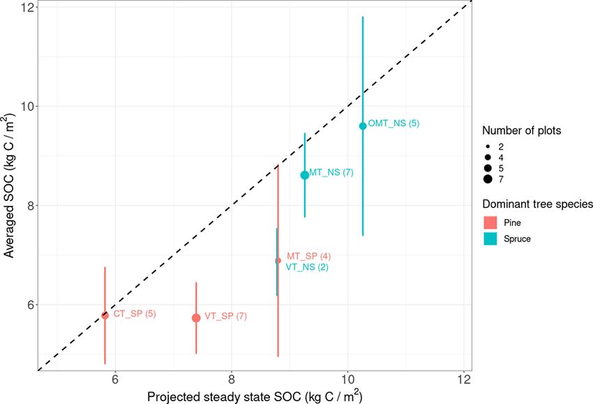
1740                                 T. Viskari et al.: Calibrating the soil organic carbon model Yasso20 with multiple datasets

Table 2. The measurement datasets used in this research.

  Data                    N     No. of   Time        T range      P range    Elevation   Uncertainty used    Note              Reference
                               species   range (a)   (◦ C)        (mm)       range (m)   in calibration
  Non-woody litter decomposition                                                                             Mesh size (cm)
  CIDET                1259        10    0–6         −9.8–9.3     261–1782   48–1530     100 g               0.25 × 0.5        Trofymow and the
                                                                                                                               CIDET Working Group
                                                                                                                               (1998)
  LIDET fine roots     2608         4    0–10        −7.4–26.3    150–3914   0–3650      200 g               0.055 × 0.055     Gholz et al. (2000)
  LIDET litter         5900        29    0–10        −7.4–26.3    150–3914   0–3650      200 g               0.055 × 0.056     Gholz et al. (2000)
  EURODECO             2184         5    0–5.5       0.2–7        469–1067   46–350      A: 40 g, W: 10 g,   1×1               Berg et al. (1991a, b)
                                                                                         E: 20 g, N: 40 g
  Hobbie                192         4    0–5         6.7          3676       270         100 g               0.3 × 0.2         Hobbie (2005)
  Woody litter decomposition                                                                                 Diameter (cm)
  Finland              1281         3    0–60        3.1          570        n/a         250 g               4.5–40.9          Mäkinen et al. (2006)
  SOC accumulation                                                                                           Soil depth (cm)
  Finland                26              5300        3            500        0           n/a                 0–30              Liski et al. (2005)
  SOC stock global     4113                          −26.9–28.0   0–5663     0–3900      7.5 kg              0–100             Zinke et al. (1986)
  Finland                30                          3.2          681        115–180     n/a                 0–100             Liski and Westman
                                                                                                                               (1995)
  Total               17 563

n/a: not applicable

are unlikely to occur in the litter layer and are only possible              uses adaptive subspace sampling to accelerate convergence
in the soil. Because of this pH (transfer fraction from AWEN                 (Vrugt, 2016). All three algorithms use proposal distribu-
pools to pool H) could have non-zero values only with the                    tions to generate successive candidate samples and grow the
Oak Ridge global SOC dataset.                                                chains. However, AM uses a multivariate Gaussian distribu-
                                                                             tion as the proposal, which is most effective when the target
2.3      Calibration protocol                                                distribution (also called the posterior) is also Gaussian. DEzs
                                                                             and DREAMzs algorithms use the differential evolution prin-
We used the BayesianTools R-Package (Hartig et al., 2019)                    ciple to optimize the multivariate proposals (with snooker
in our calibration workflow for its standardized and flexi-                  jumps to increase the diversity of the proposals) as well as
ble implementation of Markov chain Monte Carlo (MCMC)                        automatically adjust the scale and orientation of the proposal
algorithms with external models, as well as for its post-                    distribution according to the target distribution (Vrugt et al.,
MCMC diagnostic functionality. While our main aim in this                    2009; Vrugt, 2016). As a result of these properties, espe-
paper was not to compare MCMC algorithms, once the in-                       cially when not tuned properly, AM can take much longer
terface was established with the BayesianTools, it was trivial               to complete the high-dimensional parameter search and can
to leverage the common setup and test the performances of                    suffer from premature convergence when multiple distant lo-
different MCMC flavours as implemented by the package.                       cal optima are present (Vrugt, 2016; Lu et al., 2017). DEzs
We found this exercise helpful as our calibration problem in-                and DREAMzs can potentially resolve non-Gaussian, high-
volves a relatively high-dimensional and irregular likelihood                dimensional, and multimodal target distributions more effec-
surface. It has been previously shown that for such systems                  tively without much configuration (Laloy and Vrugt, 2012;
the efficacy of the calibration may differ between algorithms                Lu et al., 2017).
(Lu et al., 2017). Thus, we tested two robust and efficient al-                 In our calibration protocol, we ran three chains for each al-
gorithms: differential evolution Markov Chain with snooker                   gorithm through which DEzs and DREAMzs further tripled
updater (DEzs; ter Braak and Vrugt, 2008) and differential                   each chain. We initialized these chains from the prior distri-
evolution adaptive Metropolis algorithm with snooker up-                     butions (Table 1) using the random sample generator of the
dater (DREAMzs; Vrugt et al., 2009; Laloy and Vrugt, 2012;                   BayesianTools package. Each chain was run for 1.5 × 10⁶
Vrugt, 2016), in addition to the long-established adaptive                   iterations, and the last 1.5 × 10⁵ iterations were used to com-
Metropolis (AM) algorithm (Haario et al., 2001).                             pute the posterior probability distributions after removing the
   All three algorithms use Markov chains to explore the                     burn-in. Convergence diagnostics were checked by visually
parameter space and generate samples from the poste-                         inspecting the trace plots of the chains, as well as calculating
rior. However, AM uses a single chain, whereas DEzs                          the multivariate R statistic of Gelman and Rubin (1992).
and DREAMzs use multiple interacting chains simultane-
ously. While DREAM emerged from DE, DREAM further

Geosci. Model Dev., 15, 1735–1752, 2022                                                           https://doi.org/10.5194/gmd-15-1735-2022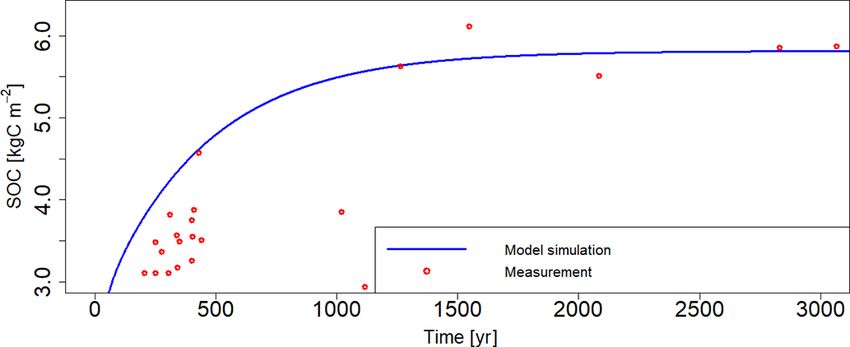
T. Viskari et al.: Calibrating the soil organic carbon model Yasso20 with multiple datasets                                  1741

   For the likelihood function we used a simple approach           calibration. In addition, the Hobbie3 dataset (Hobbie, 2005)
whereby the uncertainties are assumed to be normally dis-          was used as an independent validation dataset. Since there
tributed and independent of each other. In the litter-bag          was no information on its leaching parameter, that was set to
experiments, because the absolute uncertainty remains the          zero in the validation runs. The validation for each calibration
same over time while the amount of decomposing litter de-          was done with all the separate validation datasets. Similar
creases, the relative uncertainty increases over time. There       validation dataset is created with the Mäkinen wood decom-
are uncertainty dynamics affecting the data in reality that are    position data with 20 % of the data points set aside for val-
not accounted for here such as more nuanced time depen-            idation purposes. There was, however, no independent cali-
dence of the uncertainties, uncertainty auto-correlation in a      bration done with the Mäkinen dataset as there is not enough
time series, and non-normally distributed uncertainties. Due       data there to constrain the model completely, and in the vali-
to not having reliable information to properly assess how          dation analysis the focus was on how it performed over wood
these effects should be included into the likelihood calcu-        size instead of time.
lations here, we chose the described basic approach. This is          The global Oak Ridge SOC dataset was not split into cal-
considered to make it more straightforward to later add the        ibration and validation parts for two reasons. First, as it was
missing uncertainty dynamics as approximations of them be-         the only dataset calibrating the H parameters, there was no
come available and examine how those inclusions affect the         efficient to way to evaluate how the addition of new data
calibration results.                                               would have impacted the model performance regarding this
   Initially the calibration was done with all the parameters      dataset. Second, the dataset was found to be so noisy that
associated with the Yasso20 model. However, if the esti-           the randomized choosing of the validation data points al-
mated parameter values for the p terms in Eq. (3) were within      ready affected the results to a noticeable degree. Due to this,
three decimals from either 0 or 1, they were set to the near-      the H parameter calibration was evaluated with two separate
est limit value of 0 or 1, after which the calibration was re-     small datasets. First, SOC measurements from several plots
done. During the calibration, the p value parameterization         in Hyytiälä, Finland (Liski and Westman, 1995), where the
can never settle at 0 or 1, and hence it is impossible to know     dominant tree species of each plot is known, were used to
what the real p value is that close to the limit. The calibra-     test if Yasso20 was able to calculate an approximately cor-
tion results presented here only had four p values that were       rect SOC value for the plots. The SOC values for plots with
not set: pWA , pWN , pEW , and pEA . Parameters pAW and pNA        the same dominant species were averaged for the compar-
were set to 1 and the other AWEN-related p values were set         ison with the litterfall used for each species listed in the
to 0. Furthermore, since we assumed that only decomposi-           Supplement (Table S2). Second, an SOC chronosequence
tion in the W pool results in CO2 , we estimated only pEW          from Liski et al. (1998) was used to determine if Yasso20
and set pEA to be the E pool remnant from 1 with pEN set           is able to realistically simulate the SOC accumulation over
to 0.                                                              timescales of hundreds of years. In this dataset there are 26
                                                                   soil age gradient data points from the Finnish coast, which
2.4   Validation protocol                                          have been used to approximate the SOC accumulation in the
                                                                   soil over hundreds of years after the ice age. Tree litter and
Each of the litter decomposition experiments (CIDET,               climate driver data from Hyytiälä, Finland, were used here as
LIDET, and ED) was randomly split into two: data used for          the main focus is on whether the simulated system reaches
calibration (80 % of the measurements) and data used for val-      steady state in the same time window as the measurements.
idation (20 % of the measurements). Furthermore, the ran-          The climate driver data used for these validation runs are in-
dom division is done so that the whole measurement time            cluded in Table S3.
series from one bag is always fully either in calibration or
validation data. It was also verified that each site and species
                                                                   2.5   Yasso07–Yass020 comparison protocol
was approximately equally represented in both the calibra-
tion and the validation data. Due to the noise and bias in both
the global SOC measurement datasets in addition to the sep-        During the calibration of Yasso07, there was no separate val-
arate processes included in those calibrations, we did not di-     idation dataset aside from the CIDET, LIDET, and ED, and
vide them into calibration and validation parts but used all       all the data were used for the parameterization. Because of
the data for calibration.                                          that we do not use those validation datasets for the model
   The experiments were conducted by calibrating the Yasso         performance comparison. Instead, only the Hobbie3 valida-
model individually with the calibration data from each litter-     tion dataset and the Hyytiälä plots are used to determine if
bag decomposition dataset (CIDET only, LIDET only, ED              there is any notable improvement in Yasso20 performance
only) as well as a joint calibration that used all the calibra-    compared to Yasso07. For the litter-bag data, the comparison
tion data detailed before (i.e. CIDET, LIDET, ED, Mäkinen,         shall be the root mean square error (RMSE), while for the
global SOC). The leaching parameter was individually cal-          Hyytiälä plots the comparison is how the model-projected
ibrated for each decomposition bag dataset during the joint        steady-state SOC compares to the measured plot values.

https://doi.org/10.5194/gmd-15-1735-2022                                             Geosci. Model Dev., 15, 1735–1752, 2022
1742 T. Viskari et al.: Calibrating the soil organic carbon model Yasso20 with multiple datasets
To assess the differences in the model over long-term de- lowed by A, with N being the slowest to decompose. With
composition, both models were used to model the decom- the climate terms, both CIDET and LIDET calibrations have
position of a hypothetical straw litter (A = 620 g, W = 50 g, difficulties in settling on the climate terms while covering a
E = 20 g, N = 310 g) over a 100-year time period with the multitude of different climate types, while ED calibration,
Hyytiälä, Finland, climate drivers. This is not based on any whereby the climate differences between measurement loca-
measurement time series and is purely a synthetic test. tions are minor, produces a relative narrow climate parameter
estimate. The global calibration, however, does clearly con-
verge around certain climate parameters even if the uncer-
3 Results tainty range remains wide. And even though the ED dataset
has the most detail about the AWEN distribution, the AWE
3.1 Calibration performance
decomposition rates estimated based on it do not appear to
The first step was to determine if there is a notable differ- converge, with multiple peaks in the parameter distributions.
ence in how the different calibration methods perform with To further examine the parameter calibration, we analysed
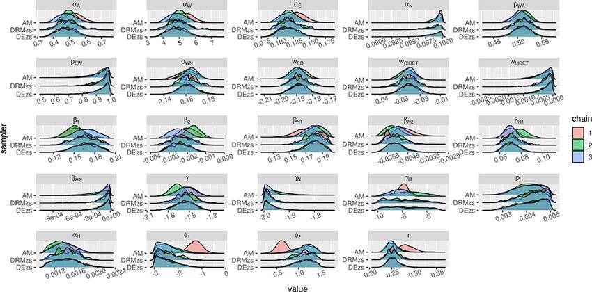
the global dataset. All three calibration methods (AM, DEzs, the correlations between different parameter values produced
DREAMzs) produced similar maximum a posteriori (MAP) by the DEzs algorithm from the global calibration (Fig. 3),
values for global (joint) calibration when all data streams which shows that the correlations are the strongest between
were used (Fig. 1, Table S4). Closer examination of differ- processes affecting the same pools. The p terms, which had
ent chains, though, shows that while DEzs and DREAMzs been set to 0 and 1, were excluded from the correlation anal-
converged to the same parameters, individual AM chains in- ysis since they did not vary during the calibration. The AWE
stead produced different parameter distributions, and thus the pool decomposition rates have strong positive correlations
calibration itself did not converge. The AM chain parame- between the decomposition rates and with the climate driver
ter distributions already settled into these distributions based terms affecting decomposition in them. Similarly, there is
on the initial parameter values given to them, and even after strong negative correlation between the temperature terms
doubling the number of iterations (not shown) the distribu- affecting the same pools and a strong positive correlation be-
tions remained the same. In our view, this is indicative of tween the H pool terms. There are both strong positive and
what would happen if a simple single-chain calibration was negative correlations with the size-related parameters. While
done with SOC models. The Gelman–Rubin (G–R) statistics the exact correlation values changed depending on the cal-
for the different calibration methods (Table S4) reflect these ibration dataset, the general relationships remained similar
differences in convergence as well, with DEzs having the val- (not shown).
ues within the acceptable boundary while values for AM are
above acceptable ranges. DREAMzs also performs generally 3.3 Validation and comparison to Yasso07
well but shows more divergence with the parameter values
than DEzs. Similar behaviour was seen when running the The final step was to validate how the different parameter
individual dataset calibrations; individual AM chains would sets perform with separate validation datasets and determine
mix well but converged at different values from each other if there are notable systematic errors with regard to the cli-
(not shown). Per global calibration diagnostics of different mate driver data. For each dataset, the RMSE values are at
algorithms, we decided to report the rest of the results with their lowest when using the parameter sets calibrated with
the DEzs algorithm for clarity as its estimates converged best that specific dataset (Table 3), though the global parame-
out of the three examined methods. When the global calibra- ter set produced RMSE values close to those lowest val-
tion with the DEzs algorithm was repeated with the Hobbie3 ues. However, when using the parameter sets calibrated by
dataset included, the resulting parameter distributions were datasets other than that one the validation data have been cho-
nearly identical to the calibration done without the Hobbie3 sen from, the RMSE values became higher, indicating worse
dataset included (not shown). model performance. When the RMSE analysis was done with
the Hobbie3 dataset, the global parameter showed the best
3.2 Parameter estimates and correlations performance. It should be noted that since in the ED dataset
measurements are for each individual AWEN pool, the indi-
The next step was to examine how the use of multiple vidual measurements are smaller in value than the total mass
datasets simultaneously affected the calibrated parameter measurements of CIDET, LIDET, and HOB3. Consequently,
sets compared to when using only individual datasets for cal- the RMSE values for ED are smaller than those for CIDET,
ibration. The parameter sets produced by the calibrations dif- LIDET, and HOB3 datasets.
fer from each other to a meaningful degree in both the param- With regard to the long-term SOC projections, the compar-
eter mean value and the associated uncertainty range (Fig. 2; isons with the Hyytiälä forest plot measurements (Table 4;
Table S5). Despite that, though, there are certain patterns in Fig. 4) indicate that at least in the Nordic forests Yasso20
the parameter sets: the pool decomposition rate relationships potentially slightly overestimates the steady-state SOC, with
remain the same in that W has the quickest turnover rate fol- the largest differences still being below 2 kg C m−2 . It should
Geosci. Model Dev., 15, 1735–1752, 2022 https://doi.org/10.5194/gmd-15-1735-2022T. Viskari et al.: Calibrating the soil organic carbon model Yasso20 with multiple datasets 1743 Figure 1. The global calibration results with the different calibration methods. Figure 2. The estimated parameter distributions using DEzs with different calibration datasets. be noted, though, that there is notable variance within the est plot measurements (Table 4), in all plots Yasso07 overes- measurements in addition to the uncertainty related to the timated the SOC by at least 3 kg C m−2 more than Yasso20. driver data. The chronosequence data (Fig. 5) show that the However, when examining the distribution of carbon into dif- model projection saturates in approximately 1000 years, sim- ferent pools in these steady states (not shown), more mean- ilarly to the measurements. ingful differences were revealed. For Yasso07, only ∼ 37 % When examining how Yasso20 performs relative to of the SOC was in the long-lived H pool, while ∼ 50 % of Yasso07, the RMSE for Yasso07 projections is 118.2 g com- the carbon was in the N pool. By comparison, with Yasso20 pared to the Yasso20 RMSE of 110 g. With the Hyytiälä for- https://doi.org/10.5194/gmd-15-1735-2022 Geosci. Model Dev., 15, 1735–1752, 2022
1744                              T. Viskari et al.: Calibrating the soil organic carbon model Yasso20 with multiple datasets

Table 3. The RMSE values for the different validation datasets when the model is run with the MAP values from the calibrations done with
the different datasets. As with the measurements, the RMSE unit here is grams. The lowest RMSE for a particular dataset is bolded.

                   Validation dataset    CIDET calibration     LIDET calibration    ED calibration    Global calibration
                   CIDET                               109.0               128.8             226.4                115.5
                   LIDET                               224.3               168.8             345.4                199.9
                   ED                                   49.5                55.0              35.5                 40.3
                   Hob3                                133.8               126.6             367.0                110.0

Table 4. Averaged measured SOC and projected SOC values with both Yasso07 and Yasso20 for forest plots in Hyytiälä, Finland, classified
by measurement site (units: kg C m−2 ).

                     Site ID (dominant tree species;    Averaged SOC           Yasso20 projected     Yasso07 projected
                     number of plots)                   (standard deviation)   steady-state SOC      steady-state SOC
                     CT_SP (pine; 5)                    5.78 (0.97)            5.82                  8.32
                     VT_SP (pine; 7)                    5.73 (0.71)            7.39                  10.61
                     VT_NS (spruce; 2)                  6.86 (0.67)            8.78                  13.06
                     MT_SP (pine; 4)                    6.89 (1.93)            8.80                  12.78
                     MT_NS (spruce; 7)                  8.61 (0.84)            9.26                  13.87
                     OMT_NS (spruce; 5)                 9.6 (2.2)              10.26                 15.47

                                                                         Figure 4. The projected steady-state SOC compared to the averaged
                                                                         measured SOC values in plots from multiple measurement sites.

Figure 3. Parameter correlations for the global calibration with the
DEzs algorithm.

projections ∼ 54 % of the carbon is in the long-lived H pool
and ∼ 27 % in the N pool.
   The hypothetical straw litter decomposition (Fig. 6) shows
that while the total carbon remainder amounts for the two
models are close to each other for the first 10 years, after that        Figure 5. Measurement-based (red dots) and model-based (blue
there is a clear divergence between the model projections,               line) projections of SOC accumulation on the Finnish coast after
with Yasso07 having more remaining carbon than Yasso20.                  the end of the ice age.
More detailed inspection of the results (not shown) found
that this difference was due to the N pool decomposing at a
much slower rate than in Yasso07 than in Yasso20. This also

Geosci. Model Dev., 15, 1735–1752, 2022                                                   https://doi.org/10.5194/gmd-15-1735-2022
T. Viskari et al.: Calibrating the soil organic carbon model Yasso20 with multiple datasets 1745
were lacking, confirming our first hypothesis. This is in line
with prior studies arguing for larger representation in the cal-
ibration data (Zhang et al., 2020). Furthermore, a more de-
tailed analysis of different calibrations shows (Fig. 2) that
the information from multiple datasets is in truth even nec-
essary for the calibration, as when calibrating only with
one dataset, the decomposition parameter uncertainty ranges
were either large or, in the case of the more nuanced EU-
RODECO dataset, did not even appear to converge. Some-
thing that was not examined in this study was how the un-
certainties for the different datasets should be defined. Even
if the assigned measurement uncertainties were correct for
each dataset, combining them introduces structural uncer-
tainties that should also be accounted for (MacBean et al.,
2016). A potential method to address this would be to esti-
mate the dataset uncertainties along with the model parame-
ters, as done, for example, in Cailleret et al. (2020), but ap-
plying this approach to the SOC system will require a more
Figure 6. The remaining decomposing carbon for a hypothetical thorough analysis in order to assess how it impacts the re-
straw litter in Hyytiälä, Finland, climate conditions when simulated sults.
with Yasso07 (solid red) and Yasso20 (dashed blue) with a (a) 20-
year and (b) 100-year time window. Further inclusion of smaller dataset
Even with this global calibration, individual locations can be
causes less carbon to accumulate in the H pool in Yasso07 affected by specific SOC decomposition conditions not cur-
than in Yasso20, with the latter having approximately twice rently accounted for in models (Malhotra et al., 2019). Natu-
as much carbon in the H pool than the former after 50 years. rally, if smaller datasets of SOC and decomposition measure-
When repeated with warmer climate drivers (not shown), the ments are available from locations affected by specific de-
Yasso07 time series projection decreases at a faster rate than composition dynamics, for example agricultural soils that are
the Yasso20 time series projection. treated in a very specific manner, it would be logical to use
that local information to constrain the SOC model to better
3.4 Residual analysis suit that location. However, the results here raise questions
on how those smaller datasets should be implemented in the
When checking residuals from the litter-bag experiments
model calibration. The inclusion of the Hobbie3 dataset did
against mean annual temperature, annual temperature vari-
not meaningfully impact the calibration results (not shown),
ation, and total annual precipitation (Fig. 7), there appears to
which is reasonable considering how small that litter-bag
be a tendency for Yasso20 to increasingly underestimate the
dataset (N = 192) is compared to the totality of the other
remaining litter-bag C with growing average mean tempera-
datasets (N =∼ 17 000 of which Nlitter bag =∼ 12 000) used
ture and precipitation. The error does not, though, show any
in the calibration. This indicates that due to the sheer size of
signal when looking at the temperature variation within the
the global calibration dataset, smaller local datasets cannot
year. With the woody decomposition residuals (Fig. 8), there
effectively be used just by adding them to the joint calibration
is a slight negative trend over time and a slight positive trend
process. Additionally, while the smaller datasets such as the
over size. Both are minor, though, and the residuals for the
Hobbie3 dataset contain site-specific information, they are
woody decomposition are relatively evenly distributed for the
measurements similar to the ones within CIDET and LIDET,
validation dataset.
and thus there is no reason to believe they would provide ad-
ditional insight into the global application. There are other
4 Discussion options, though, by either using the globally estimated pa-
rameter ranges as the priors for a calibration with the local
4.1 The benefit of calibrating with multiple datasets data, re-weighing the different datasets based on expert opin-
ion (Oberpriller et al., 2021), or employing a hierarchical cal-
Our results show that simultaneously using multiple datasets ibration approach (Tian et al., 2020; Fer et al., 2021), but the
from different environments improves the general applica- impact of these approaches should be separately researched
bility of the SOC model even when the simplistic leaching and tested. Our study still successfully provided a global pa-
factor approach had to be used to be able to compare dif- rameter set that increases the applicability of the Yasso model
ferent litter-bag datasets and detailed uncertainty estimates and informs global SOC estimates.
https://doi.org/10.5194/gmd-15-1735-2022 Geosci. Model Dev., 15, 1735–1752, 20221746 T. Viskari et al.: Calibrating the soil organic carbon model Yasso20 with multiple datasets
Figure 7. Residual analysis between simulated and observed carbon remnant on (a) mean temperature (◦ C), (b) temperature variation (◦ C),
and (c) total precipitation (mm yr−1 ) at the validation site.
to the local likelihood maxima and that the resulting param-
eter sets were strongly affected by the starting values. This
supports our second hypothesis that more advanced calibra-
tion methods are necessary to better explore the likelihood
surface and estimate SOC model parameters due to the trade-
offs between the parameter values that result in equifinality in
the parameter space. Furthermore, even the more stable cal-
ibration method produced different results for different indi-
vidual datasets used to calibrate. More advanced calibration
methods, though, then need to be applied to minimize the
impact of the resulting uneven parameter space and produce
Gelman–Rubin values within more acceptable ranges (Gel-
man and Rubin, 1992). Something that was curious in our
results was that DEzs converged better than DREAMzs (Ta-
ble S4) despite the latter being a more state-of-the-art method
(Vrugt, 2016). We were not able to specifically determine the
reason for this in our tests here; was it something related to
the behaviour of the parameter space or to some aspect of the
Figure 8. Residual analysis between simulated and observed carbon technical implementation?
remnants of wood decomposition from Mäkinen et al. (2006) on
(a) decomposition time and (b) diameter. 4.3 Impact of prior parameter information
One of the fundamental challenges for calibrating SOC mod-
4.2 Calibration method els is lack of experimental information regarding the model
parameter value distributions. Therefore, we used generally
Here we showed that by using a DEzs calibration algorithm, broad uniform prior distributions for the calibration here.
we were able to simultaneously use multiple different types However, it is still important to evaluate the calibration re-
of datasets to constrain the soil organic carbon (SOC) model sults based on our understanding of the overall system be-
Yasso and produce a converging parameter set. Additionally, haviour. For example, initially we used wider priors for pa-
using a more conventional model calibration approach, here rameters pH and αH (results not shown), which in turn re-
the adaptive Metropolis (AM), showed that it was vulnerable sulted in the calibration producing a pH value of ∼ 0.08
Geosci. Model Dev., 15, 1735–1752, 2022 https://doi.org/10.5194/gmd-15-1735-2022T. Viskari et al.: Calibrating the soil organic carbon model Yasso20 with multiple datasets 1747 and, consequently, a much higher H pool decomposition rate. from individual datasets (Fig. 2) there are parameter sets As this did not fit the system behaviour seen, i.e. with the there which have similarly low decomposition rates for the N bare fallow experiments (Menichetti et al., 2019) or the soil pool as Yasso07. Depending on how the different measure- chronosequence (Fig. 3), we applied a narrower prior con- ment datasets were weighed, it might be that those datasets straint on the related parameters. Another, and a more com- that favoured slower N pool decomposition had more im- plicated, example is that when using wider prior constraints pact than with Yasso20 calibration. Finally, in Yasso20 the for the N pool decomposition rate parameter αN , the cali- climate driver parameters are different between the AWE bration resulted in the N pool being largely insensitive to and N pools, and while the temperature terms are close to the temperature and moisture drivers. While there are no di- each other, the precipitation terms do differ from each other, rect measurements of the lignin pool temperature sensitivity, while in Yasso07 they would be the same. This would affect there have been studies showing that the energy needed for the Yasso07 dynamics during calibration. The calibration is breaking down SOC compounds increased with complexity made even more vulnerable to all these factors because a vast (Davidson and Janssens, 2006; Karhu et al., 2010), indicat- majority of the litter-bag data used here are from the first ing that the N pool should be temperature-sensitive. Here we 6 years of decomposition during which Yasso07 and Yasso20 chose to constrain αN to a lower range, which in turn forced a are very close to each with regard to total carbon remain- climate driver sensitivity for it. All these examples illustrate ing (Fig. 6). In such a situation it is very possible that less- that prior information and expert opinion should directly in- developed calibration protocols can lead to unrealistic sys- form the calibration, and the calibration results themselves tem dynamics that still appear to produce good results within should be further reassessed in their physical meaning. limited time windows. 4.4 How Yasso20 performs in comparison to Yasso07 4.5 Leaching When comparing the litter-bag validation dataset perfor- As established in Sect. 2.2, in order to compare the measure- mances of Yasso07 and Yasso20, there is an improvement ments from different litter-bag experiments, there needs to be with Yasso20 even though both models have been calibrated a parameter that accounts for the litter-bag type’s impact on largely with the same litter-bag data. This underlines the fact the mass loss rate (Tuomi et al., 2009). When testing with that the added model detail and reconsidered calibration pro- independent litter-bag data, we see that even with this added cess have a positive impact on the model projections. What assumption, the global calibration produces a better fit than is more striking, though, is that Yasso20 did perform better the calibration based on individual litter-bag campaigns (Ta- across the board with the Hyytiälä SOC data than Yasso07 ble 3). This supports using data from multiple litter-bag cam- when the latter model’s long-term SOC component was cali- paigns in model calibration. However, in the results it is ev- brated with Finnish conditions. This result argues that while ident that not only are the leaching parameters estimated to local calibration data are important, even for those specific be essentially zero when calibrating only with individual de- locations there could be a benefit in including global data composition bag datasets (Table S5), but also when simulta- in the calibration. These results validate the third hypothe- neously calibrating with all the datasets, only the ED dataset sis concerning the impact of the presented improvements on ends up having a meaningfully non-zero value. First of all, model performance. this indicates that the current straightforward formulation for A more thorough analysis of the model projections re- leaching is insufficient; as with the individual dataset cali- vealed a more fundamental difference in the model dynam- brations, the other parameter values are able to produce fits ics than initially indicated by the comparison datasets. In where there is no leaching despite knowledge that it is a fac- Yasso07 the N pool decomposes much slower, which impacts tor. Second, even when calibrating multiple datasets simulta- the rest of the decomposition dynamics and causes less long- neously, the calibration appears to apply the leaching effect lived H pool carbon to be formed during the soil decomposi- to only one of the datasets even when it should affect all of tion. As a consequence of differences in the calibration pro- them. cedures and the resulting model versions, Yasso07 projects A further complication is that the differences in RMSE re- higher SOC values than Yasso20 with the same input val- sults (Table 3) suggest that there are systematic differences ues, and these model versions would also react differently to between the datasets resulting from various sources such as changes in climate conditions and litter input. the experimental setup or environmental differences. As a The Yasso07 dynamics are most likely due to a combi- consequence, calibrating with these kinds of datasets will re- nation of multiple factors, which highlights the complicated sult in systematic differences in model performance as estab- process of SOC model calibration. As Yasso07 was cali- lished in Oberpriller et al. (2021) and as can be seen in how brated in segments, the woody decomposition parameters CIDET- and LIDET-calibrated Yasso performs with the ED were calibrated after the AWEN H pool parameters were de- dataset and vice versa. By being a corrective term, the leach- termined from the global litter-bag experiments and Finnish ing factor introduced here will also reflect all those other ele- SOC measurements. When looking at the calibration results ments causing the systematic differences, for example differ- https://doi.org/10.5194/gmd-15-1735-2022 Geosci. Model Dev., 15, 1735–1752, 2022
You can also read