Development and evaluation of 0.05 terrestrial water storage estimates using Community Atmosphere Biosphere Land Exchange (CABLE) land surface ...
←
→
Page content transcription
If your browser does not render page correctly, please read the page content below
Hydrol. Earth Syst. Sci., 25, 4185–4208, 2021
https://doi.org/10.5194/hess-25-4185-2021
© Author(s) 2021. This work is distributed under
the Creative Commons Attribution 4.0 License.

Development and evaluation of 0.05◦ terrestrial water
storage estimates using Community Atmosphere
Biosphere Land Exchange (CABLE) land surface
model and assimilation of GRACE data
Natthachet Tangdamrongsub1,2 , Michael F. Jasinski2 , and Peter J. Shellito3
1 Earth
      System Science Interdisciplinary Center, University of Maryland, College Park, Maryland, USA
2 Hydrological
             Sciences Laboratory, NASA Goddard Space Flight Center, Greenbelt, Maryland, USA
3 Oxbow Science, LLC, Seattle, WA, USA

Correspondence: Natthachet Tangdamrongsub (natthachet.tangdamrongsub@nasa.gov)

Received: 19 December 2020 – Discussion started: 14 January 2021
Revised: 5 June 2021 – Accepted: 7 June 2021 – Published: 29 July 2021

Abstract. Accurate estimation of terrestrial water stor-        proved model parameters and improved state estimations (via
age (TWS) at a high spatiotemporal resolution is important      GRACE DA) together is recommended to achieve the best
for reliable assessments of regional water resources and cli-   GWS accuracy. The workflow elaborated on in this paper re-
mate variability. Individual components of TWS include soil     lies only on publicly accessible global data sets, allowing the
moisture, snow, groundwater, and canopy storage and can be      reproduction of the 0.05◦ TWS estimates in any study region.
estimated from the Community Atmosphere Biosphere Land
Exchange (CABLE) land surface model. The spatial reso-
lution of CABLE is currently limited to 0.5◦ by the reso-
lution of soil and vegetation data sets that underlie model     1   Introduction
parameterizations, posing a challenge to using CABLE for
hydrological applications at a local scale. This study aims     Accurate knowledge of terrestrial water storage (TWS) is
to improve the spatial detail (from 0.5 to 0.05◦ ) and time     crucial for assessing water resource and climate variability
span (1981–2012) of CABLE TWS estimates using rederived         (Delworth and Manabe, 1988; Koster and Suarez, 2001).
model parameters and high-resolution meteorological forc-       TWS consists of soil moisture, groundwater, snow, and
ing. In addition, TWS observations derived from the Gravity     canopy storage. Each component plays a significant role in
Recovery and Climate Experiment (GRACE) satellite mis-          the global water cycle and interacts closely with the land–
sion are assimilated into CABLE to improve TWS accu-            atmospheric water–energy exchange (Koster et al., 2006; Fis-
racy. The success of the approach is demonstrated in Aus-       cher et al., 2007; Seneviratne et al., 2010). The TWS com-
tralia, where multiple ground observation networks are avail-   ponents can be measured or estimated by various platforms
able for validation. The evaluation process is conducted us-    (e.g., satellite measurement and model simulation). However,
ing four different case studies that employ different model     spatial resolutions are coarse due to the limitation of sensors
spatial resolutions and include or omit GRACE data assimi-      and models that focus on global or continental scales (e.g.,
lation (DA). We find that the CABLE 0.05◦ developed here        Rodell et al., 2004; Alkama et al., 2010). At a regional or
improves TWS estimates in terms of accuracy, spatial res-       local scale, the spatial resolution of the TWS estimate is vi-
olution, and long-term water resource assessment reliabil-      tal, as most applications (e.g., risk management for drought
ity. The inclusion of GRACE DA increases the accuracy of        or flood) require accurate information at the county or sub-
groundwater storage (GWS) estimates and has little impact       county level (Quiring, 2009). This motivates the develop-
on surface soil moisture or evapotranspiration. Using im-       ment of TWS estimates at higher spatiotemporal scales, cor-

Published by Copernicus Publications on behalf of the European Geosciences Union.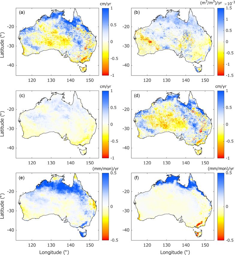
4186                  N. Tangdamrongsub et al.: Development and evaluation of 0.05◦ terrestrial water storage estimates

responding particularly to an increased interest in exploiting      tial resolution and time span receives even more attention at
TWS in interdisciplinary studies (e.g., IPCC, 2007; NASEM,          the local level, where spatial detail down to a few kilometers
2018).                                                              is needed (e.g., Rasmussen et al., 2014; Singh et al., 2015;
   TWS information can be obtained or estimated from                Beamer et al., 2016; Dong et al., 2020).
ground observation networks, satellite measurements, or                On top of the improved spatiotemporal resolutions, the im-
model simulations. Each has different strengths and limi-           proved accuracy of TWS estimates is also a concern in LSM
tations. Ground observations (e.g., soil moisture probe and         developments. As in most environmental modeling systems,
groundwater well) are considered the most reliable, provid-         model outputs are associated with a high degree of uncer-
ing measurements closest to the truth (e.g., Dorigo et al.,         tainty propagated from, e.g., inaccurate meteorological forc-
2013). However, ground observations have high maintenance           ings, imperfect model physics, and ineffective parameter cal-
costs and incomplete coverage. Also, point measurements             ibration. Data assimilation (DA; Reichle et al., 2002; Re-
only reflect information at one location and not necessarily        ichle, 2008) techniques can be employed to improve LSM
the entire region. On the other hand, satellite platforms offer     performance. The approach sequentially updates the model’s
an automated measurement with improved coverage ranging             states using an optimal value computed by combining model
from regional to global (e.g., Tapley et al., 2004; Entekhabi       simulations with observations. A variety of satellite obser-
et al., 2010a). The challenges of using satellite measurements      vations reflecting different TWS components can be assim-
are the coarse spatial resolution and the sensors’ technical        ilated into the system (e.g., Kumar et al., 2014; Dong and
limitations (e.g., penetration depth, cloud/vegetation obstruc-     Crow, 2018). TWS observations from the Gravity Recovery
tion, and background noise). Therefore, its usage is restricted     And Climate Experiment (GRACE) satellite mission (Tap-
to a large region and requires a sophisticated algorithm to re-     ley et al., 2004) offer integrated water column information
trieve TWS variables (Crow et al., 2012; Castellazzi et al.,        that can be used to constrain multiple water storage com-
2016; Tangdamrongsub et al., 2019). In addition, satellite          ponents simultaneously (e.g., Zaitchik et al., 2008; Forman
measurements can be limited by a relatively short period of         et al., 2012; Tangdamrongsub et al., 2015). GRACE DA has
record (e.g., Flechtner et al., 2014; Karthikeyan et al., 2017).    shown positive impacts on most TWS components, including
   TWS components can also be simulated from a land sur-            groundwater (e.g., Girotto et al., 2017; Nie et al., 2019), soil
face model (LSM). The LSM incorporates various land sur-            moisture (Jung et al., 2019), and snow (Kumar et al., 2016).
face physics into complex numerical sequences to allow the             The Community Atmosphere Biosphere Land Exchange
simulation of TWS to be performed at any desired location           model (CABLE; Kowalczyk et al., 2006) is an open-source
and spatiotemporal scale (Pitman, 2003). The LSM can pro-           global LSM developed and updated by the community. CA-
vide a complete suite of TWS components compared with               BLE is a core LSM of the Australian Community Climate
the ground or satellite measurements that can only measure          and Earth System Simulator (ACCESS; Bi et al., 2013;
a single or integrated TWS component (e.g., Tapley et al.,          Kowalczyk et al., 2013) that can be used to simulate water
2004; Entekhabi et al., 2010a). However, due to the limi-           storage and fluxes globally. The model has been regularly
tations of input data, the spatial resolution of many LSMs          updated to incorporate state-of-the-art model physics (e.g.,
is coarse (e.g., > 0.25◦ (∼ 25 km)), which consequently re-         Decker, 2015; Ukkola et al., 2016; Haverd et al., 2018). De-
stricts their application to a large region (e.g., Rodell et al.,   spite its success, CABLE’s spatial scale is currently limited
2004; Alkama et al., 2010; Ke et al., 2012).                        to 0.5◦ (∼ 50 km) due to the 0.5◦ resolution of its parameter
   Efforts to improve the spatial resolution (and time span)        and forcing data sets. This contrasts with other global model
of global TWS estimates have been made in many modeling             developments, where high-resolution versions have already
communities (e.g., Wood et al., 2011; Bierkens et al., 2015;        been developed (e.g., van Dijk et al., 2013a, b; Sutanudjaja
Bierkens, 2015). For instance, Ke et al. (2012) improved the        et al., 2018). CABLE and its inputs must be reconfigured to
resolution of the Community Land Model (CLM) from 0.5◦              increase the spatial detail of TWS estimates for smaller-scale
(∼ 50 km) to 0.05◦ (∼ 5 km) using modified land surface pa-         studies (e.g., 0.01–0.05◦ ). Our effort to increase the study’s
rameters. The World-Wide Water model (W3; van Dijk et               spatial resolution should narrow this development gap and
al., 2013a, b) recently allowed the global TWS variables            has not previously been implemented.
to be estimated at 0.05◦ (∼ 5 km). The European Centre                 This study aims to improve the accuracy, spatial reso-
for Medium-Range Weather Forecasts (ECMWF) Reanaly-                 lution, and time span of CABLE TWS estimates. Our ap-
sis 5 (ERA5) offers global land surface variables at 0.1◦ (∼        proach utilizes only publicly available global data sets, so
9 km) resolution from 1981 to present (see the data availabil-      resulting TWS estimates can be reproduced over any tar-
ity section). A similar effort is also seen in hydrologic model     get region (see the data availability section for the data ac-
development, such as the PCRaster Global Water Balance              cess). The spatial detail of CABLE is improved from 0.5 to
(PCR-GLOBWB; Sutanudjaja et al., 2018), which improves              0.05◦ (∼ 5 km) using high-resolution forcing data (precipita-
the spatial resolution from 30 arcmin (∼ 50 m or ∼ 0.5◦ ) to        tion in particular) and land surface parameters derived from
5 arcmin (∼ 9 km or 0.083◦ ) and extends the time span to           high-resolution maps of soil and vegetation cover. The de-
more than a 50-year period. The enhancement of model spa-           velopment is demonstrated in Australia, where ground ob-

Hydrol. Earth Syst. Sci., 25, 4185–4208, 2021                                        https://doi.org/10.5194/hess-25-4185-2021
N. Tangdamrongsub et al.: Development and evaluation of 0.05◦ terrestrial water storage estimates                            4187

servation networks (e.g., surface soil moisture, groundwa-          2020). Studies relevant to GRACE DA in Australia are sum-
ter, and evapotranspiration) are available to validate the re-      marized in Table 1. Ground observation networks have also
sult. The demonstrated simulation period is 1981–2012, co-          been installed across the continent and continuously monitor
incident with the availability of meteorological forcing data.      the water storage and flux variations. Such data records are
Recent studies have shown success in assimilating GRACE             valuable for validating the accuracy of the model estimates
data into a coarse-scale CABLE version to improve TWS               and remote sensing observations. Details regarding the in situ
and groundwater storage (GWS) estimates in the Goulburn             data used in this study are provided in Sect. 2.3.2.
River catchment and in the North China Plain (Tangdam-
rongsub et al., 2020; Yin et al., 2020). In this study, GRACE       2.2   Model configuration
observations (Luthcke et al., 2013) are also assimilated into
CABLE 0.05◦ (and CABLE 0.5◦ ) to improve the accuracy               In this study, TWS estimates are derived from CABLE. A
of TWS components between 2003 and 2012. Assimilat-                 history of the model’s development can be found in, e.g.,
ing the coarse GRACE observations into a much higher-               Wang et al. (2011), Kowalczyk et al. (2013), Decker (2015),
resolution model is performed using the 3-dimensional en-           and Haverd et al. (2018). Multiple CABLE versions have
semble Kalman smoother (EnKS 3D; Tangdamrongsub et                  been developed since 2003 for different objectives (see the
al., 2017). This approach will reveal whether assimilating          data availability section); CABLE SubgridSoil GroundWa-
GRACE data can benefit a newly developed fine-scale CA-             ter (CABLE-SSGW; Decker, 2015) is considered most suit-
BLE configuration. Our study will perform a thorough in-            able for our use due to its inclusion of comprehensive ter-
vestigation on this issue to address GRACE DA’s benefit on          restrial water storage components and, especially, a ground-
CABLE 0.05◦ .                                                       water module. CABLE is developed using Fortran and can
   The objectives of this paper are (1) to present the devel-       be executed in a Unix environment. The input/output file for-
opment and evaluation of retrospective 0.05◦ TWS estimates          mat follows the NetCDF Climate and Forecast (CF) conven-
and (2) to assess the GRACE DA impact on 0.05◦ CABLE                tion. The model has been used to simulate global TWS at
version, as well as the benefit of assimilating the coarse reso-    0.5◦ spatial resolution using 0.5◦ resolution model param-
lution satellite data into a fine-scale model. This paper is pre-   eters and forcing data (e.g., Decker, 2015; Ukkola et al.,
sented as follows. Section 2 provides the details of the study      2016). The variables used to assess TWS consist of soil mois-
area, model configurations, and data processing. Section 3          ture storage (SMS), snow water equivalent (SWE), canopy
presents the GRACE DA schematic and the statistical metric          storage (CNP), and GWS.
used in the evaluation. Section 4 presents the assessment and          The model parameters of CABLE-SSGW are derived from
validation of the result. Finally, Sect. 5 summarizes the find-     several different sources (Kowalczyk et al., 2006; Wang et
ings of this study and provides a possible direction for future     al., 2011; Decker, 2015). Land use/vegetation type categories
development.                                                        are obtained from the International Geosphere–Biosphere
                                                                    Programme (IGBP) classification from the Moderate Res-
                                                                    olution Imaging Spectroradiometer (MODIS; Friedl et al.,
2     Study area and data                                           2002). Relative volumes of silt, sand, clay, and organic mat-
                                                                    ter in the soil are obtained from the Harmonized World Soil
2.1    Study area                                                   Database (Fischer et al., 2008). The Zobler soil category
                                                                    (Zobler, 1999) is computed empirically from the silt, sand,
This study uses Australia as a case study. Due to its size and      and clay fractions (Oleson et al., 2010). The monthly clima-
geographic location, Australia is influenced by multiple cli-       tology of the leaf area index (LAI) is computed using a repro-
mate drivers (Murphy and Timbal, 2008; Xie et al., 2016)            cessed MODIS LAI product (Yuan et al., 2011). All derived
and experiences episodes of severe droughts and floods (e.g.,       model parameters are resampled to 0.5◦ to match the 0.5◦
van Dijk et al., 2013a). The recent long-term drought, known        model grid space. Comprehensive details of model parame-
as the Millennium Drought (Bond et al., 2008), severely af-         ters can be found in, e.g., Kowalczyk et al. (2006), Wang et
fected industrial and agricultural sectors and has led to a         al. (2011), and Decker (2015).
significant economic loss nationwide (see, e.g., van Dijk et           This study rederives the model parameters and employs
al., 2013a). The need for an accurate prediction of possible        enhanced forcing data to increase the model spatial detail
water scarcity from climate variations motivated the devel-         from 0.5 to 0.05◦ . The vegetation type is derived from the
opment of land surface and hydrology models in Australia,           global land cover climatology using MODIS data (Broxton
e.g., the Australian Water Availability Project (AWAP; Rau-         et al., 2014). The soil map is also derived from the Harmo-
pach et al., 2008), the Australian Water Resources Assess-          nized World Soil Database but at 0.05◦ grid spacing. The
ment – Landscape Model (AWRA-L; van Dijk, 2010), and                0.05◦ monthly climatology LAI is derived from the Global
CABLE (Kowalczyk et al., 2006). Recent work has assimi-             Land Surface Satellite product (GLASS; Xiao et al., 2014).
lated GRACE satellite data into such water models (e.g., Tian       All rederived parameters are shown in Fig. 1. The soil layer
et al., 2017; Schumacher et al., 2018; Tangdamrongsub et al.,       thicknesses, from top to bottom, are set to 1.2, 3.8, 25, 39.9,

https://doi.org/10.5194/hess-25-4185-2021                                        Hydrol. Earth Syst. Sci., 25, 4185–4208, 2021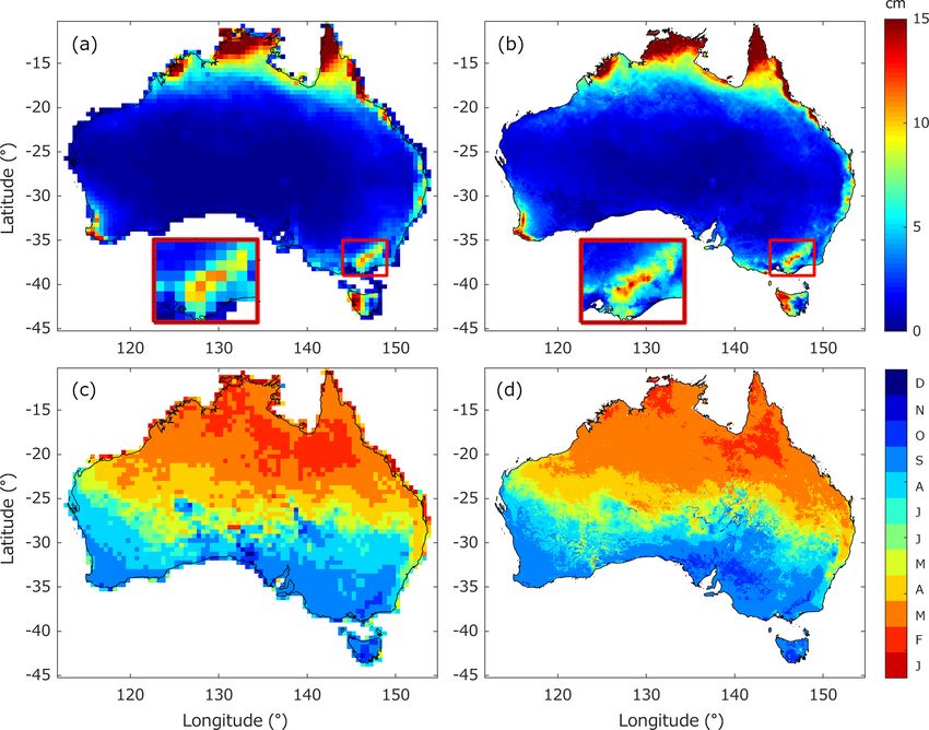
4188 N. Tangdamrongsub et al.: Development and evaluation of 0.05◦ terrestrial water storage estimates
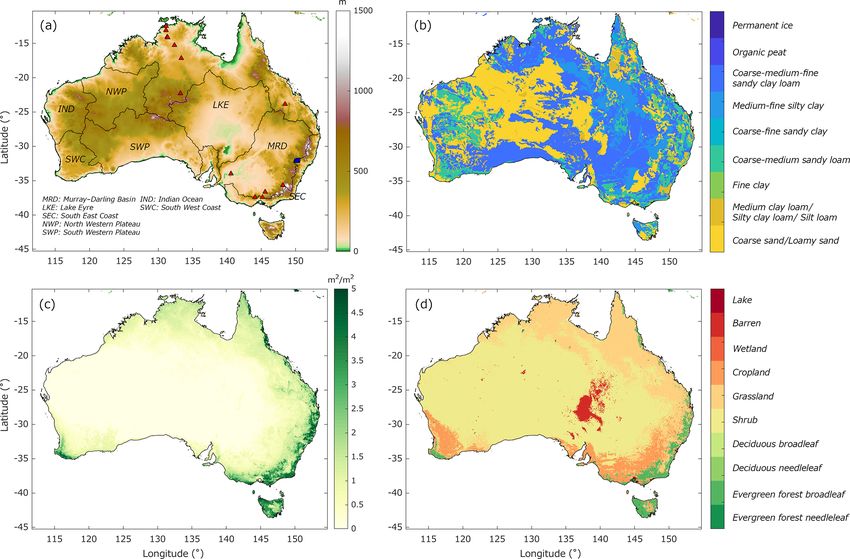
Figure 1. (a) Characteristics of the study area, including elevation, major Australian river basin, and ground observation networks
(FLUXNET – red triangle; the Scaling and Assimilation of Soil Moisture and Streamflow (SASMAS) – blue square). Note that the lo-
cations of groundwater sites can be found in Fig. 14. (a–c) The derived 0.05◦ land cover values for (b) soil class, (c) averaged LAI (used
only for demonstration), and (d) vegetation and land cover types.
107.9, and 287.2 cm, and the unconfined aquifer’s thickness Model simulations are performed between 1981 and 2012
is set to 20 m. The surface soil moisture (SSM; cubic me- (a total of 32 years), given the Princeton forcing data’s avail-
ter per cubic meter, hereafter m3 m−3 ) is defined as the top ability. Similar to McNally et al. (2017), temporal disaggre-
two layers, and the SMS (meters) is computed from all soil gation is applied to CHIRP precipitation data to resample
layers. from 1 d to 3 h, consistent with the Princeton data’s time step.
The CABLE model is forced with precipitation, air tem- The scale factor derived from the 3 h Princeton precipitation
perature, wind speed, humidity, surface pressure, and short- data is used to (temporally) rescale the CHIRPS data. The
wave and longwave downward radiation. For precipitation, characteristics of forcing data and the derived model param-
we use the Climate Hazards Group InfraRed Precipitation eters used in this paper are given in Table 2.
with Station data (CHIRPS; Funk et al., 2015), provided on a In all simulations, initial states are obtained using a 320-
0.05◦ grid. The other forcing variables are provided on a 0.5◦ year spinup, i.e., performing 10 repeated runs between 1981
grid by the high-resolution global data set of meteorological and 2012.
forcings for land surface modeling version 2, Princeton Uni-
versity (Princeton; Sheffield et al., 2006). When performing 2.3 GRACE data
0.5◦ model simulations, the CHIRPS data are spatially aver-
aged to 0.5◦ grid space while other forcing variables main- GRACE is a twin satellite-to-satellite tracking mission de-
tain their intrinsic 0.5◦ resolution. When performing 0.05◦ signed to measure the mean and time-varying components of
model simulations, the coarser-resolution forcing variables the Earth’s gravity field (Tapley et al., 2004). Every month,
are spatially resampled to 0.05◦ model grid space using the GRACE provides a time-varying gravity solution containing
nearest-neighbor interpolation. information about mass redistribution near the Earth’s sur-
face. The monthly gravity change is dominated by a hydrol-
Hydrol. Earth Syst. Sci., 25, 4185–4208, 2021 https://doi.org/10.5194/hess-25-4185-2021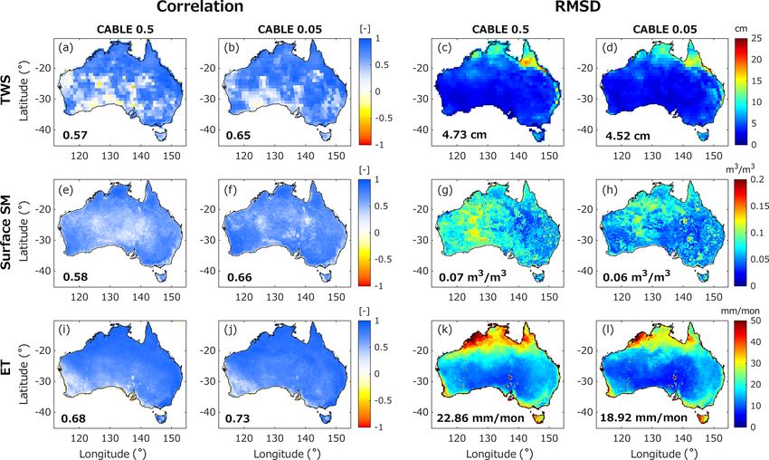
N. Tangdamrongsub et al.: Development and evaluation of 0.05◦ terrestrial water storage estimates                                      4189

Table 1. Relevant studies related to the development of the land surface and hydrology models (with the inclusion of GRACE DA applica-
tions) to estimate TWS in Australia.

           Model                                                 Spatial   Time span     GRACE DA           References
                                                              resolution                 approach
           WaterGAP Global Hydrology Model                          0.5◦   2003–2010     EnKF               Müller Schmied
           (WGHM)                                                                                           (2017); Schumacher et
                                                                                                            al. (2018)
           The World-Wide Water (W3)                                0.5◦   2002–2013     EnKF               Van Dijk et al.
                                                                                                            (2013b); Tian et al.
                                                                                                            (2017)
           World-Wide Water Resources                               0.5◦   2002–2013     Various            Van Dijk (2010);
           Assessment (W3RA)                                                                                Khaki et al. (2017)
           PCRaster Global Water Balance                            0.5◦   2003–2014     EnKS 3D            Sutanudjaja et al.
           (PCR-GLOBWB)                                                                                     (2018); Tangdamrongsub
                                                                                                            et al. (2018)
           NASA’s Catchment Land Surface Model                     0.25◦   2003–2012     EnKS               Koster et al. (2000);
           (CLSM)                                                                                           Li et al. (2019)
           The Australian Water Resources                          0.05◦   2000–2018     Adaptive EnKF      Van Dijk (2010);
           Assessment – Landscape model                                                                     Shokri et al. (2019)
           (AWRA-L)
           The Community Atmosphere Biosphere                      0.05◦   1980–2012     EnKS 3D            This study
           Land Exchange (CABLE) 0.05◦

Table 2. Characteristics of the land cover parameters, meteorological forcing, and remote sensing data used in the development and validation
of CABLE 0.05◦ .

                                          Products                         Grid size   Time          References
                                                                                       interval
             Meteorological               Princeton Forcing data           0.5◦        3h            Sheffield et al. (2006)
             forcing data                 version 2
             Precipitation                Climate Hazards Group            0.05◦       1d            Funk et al. (2015)
                                          InfraRed Precipitation with
                                          Station data (CHIRPS)
             Soil type                    Harmonized World Soil            30 arcsec   n/a           Nachtergaele and Batjes (2012)
                                          Database version 1.2
             Vegetation type              MODIS Land Cover Maps            500 m       n/a           Broxton et al. (2014)
             LAI                          Global Land Surface Satellite    0.05◦       ∼ 8d          Xiao et al. (2014)
                                          (GLASS)
             TWS                          GRACE NASA GSFC                  Irregular   ∼ 1 month     Luthcke et al. (2013)
                                          Mascons
             Soil moisture                European Space Agency –          0.25◦       1d            Dorigo et al. (2017)
                                          Climate Change Initiative
                                          program (ESA CCI)
             Evapotranspiration           Global Land Evaporation          0.25◦       1d            Martens et al. (2017)
                                          Amsterdam Model (GLEAM)

           “n/a” stands for not applicable.

https://doi.org/10.5194/hess-25-4185-2021                                                     Hydrol. Earth Syst. Sci., 25, 4185–4208, 2021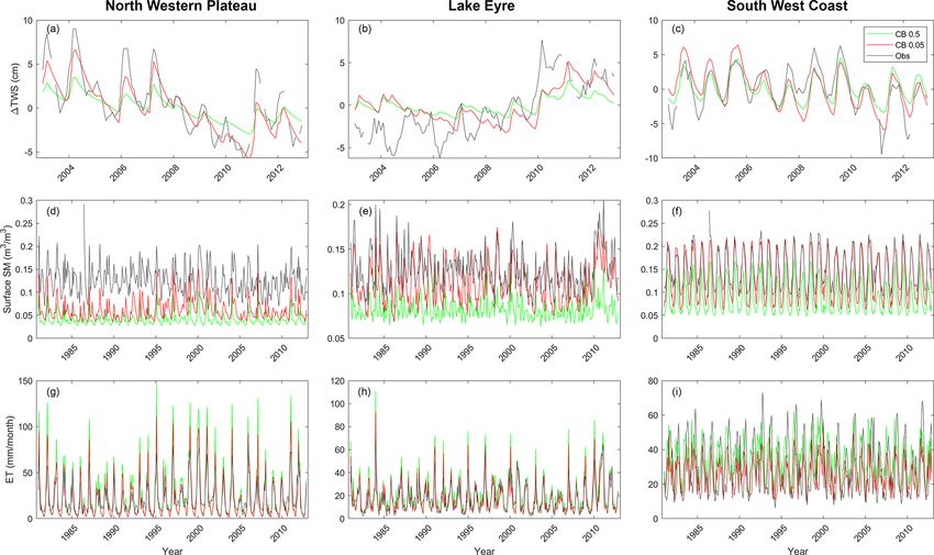
4190                   N. Tangdamrongsub et al.: Development and evaluation of 0.05◦ terrestrial water storage estimates

                                                                       2.4     Evaluation data

                                                                       2.4.1    Satellite-derived products

                                                                       The satellite-derived soil moisture and evapotranspira-
                                                                       tion (ET) data obtained from the European Space Agency
                                                                       Climate Change Initiative program (ESA CCI; Dorigo et al.,
                                                                       2017; Gruber et al., 2019) and the Global Land Evapora-
                                                                       tion Amsterdam Model (GLEAM; Martens et al., 2017) are
                                                                       used to validate the soil moisture and evaporation estimates,
                                                                       respectively. The ESA CCI COMBINED product combines
                                                                       multiple active and passive satellite sensor soil moisture
                                                                       products and provides a near-global daily volumetric soil
                                                                       moisture product at 0.25◦ resolution with ∼ 0.04 m3 m−3
                                                                       accuracy (unbiased root mean square error). The combined
                                                                       product version 4.7 (v04.7) is used in this study. The prod-
                                                                       uct includes approximately eight different satellite observa-
                                                                       tions, including, e.g., SSM/I, AMSR-E, ASCAT, Windsat,
Figure 2. The GRACE GSFC Mascon grid (black rectangles) and
                                                                       and SMOS (see, e.g., Fig. 3 of Dorigo et al. (2017) for
the CABLE 0.05◦ grids (red dots) in Australia. The green inset
shows details of rectangle A. The orange circle B shows the number
                                                                       complete details) during our evaluation period (1981–2012).
of mascon cells inside a ∼ 3◦ radius, which are used to update the     GLEAM is an algorithm that derives the daily global terres-
state variables inside the center mascon (filled orange). Processing   trial evaporation using observations from multiple satellite
details can be found in Sect. 3.1.                                     microwave sensors and reanalysis data sets (Martens et al.,
                                                                       2017). In total, two product variants are available, i.e., the
                                                                       satellite-only and the reanalysis, and the newest release of
ogy signal, making the GRACE product beneficial for var-               the latter (version 3.3a) is used in this study due to its consis-
ious hydrological and geophysical applications (e.g., Klees            tent time span with our evaluation period.
et al., 2008; Mouyen et al., 2018; Rodell et al., 2018; Tap-
ley et al., 2019). Different GRACE solutions have been re-             2.4.2    In situ data
leased, including the mascon solution (e.g., Luthcke et al.,
2008; Rowlands et al., 2010). The mascon approach uti-                 In situ soil moisture, groundwater, and ET measurements are
lizes mass concentration blocks (as a basis function) to de-           obtained from different ground observation networks. The
termine the Earth’s mass variation and is found to provide             daily in situ soil moisture data are obtained from the Scal-
a more accurate TWS estimate compared to the spherical                 ing and Assimilation of Soil Moisture and Streamflow (SAS-
harmonic approach (Rowlands et al., 2010). In this study,              MAS; Rüdiger et al., 2007) network in the southeastern part
the mascon (mass concentration) product from the Goddard               of the Murray–Darling Basin (see Fig. 1). The SASMAS net-
Space Flight Center (GSFC) is used (Luthcke et al., 2013).             work hosts more than 20 measurement sites and provides
The GSFC Mascon product contains monthly TWS vari-                     volumetric soil moisture (θ ; m3 m−3 ) data associated with 0–
ations (1TWS), expressed in equivalent water height (in,               5 cm depth. Only sites with a data record longer than 3 years
e.g., meters). The glacial isostatic adjustment correction is          are used in our analysis.
applied using the ICE6G model (Peltier et al., 2015). The                 The monthly in situ groundwater level data are collected
mascon varies in size and represents the average 1TWS of               from the Australian Bureau of Meteorology through the Aus-
the associated grid cell. The spatial distribution of mascon           tralian Groundwater Explorer. More than 870 000 monitoring
in Australia is shown in Fig. 2. The GSFC Mascon prod-                 bores are distributed across the continent. At each bore, the
uct also provides monthly 1TWS uncertainties, and they                 groundwater level measurement is converted to the ground-
are used to represent the observation error of the individ-            water level variation by removing the long-term mean asso-
ual mascon. In this study, GRACE data are assimilated into             ciated with the entire data record. The bores are excluded
CABLE between January 2003 and December 2012 (due to                   from the analysis if the data record is shorter than 3 years
the availability of GRACE data). To convert monthly 1TWS               or has significant missing data. The groundwater level mea-
into absolute TWS (necessary for the GRACE DA process),                surements are not converted to groundwater storage due to
the temporal mean value of the CABLE-simulated TWS                     the absence of accurate knowledge of specific yield.
from 2003 to 2012 is added to the GSFC Mascon product.                    The in situ ET (i.e., latent heat flux) is obtained from the
This process reconciles the observed long-term mean with               FLUXNET2015 data set (Pastorello et al., 2017). FLUXNET
the model estimates.                                                   is a global network measuring carbon and energy fluxes.
                                                                       More than 20 flux tower sites are distributed across Australia

Hydrol. Earth Syst. Sci., 25, 4185–4208, 2021                                           https://doi.org/10.5194/hess-25-4185-2021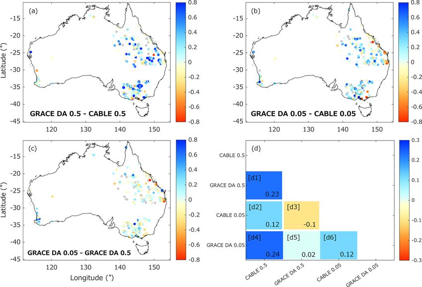
N. Tangdamrongsub et al.: Development and evaluation of 0.05◦ terrestrial water storage estimates 4191
and are associated with different periods (e.g., 2001–2014). ers, canopy storage, snow water equivalent, and groundwater
Only the sites with 3 years of data or longer are used in our storage.
analysis (see site locations in Fig. 1a). In the analysis step, when a GRACE observation is avail-
able, the monthly averaged states (ψ) are related to the
GRACE observations by the following:
3 Methods
d j = Hψ j + j ; ∼ N (0, R), (2)
3.1 Ensemble Kalman smoother (EnKS)
where d j is an m×1 perturbed observation vector containing
The ensemble Kalman smoother (EnKS; Zaitchik et al., the perturbed GRACE mascon for the month of interest, H is
2008) is used to assimilate the GRACE-derived 1TWS into a measurement operator which relates the ensemble state ψ j
the CABLE model. The 3-dimensional EnKS (EnKS 3D) to the vector d j , m is the number of GRACE mascon cells
scheme described in Tangdamrongsub et al. (2017) is used in used in the calculation, and j indicates ensemble index. The
this study for two reasons. First, it accounts for spatial corre- uncertainties in the observations are described by the random
lations in model and observation errors. The latter are highly error , which is assumed to have zero mean and covariance
correlated at neighboring 0.5◦ × 0.5◦ or 0.05◦ × 0.05◦ grid matrix Rm×m . The subscription denotes the dimension of the
cells. Second, EnKS does not require interpolation of the ob- matrix. Note that R is a variance matrix here as only the vari-
servations (as in the ensemble Kalman filter (EnKF); Tang- ance components are provided in the mascon product.
damrongsub et al., 2015) and mitigates the spurious jump in In EnKS 3D, multiple model and observation grid cells
water storage estimates caused by applying updates at the (e.g., inside 300 km radius corresponding to GRACE spatial
end of the month only. The additional computational cost is resolution) are simultaneously used to compute the state up-
small, for handling large covariance matrices and running the date. Figure 2 (see circle B) demonstrates the model and mas-
model twice for each month. con grid cells used in the analysis step to compute the update
The GRACE DA comprises forecast, analysis, and dis- of the center mascon cell (see also Fig. 7 of Tangdamrong-
tributing update steps. The forecast step propagates the sub et al. (2017) for more details). The H matrix is defined
model states forward in time for approximately 1 month. The as follows:
analysis step computes the monthly model state update us-
H=
ing GRACE observations (and uncertainties). The final step 1
(1 1 1 . . . 1)1×nk1 0 ··· 0
reinitializes the ensemble (e.g., initial states and forcing data)
k1
0 1
(1 1 1 . . . 1)1×nk2 ··· 0
k2
and reperforms the forecast step with the DA update (in-
. . . .
,
. . . .
. . . .
crement) distributed evenly throughout the month. Figure 3
0 0 ··· 1
(1 1 1 . . . 1)1×nkm
Pm
km m× i=1 nki
illustrates the concept of the GRACE DA process. Pseu-
(3)
docodes of GRACE DA can be found in the Supplement.
The meteorological forcings and model parameters are where ki is the number of model grid cells inside a mascon i
perturbed using N = 100 ensemble members prior to (see, e.g., rectangle A in Fig. 2 for the distribution of model
GRACE DA processing. Multiplicative white noise is used to grids inside a mascon cell).
perturb the precipitation and shortwave radiation, while addi- The ensemble of the states is stored in a matrix AK×N =
tive white noise is used for the air temperature and model pa- m
P
rameters. The characteristics of the uncertainties are given in (ψ 1 , ψ 2 , ψ 3 , . . ., ψ N ), where K = nki , and the ensem-
i=1
Table 3. Downscaling and upscaling forcing data also cause
ble perturbation matrix is defined as A0 = A − A, where the
errors. In our DA process, when the data are resampled, their
matrix A contains the mean values computed from all ensem-
errors are also adjusted. The relationship between coarse and
ble members. Similarly, the perturbed GRACE observation
fine-scale errors can be expressed as follows:
vector is stored in the matrix Dm×N = (d 1 , d 2 , d 3 , . . ., d N ).
v ! The analysis equation is then expressed as follows:
M X M u 2
u
1 X 2 −φhl
σc = t σf hl exp , (1) Aa = A + 1A = A + K(D − HA), (4)
M h=1 l=1 2φ02
with
where σc and σf represent coarse and fine-scale errors,
−1
(h, l) is the index of a grid cell, M is the number of fine-scale K = Pe HT HPe HT + Re , (5)
grid cells used in resampling, φ is a spherical distance be-
tween grid cells, and φ0 is the considered correlation length where AaK×N represents the updated state vector, 1AK×N is
(e.g., a coarse scale’s grid size). After the perturbation pro- the monthly averaged update from EnKS 3D, and KK×m is
cess, CABLE model states are then propagated for approxi- the Kalman gain matrix. The superscript “T” denotes a trans-
mately 1 month (the forecast step). The state vector consists pose (matrix) operator. The model and observation error co-
of nine model states (n = 9), including six soil moisture lay- variance matrix (Pe )K×K , (Re )m×m are computed as follows:
https://doi.org/10.5194/hess-25-4185-2021 Hydrol. Earth Syst. Sci., 25, 4185–4208, 20214192 N. Tangdamrongsub et al.: Development and evaluation of 0.05◦ terrestrial water storage estimates
Figure 3. The data-processing diagram of the GRACE DA process.
3.2 Assessment metrics and experiment designs
0 0 T
Pe = A (A ) /(N − 1), (6)
3.2.1 Resample approach
T
Re = ϒϒ /(N − 1), (7)
The state estimates are validated against the referenced data
where ϒ contains the measurement error of all ensemble described in Sect. 2.4. As the spatial resolution of the model
members. After the monthly averaged update 1A is ob- estimate and referenced data are different, a spatial resam-
tained, the daily increment (1Ad ) of the update is computed ple is performed before the comparison. The model estimate
by dividing 1A by the total number of days in that month. is resampled to the observation grid space using the nearest-
Note that only 1Ad of the center mascon is saved (see also neighbor gridded interpolation when the model’s resolution
Tangdamrongsub et al., 2017). The processes described in is coarser. Conversely, the estimate is upscaled (spatial aver-
Eqs. (2)–(7) are repeated through all mascon cells to obtain aging) when the model’s resolution is higher. The evaluation
all individual 1Ad in the study domain. Then, the model is conducted at the observation grid cell.
is reinitialized using the previous month’s initial states, and
the simulation is performed again while adding 1Ad to the 3.2.2 Correlation and root mean square difference
model initial states daily (the distributing update step). The
DA process is performed until the last month of the study The agreement between the estimated variable and the in situ
period (December 2012). data is assessed using the Pearson correlation coefficient (ρ)
and the root mean square difference (RMSD). At a particular
grid cell, ρ is calculated as follows:
Hydrol. Earth Syst. Sci., 25, 4185–4208, 2021 https://doi.org/10.5194/hess-25-4185-2021N. Tangdamrongsub et al.: Development and evaluation of 0.05◦ terrestrial water storage estimates 4193
Table 3. Perturbation settings associated with the meteorological forcing data and model parameters. The comprehensive description of
model parameters can be found in, e.g., Decker (2015) and Ukkola et al. (2016). The spatial correlation error is also applied to forcing data
(fourth column). The correlation length of the 0.5 and 0.05◦ CABLE model (C05 and C005) is determined based on covariance analysis (see
Sect. 3.2.4).
Forcing/ Description Perturbation Spatially correlated Standard
parameter type (correlation length) deviation
variables
Meteorological forcings
Rainf Precipitation Multiplicative Yes 10 % of the
(C05 = 0.7◦ ; C005 = 0.3◦ ) nominal value
Tair Air temperature Additive Yes 2 ◦C
(C05 = 2.1◦ ; C005 = 2.1◦ )
SW Shortwave radiation Multiplicative Yes 10 % of the
(C05 = 2.3◦ ; C005 = 2.3◦ ) nominal value
Model parameters
fclay , fsand , The fraction of clay, Multiplicative No 10 % of the
fsilt sand, and silt nominal value
fsat The fraction of the grid Additive No 10 % of the
cell that is saturated nominal value
qsub The maximum rate of Additive No 10 % of the
subsurface drainage nominal value
assuming a fully
saturated soil column
fp Tunable parameter Additive No 10 % of the
controlling drainage nominal value
speed
ω = 2π/T , (11)
ρ = E[(y − y)(x − x)]/ σy σx , (8)
where the y vector contains the model estimates, the x vector where the t vector contains time, and T is an annual period.
contains the validation data (observations), E[ ] is the expec- The annual amplitude (A) and phase (ϕ) are computed as
tation operator, and (y, x), and (σy , σx ) are the mean and follows:
p
standard derivations of y and x, respectively. The RMSD is A = c2 + d 2 , (12)
computed as follows:
ϕ = arctan2 (c, d). (13)
qX
RMSD = (y − x)2 /L, (9) 3.2.4 Spatial resolution
where L denotes the length of the time series. Spatial resolution is defined as the minimum distance at
which two signals of equal magnitude can be separated.
3.2.3 Long-term trend and seasonal variations The spatial resolution can be determined from the empirical
(and isotropic) covariance function (C) computed as follows
The long-term trend, annual amplitude, and phase of the time (Tscherning and Rapp, 1974):
series are computed using the least-squares adjustment asso- X
ciated with five parameters, offset (a), long-term trend (b), C (φhl ) = ph pl /nhl , (14)
annual variation (c, d), and semi-annual variation (e, f ). A
time series (y) at a particular grid cell can be expressed as where (ph , pl ) are vectors containing data points (h, l) asso-
follows: ciated with the spherical distance φhl , and nhl is the number
of data pairs considered in the calculation. The spatial reso-
y = a + bt + c sin ωt + d cos ωt + e sin 2ωt + f cos 2ωt, (10) lution (or correlation length of the covariance function) is de-
fined in this study as being the distance ψ at which C(φ = 0)
https://doi.org/10.5194/hess-25-4185-2021 Hydrol. Earth Syst. Sci., 25, 4185–4208, 20214194 N. Tangdamrongsub et al.: Development and evaluation of 0.05◦ terrestrial water storage estimates
January 1981 to December 2012. After obtaining TWS esti-
mates, the TWS annual amplitude and phase are computed
using Eqs. (12) and (13) and are shown in Fig. 5. Both CA-
BLE versions have similar spatial features, but more local-
ized and much finer details are seen in the CABLE 0.05◦ sim-
ulation than in the CABLE 0.5◦ simulation. A clear differ-
ence in annual amplitude is shown over the Yarra Ranges and
the Alpine National Park (compare Fig. 5a vs. Fig. 5b insets).
CABLE 0.05◦ provides greater details of the 1TWS spatial
distribution, and the annual amplitude is approximately 30 %
higher than it is in the coarse-scale version. Differences in
spatial details are also seen in the phase estimates (see Fig. 5c
vs. Fig. 5d).
The spatial resolutions can be quantitatively determined
Figure 4. The concept used to determine spatial resolution (corre- using the empirical covariance function, Eq. (14), described
lation length). The spatial resolution is defined to be the spherical in Sect. 3.2.4. The covariance function is computed for each
distance φ at which the 0 km covariance (or normalized covariance), month’s TWS estimates using all grid points in Australia.
C(φ = 0) decreases by half. Figure 6 shows the averaged spatial resolution (correlation
length) of CABLE 0.5◦ and CABLE 0.05◦ for each month
between 1981 and 2012. The CABLE 0.5◦ simulations have
decreases by half. The diagram in Fig. 4 illustrates how this a spatial resolution of ∼ 50 km, consistent with the grid
correlation length is determined. size of the input 0.5◦ CABLE parameters and forcing data.
Larger correlation lengths are found during the rainy seasons
3.2.5 Case studies (January–April in the north and August–November in the
south) and during the dry season (e.g., June). Soil moisture
This paper uses four case studies to quantify the effect of
and aquifer storage increase during the wet seasons, leading
different model grid sizes and GRACE DA. The case studies
to more uniform (and smoother) spatial moisture features.
are described as follows:
Similar uniformity can also be observed during the dry sea-
1. CABLE 0.5◦ – CABLE model simulations at 0.5◦ grid son. At the beginning of the wet season, scattered rainfall in
size without GRACE DA; part of the continent likely causes a gradient between dry/wet
areas, resulting in smaller correlation lengths. It is notewor-
2. CABLE 0.05◦ – CABLE model simulations at 0.05◦ thy that our analysis only explains the overall temporal pat-
grid size without GRACE DA; tern of continental correlation lengths. The temporal pattern
may also be affected by the local TWS wet/dry features or by
3. GRACE DA 0.5◦ – CABLE model simulations at 0.5◦
the spatial distribution of model parameters.
grid size with GRACE DA;
The use of CABLE 0.05◦ significantly improves the spa-
4. GRACE DA 0.05◦ – CABLE model simulations at tial resolution by about a factor of 2 to 3. Note, again, that
0.05◦ grid size with GRACE DA. the spatial resolution of CABLE 0.05◦ presented in Fig. 6 re-
flects the continental averaged value while the finer (higher)
It is noteworthy that the 0.5 or 0.05◦ represents the CABLE spatial resolution is observed in the individual river basin (not
grid size, which may differ from the spatial resolution. The shown).
term “spatial resolution”, as used in this paper, refers to the
determined resolution computed from Sect. 3.2.4. 4.1.2 Assessment of long-term TWS variations
This study’s time span allows for an assessment of overall
4 Results and discussions
trends and decadal variations in TWS estimates. The long-
4.1 Estimation of TWS components from CABLE term trends of water balance states and fluxes from CABLE
simulations (without GRACE DA) 0.05◦ between 1981 and 2012 are shown in Fig. 7. A strong
relationship between components is observed, particularly in
4.1.1 Improvement in spatial resolution the storage components (Fig. 7a–d). The TWS and GWS
(Fig. 7a and d) have very similar spatial patterns, where a
The resolution improvements can be seen by comparing CA- wetting trend is observed in the northern region, the Indian
BLE 0.5◦ TWS estimates against those from CABLE 0.05◦ . Ocean basin, and the western part of the Murray–Darling
Both are open-loop (OL) simulations, meaning the model is Basin (see Fig. 1a for the basin’s location), and a drying
run without data assimilation. The simulation period is from trend is seen in the central part of the continent, the South
Hydrol. Earth Syst. Sci., 25, 4185–4208, 2021 https://doi.org/10.5194/hess-25-4185-2021N. Tangdamrongsub et al.: Development and evaluation of 0.05◦ terrestrial water storage estimates 4195
Figure 5. Annual amplitude (a, b) and phase (c, d) of the TWS estimates computed from CABLE 0.5◦ (a, c) and CABLE 0.05◦ (b, d).
The insets in (a) and (b) show details in southeastern Australia. The phase exhibits the timing when TWS reaches the maximum value (with
respect to the beginning of the year). The unit of the phase is a calendar month, e.g., January (J) or December (D).
SSM trends (Fig. 7e vs. Fig. 7b), which may be explained by
ET pulling moisture from SSM stores. The long-term trend
of the total runoff is in line with the TWS/GWS, increas-
ing in the north and decreasing in the southeastern region
and Tasmania (e.g., Fig. 7f vs. Fig. 7a). In the northern re-
gion, the soil moisture or aquifer is likely saturated due to a
wet climate, with more significant annual rainfall (than the
south) by about a factor of 5 (not shown). Such a condition
leads to a greater magnitude of root zone moisture, ground-
water recharge, and surface runoff variations. The opposite
scenario is observed in the southeastern region, where the
Figure 6. Monthly average spatial resolutions (correlation lengths) depleted TWS/GWS (induced by droughts) likely reduces
of the TWS estimates derived from CABLE 0.5◦ and CABLE 0.05◦ runoff generation, resulting in a negative runoff trend.
in Australia between 1981 and 2012. Regional water balance components can also be analyzed
at interannual and decadal timescales. Figure 8 shows the
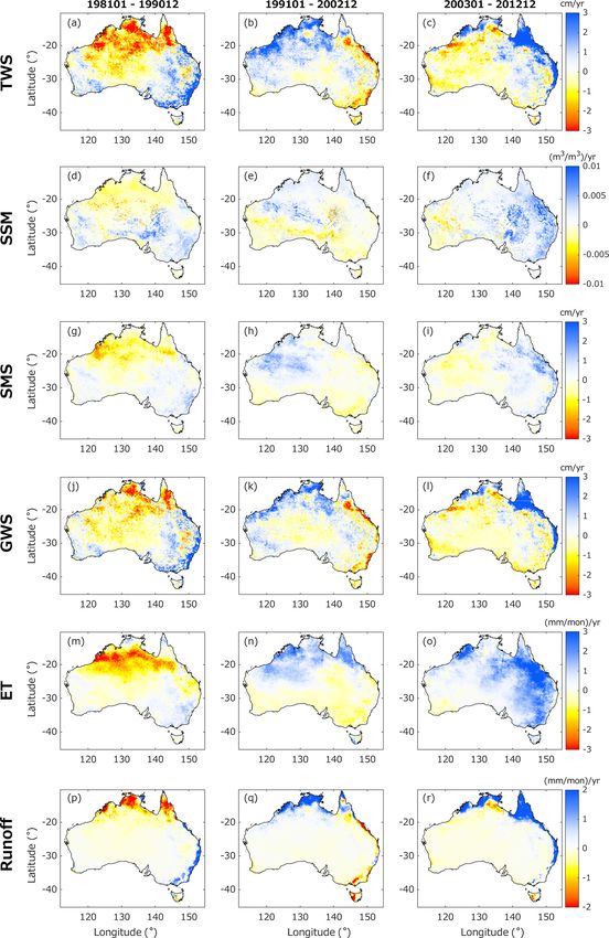
trends of water balance components in 3 different decades,
West Coast basin, and several parts of the Murray–Darling i.e., 1981–1990, 1991–2002, and 2003–2012. The long-term
Basin. The similarity between the TWS and GWS (both spa- trends are not monotonic. In other words, there are no “al-
tially and in magnitude) indicates that GWS is a primary ways dry” or “always wet” regions observed between 1981
driver of the TWS trend in Australia. By contrast, soil mois- and 2012. Reversals between increasing and decreasing
ture stores show different spatial patterns; increases in soil trends are apparent in all components. For example, north-
moisture are also found in the central and western parts of ern and western Australia experience a drying trend be-
the continent (Fig. 7c). The SMS generally accommodates tween 1981 and 1990 (Fig. 8a) and recover between 1991
a large portion of the seasonal variation in water storage in and 2002 (Fig. 8b) after continuously receiving increased
Australia (see Sect. 4.2), but its role in the long-term trend rainfall (not shown). The region experiences another drought
is marginal – smaller than that of the GWS by about a fac- episode (van Dijk et al., 2013a) in the first half of the 2000s,
tor of 2. ET trend estimates show a similar spatial pattern to
https://doi.org/10.5194/hess-25-4185-2021 Hydrol. Earth Syst. Sci., 25, 4185–4208, 20214196 N. Tangdamrongsub et al.: Development and evaluation of 0.05◦ terrestrial water storage estimates
Figure 7. Long-term trends computed from CABLE 0.05◦ between January 1981 and December 2012, showing the (a) terrestrial wa-
ter storage (TWS), (b) surface (volumetric) soil moisture (SSM), (c) total soil moisture storage (SMS), (d) groundwater storage (GWS),
(e) evapotranspiration (ET), and (f) total runoff.
causing decreased water storage between 2003 and 2012 mates, and that this can offer a more reliable assessment of
(Fig. 8c). A similar reversal is also seen in the eastern re- regional water resources and climate variations.
gions, with wetting in 1981–1990, drying in 1991–2002, and
wetting again in 2003–2012 (Fig. 8a–c). 4.1.3 Comparison with the satellite products
Without such a long record, assessment of water resources
may have limited reliability. For instance, based only on the
TWS, SSM, and ET estimates are compared with satellite
∼ 10-year period of GRACE observations, it is difficult to
data from GRACE, ESA CCI, and GLEAM, respectively
determine whether the negative TWS trend in western Aus-
(see Sect. 2.2 and 2.3 for each product’s description). Note
tralia (e.g., Fig. 8c; see also Fig. 11d) is caused by anthro-
that the remote sensing products may contain biases (caused
pogenic or natural processes (e.g., Richey et al., 2015). Evap-
by, e.g., background model and processing algorithm) and
oration or runoff after the extremely wet conditions prior
do not necessarily represent the truth. (Ground truth vali-
to 2002 may also produce a similar decreasing trend (e.g.,
dation is performed in Sect. 4.3.) The intercomparison per-
van Dijk et al., 2011; Munier et al., 2012). By assessing
formed in this section is only to assess the consistency be-
the historical TWS time series of the North Western Plateau
tween two independent estimates, i.e., model and satellite.
basin obtained from CABLE 0.05◦ (Fig. 9), the observed
The CABLE estimate is rescaled to the satellite product’s
negative trend is more likely governed by a decadal cycle of
grid before comparison, as described in Sect. 3.2.1. Fig-
drought and recovery. This approach demonstrates that there
ure 10 shows the correlation and RMSD estimates between
is clear value in utilizing a longer time span of TWS esti-
CABLE 0.5◦ and CABLE 0.05◦ results and the evaluated
Hydrol. Earth Syst. Sci., 25, 4185–4208, 2021 https://doi.org/10.5194/hess-25-4185-2021N. Tangdamrongsub et al.: Development and evaluation of 0.05◦ terrestrial water storage estimates 4197 Figure 8. Similar to Fig. 7 but the trends are associated with three different periods, i.e., 1981–1990 (a, d, g, j, m, p), 1991– 2002 (b, n, h, k, n, q), and 2003–2012 (c, f, i, l, o, r). https://doi.org/10.5194/hess-25-4185-2021 Hydrol. Earth Syst. Sci., 25, 4185–4208, 2021
4198                  N. Tangdamrongsub et al.: Development and evaluation of 0.05◦ terrestrial water storage estimates

                                                                    lite data. The use of coarse-resolution forcing data (e.g., pre-
                                                                    cipitation) could also explain the small TWS amplitude ob-
                                                                    served in CABLE 0.5◦ . Coarse-scale forcing data averages
                                                                    local precipitation signals over a larger area than the finer-
                                                                    resolution forcing data does, resulting in a smaller amplitude.

                                                                    4.2   The impact of GRACE DA

                                                                    GRACE observations are assimilated into the CABLE 0.5◦
                                                                    and CABLE 0.05◦ models (called GRACE DA 0.5◦ and
                                                                    GRACE DA 0.05◦ , respectively) between January 2003 and
                                                                    December 2012 (due to the availability of meteorological
Figure 9. The TWS estimates of the Sandy Desert basin obtained      forcing and GRACE data). The basin-averaged TWS esti-
from CABLE 0.05◦ between January 1981 and December 2012.            mates from CABLE with and without GRACE DA are shown
The long-term trend estimates (centimeters per year) in different   in Fig. 12, alongside the GRACE observations themselves.
periods are given. The blue highlight indicates the GRACE period    In most basins, apparent disagreements between the open-
(January 2003–December 2012).                                       loop estimates and the GRACE observations suggest the cur-
                                                                    rent CABLE models’ limited accuracy. After assimilating
                                                                    GRACE into the models, the estimates (GRACE DA 0.5◦
satellite data. On average, both CABLE results are in good          and GRACE DA 0.05◦ ) move toward the GRACE obser-
agreement with the satellite products, with correlation values      vations. The positive impact of GRACE DA on the basin-
greater than 0.55 (see Fig. 10a, b, e, f, i, j). CABLE 0.05◦        averaged TWS estimates is similar regardless of the model
shows a more robust agreement with satellite-derived vari-          spatial resolutions. This likely reflects the nature of GRACE
ables than CABLE 0.5◦ does; correlation values with TWS,            observations that provide integrated water storage informa-
SSM, and ET are 14 %, 14 %, and 7 % higher (respectively)           tion at the continental or basin scale (Tapley et al., 2004).
in the former simulations than in the latter. Similar improve-      However, it should be noted that the GRACE DA applica-
ments are also observed in the RMSD evaluations, where              tion does not degrade the spatial resolution of the model. The
CABLE 0.05◦ provides smaller RMSD values than CABLE                 offline analysis shows that the average correlation length of
0.5◦ by 4 % (TWS), 14 % (SSM), and 17 % (ET). CABLE                 GRACE DA 0.5◦ and GRACE DA 0.05◦ remain the same
0.05◦ reduces the RMSD of the SSM estimate to as low as             as that of CABLE 0.5◦ and CABLE 0.05◦ , respectively (not
∼ 0.03 m3 m−3 , e.g., over the South West Coast and Lake            shown). The EnKS 3D scheme exploits the spatially corre-
Eyre basins, and the average RMSD value in Australia is             lated information from the high-resolution model to disag-
∼ 0.06 m3 m−3 . It is worth noting that the average unbiased        gregate the coarse-scale observations into a finer grid space,
RMSD value (Entekhabi et al., 2010b) is 0.037 m3 m−3 (not           resulting in the preservation of the model’s intrinsic resolu-
shown), in line with the accuracy of the CCI product (see,          tion. The impact of GRACE DA is also observed in water re-
e.g., Table 1 of Dorigo et al., 2017).                              distribution within the water storage components. Figure 13
   The improved agreement between CABLE 0.05◦ estimates             shows the contributions of four different water storage com-
and the satellite products is also seen in the temporal vari-       ponents (SMS, GWS, SWE, and CNP) to TWS in different
ation (Fig. 11). Compared with the CABLE 0.5◦ results,              basins before (CABLE 0.05◦ ; Fig. 13a) and after the appli-
CABLE 0.05◦ increases the dynamic range of the TWS es-              cation of GRACE DA (GRACE DA 0.05◦ ; Fig. 13b). The
timates in most basins, leading to closer alignment with            contribution is calculated as a percent of the annual ampli-
GRACE observations (Fig. 11a–c). Similar increases in the           tude of TWS fluctuations. In CABLE 0.05◦ (Fig. 13a), the
agreement are also observed in the CABLE 0.05◦ SSM and              SMS is a major contributor to more than 90 % of the TWS
ET estimates (Fig. 11d–i). The observed improvement may             variation (i.e., annual amplitude). The GWS contribution is
be attributed, in part, to the rederived model parameters. For      only ∼ 10 %. After applying GRACE DA (Fig. 13b), the
example, in the North Western Plateau basin, CABLE 0.05◦            contribution of the GWS is significantly increased. It dom-
uses a ∼ 17 % higher area-averaged sand fraction than CA-           inates the entire water column in several basins (e.g., In-
BLE 0.5◦ does, which allows faster infiltration/drainage in         dian Ocean, Lake Eyre, North West Plateau, and South West
the storage compartments, leading to greater dynamic ranges         Plateau). This behavior reflects the nature of GRACE in that
of TWS and SSM variations (see Fig. 11a and d). Conse-              the groundwater provides a majority of the seasonal changes
quently, the ET estimate is decreased as a response to in-          to terrestrial water mass. GRACE DA has been shown to
creased water storage following the water balance equation          significantly affect GWS in previous studies (e.g., Girotto
(Fig. 11g). Similar mechanisms are also observed in the Lake        et al., 2016; Tangdamrongsub et al., 2018; Li et al., 2019).
Eyre and South West Coast basins, where the improved pa-            The contributions of the SWE and CNP components are neg-
rameterization leads to improved agreement with the satel-          ligible across Australia, and the impact of GRACE DA on

Hydrol. Earth Syst. Sci., 25, 4185–4208, 2021                                        https://doi.org/10.5194/hess-25-4185-2021
N. Tangdamrongsub et al.: Development and evaluation of 0.05◦ terrestrial water storage estimates 4199 Figure 10. The comparison between CABLE 0.5◦ and CABLE 0.05◦ estimates and different remote sensing products in terms of correlation coefficient (a, b, f, i, j) and root mean square difference (RMSD; c, d, g, h, k, l). The terrestrial water storage (TWS; a–d), surface soil moisture (SSM; e–h), and evapotranspiration (ET; i–l) are compared with GRACE, ESA CCI, and GLEAM products, respectively. The averaged statistical values (over Australia) associated with each comparison are also given. Figure 11. The change in terrestrial water storage (1TWS; a–c), surface soil moisture (SSM; d–f), and evapotranspiration (ET; g–i) estimated from CABLE 0.5◦ (CB0.5), CABLE 0.05◦ (CB0.05), and remote sensing observations (Obs) over three different river basins, i.e., North Western Plateau (a, d, g), Lake Eyre (b, e, h), and South West Coast (c, f, i), between 1981 and 2012. The remote sensing observations used for comparison are GRACE (TWS), ESA CCI (SSM), and GLEAM (ET). https://doi.org/10.5194/hess-25-4185-2021 Hydrol. Earth Syst. Sci., 25, 4185–4208, 2021
4200                  N. Tangdamrongsub et al.: Development and evaluation of 0.05◦ terrestrial water storage estimates

Figure 12. The TWS estimates from case studies CABLE 0.5◦ , CABLE 0.05◦ , GRACE DA 0.5◦ , and GRACE DA 0.05◦ in various river
basins between 2003 and 2012. The GRACE observation is also displayed for comparison. Full descriptions of the case studies are given in
Sect. 3.2.5.

them is trivial. Similar changes to TWS contributions are also        consistent with the GRACE DA period. Figure 14 shows
observed between CABLE 0.5◦ and GRACE DA 0.5◦ (not                    the validation of GWS estimates between GRACE DA and
shown). It is noted that Figs. 12 and 13 only present the im-         OL simulations (DA minus OL). A positive value indicates
pact of GRACE DA on storage components and do not assess              improvement, while a negative value represents degradation.
the accuracy of either version. The accuracy of the OL and            A significance test is performed at the 0.05 level based on the
DA models is quantified in Sect. 4.3.                                 Fisher Z transformation test for correlation coefficients (Za-
                                                                      itchick et al., 2008). The average change in correlation value
4.3    Validation with in situ data                                   across all in situ data sites is shown in Fig. 14d. Values that
                                                                      failed the significant test are excluded from the averaging.
In situ data from three different ground networks (see                   We first analyze the impact of GRACE DA on the GWS
Sect. 2.3.2) are used to validate the GWS, ET, and SSM es-            estimates of CABLE 0.5◦ and CABLE 0.05◦ (Fig. 14a
timates. Validation is conducted by quantifying the change            and b). A greater correlation improvement is observed when
in correlation values between simulations and observations            GRACE DA is applied to the 0.5◦ model, which increases
when one model is used in place of another. The valida-               the average correlation value by 0.23 (Fig. 14d1). When
tion period is between January 2003 and December 2012,

Hydrol. Earth Syst. Sci., 25, 4185–4208, 2021                                           https://doi.org/10.5194/hess-25-4185-2021
N. Tangdamrongsub et al.: Development and evaluation of 0.05◦ terrestrial water storage estimates 4201
but positive impact on SSM estimates, improving correla-
tion with observations by ∼ 1 %. The small impact is at-
tributed to limited GRACE sensitivity. GRACE is sensitive to
the low-frequency variation (originated from deeper stores)
and cannot effectively capture SSM, which is dominated
by a high-frequency signal (e.g., precipitation). As a result,
GRACE DA is found to have a minor (or negative) impact on
the top soil component in most GRACE DA studies (e.g., Li
et al., 2012; Tian et al., 2017; Tangdamrongsub et al., 2020).
The small impact on SSM estimates also agrees with Jung et
al. (2019), who observed GRACE DA’s small (or negative)
impact over dry regions in West Africa.
For ET (Fig. 15b), CABLE 0.05◦ exhibits a more im-
proved correlation with observations (by ∼ 5 %) than CA-
BLE 0.5◦ does. The inclusion of GRACE DA also slightly
Figure 13. Contributions of different storage components (total soil improves correlation values over the associated OL model
moisture storage – SMS; groundwater storage – GWS; canopy stor- versions. Greater improvement (by ∼ 2 %) is seen between
age – CNP; and snow water equivalent – SWE) to the TWS esti- CABLE 0.5◦ and GRACE DA 0.5◦ than between CABLE
mates computed from CABLE 0.05◦ (a) and GRACE DA 0.05◦ (b) 0.05◦ and GRACE DA 0.05◦ . As with SSM, the small
in different river basins. The full names of the river basins are given improvement of ET is likely attributable in part to small
in Fig. 1a. Contributions of CNP + SWE are negligible in both pan-
GRACE DA updates (caused by the limited GRACE sensitiv-
els.
ity to high-frequency surface fluxes). The SSM is a primary
moisture source for ET, so a trivial change in SSM leads to a
similarly small change in ET.
GRACE DA is applied to the 0.05◦ model (Fig. 14b), the av-
erage correlation value improves by 0.12 (Fig. 14d6), which
is ∼ 50 % less than in the 0.5◦ model. 5 Conclusion
When comparing the two OL runs (CABLE 0.5◦ vs. CA-
BLE 0.05◦ ), the GWS estimate from CABLE 0.05◦ has a This study enhances the spatial resolution and time span
higher correlation value by 0.12 (see Fig. 14d2). This anal- (> 30 years) of regional TWS estimates using the CABLE
ysis indicates that the lower correlation improvement seen LSM, high-resolution land cover maps and forcing data, and
between CABLE 0.05◦ and GRACE DA 0.05◦ is unlikely GRACE DA application. By improving the model parame-
caused by the reduced impact of GRACE DA on the high- ter and forcing data (without GRACE DA), the developed
resolution model. Rather, it is a result of CABLE 0.05◦ hav- CABLE 0.05◦ model shows clear improvements in the accu-
ing better accuracy to start with. GRACE DA tends to pro- racy of water balance component estimates (e.g., soil mois-
vide the same information to both 0.5 and 0.05◦ models. Still, ture, groundwater, and evapotranspiration) when compared
GRACE DA 0.05◦ exhibits the best correlation with in situ with in situ and independent satellite data. The 0.05◦ model
data, ∼ 0.02 higher than GRACE DA 0.5◦ (Fig. 14c and d5). also improves the spatial resolution by a factor of 2 to 3 over
While GWS estimates from both CABLE 0.5◦ and CABLE the 0.5◦ version. The extended time span provides insightful
0.05◦ improve with GRACE DA, we find that GRACE DA information for long-term assessment of regional water re-
0.5◦ (DA) shows a higher correlation value than CABLE sources and climate variability. The enhanced model param-
0.05◦ (OL) by 0.1 (see Fig. 14d3). This indicates that im- eterization is found to play a significant role in the improved
proving model state estimates via DA is more effective than TWS estimates. Incorporating GRACE DA into the model
improving model parameters via increased resolution. De- leads to further improvements in TWS component estimates.
spite different study areas, LSMs, and validation data, our The positive impact of GRACE DA is found in the deep stor-
finding is in line with, e.g., Girotto et al. (2017) and Nie et age component (e.g., GWS), while the impact on the surface
al. (2019), who also found a significant impact of GRACE components and flux estimates (i.e., SSM and ET) is trivial.
DA on GWS components. Of the four case studies investigated here, the most accurate
SSM and ET estimates are validated against ground mea- simulation uses CABLE 0.05◦ with GRACE DA.
surements from SASMAS and Ozenet, respectively. Corre- The enhanced CABLE model resolution developed in this
lation coefficients between the case study simulations and study relies on improved parameter and forcing data. The
observation networks are summarized in Fig. 15. For SSM land surface physics remains unchanged. The workflow can
(Fig. 15a), CABLE 0.05◦ exhibits slightly improved cor- be adopted for other CABLE repositories or different LSMs
relation with observations (by ∼ 0.6 %) than CABLE 0.5◦ with only slight modifications, e.g., number of soil or vege-
does. The addition of GRACE DA also shows a small tation types. This means TWS estimates can be reproduced
https://doi.org/10.5194/hess-25-4185-2021 Hydrol. Earth Syst. Sci., 25, 4185–4208, 2021You can also read