Effects of heterogeneous reactions on tropospheric chemistry: a global simulation with the chemistry-climate model CHASER V4.0 - GMD
←
→
Page content transcription
If your browser does not render page correctly, please read the page content below
Geosci. Model Dev., 14, 3813–3841, 2021
https://doi.org/10.5194/gmd-14-3813-2021
© Author(s) 2021. This work is distributed under
the Creative Commons Attribution 4.0 License.
Effects of heterogeneous reactions on tropospheric chemistry: a
global simulation with the chemistry–climate model CHASER V4.0
Phuc T. M. Ha1 , Ryoki Matsuda1 , Yugo Kanaya2 , Fumikazu Taketani2 , and Kengo Sudo1,2
1 Graduate School of Environmental Studies, Nagoya University, Nagoya, 464-8601, Japan
2 Research Institute for Global Change, JAMSTEC, Yokohama, 236-0001, Japan
Correspondence: Phuc T. M. Ha (hathiminh.phuc@gmail.com)
Received: 6 October 2020 – Discussion started: 5 November 2020
Revised: 18 May 2021 – Accepted: 24 May 2021 – Published: 24 June 2021
Abstract. This study uses a chemistry–climate model increasing loss rate. However, this positive tendency turns to
CHASER (MIROC) to explore the roles of heterogeneous reduction at higher rates (> 5 times). Our results demonstrate
reactions (HRs) in global tropospheric chemistry. Three dis- that the HRs affect not only polluted areas but also remote
tinct HRs of N2 O5 , HO2 , and RO2 are considered for sur- areas such as the mid-latitude sea boundary layer and upper
faces of aerosols and cloud particles. The model simu- troposphere. Furthermore, HR(HO2 ) can bring challenges to
lation is verified with EANET and EMEP stationary ob- pollution reduction efforts because it causes opposite effects
servations; R/V Mirai ship-based data; ATom1 aircraft between NOx (increase) and surface O3 (decrease).
measurements; satellite observations by OMI, ISCCP, and
CALIPSO-GOCCP; and reanalysis data JRA55. The hetero-
geneous chemistry facilitates improvement of model perfor-
mance with respect to observations for NO2 , OH, CO, and 1 Introduction
O3 , especially in the lower troposphere. The calculated ef-
fects of heterogeneous reactions cause marked changes in Heterogeneous reactions (HRs) on the surfaces of atmo-
global abundances of O3 (−2.96 %), NOx (−2.19 %), CO spheric aerosols and cloud droplets are regarded as playing
(+3.28 %), and global mean CH4 lifetime (+5.91 %). These crucial roles in atmospheric chemistry. They affect ozone
global effects were contributed mostly by N2 O5 uptake onto (O3 ) concentrations in various pathways via the cycle of odd
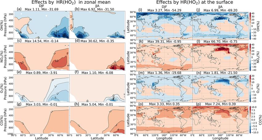
aerosols in the middle troposphere. At the surface, HO2 up- hydrogen (HOx ) and nitrogen oxides (NOx ) (Jacob, 2000).
take gives the largest contributions, with a particularly sig- Tropospheric ozone, an important greenhouse gas, causes
nificant effect in the North Pacific region (−24 % O3 , +68 % damage to human health, crops, and ecosystem productivity
NOx , +8 % CO, and −70 % OH), mainly attributable to its (Monks et al., 2015). Although tropospheric O3 was recog-
uptake onto clouds. The RO2 reaction has a small contribu- nized as a critical oxidant species, its global distribution has
tion, but its global mean negative effects on O3 and CO are not been adequately captured to date because of the limited
not negligible. In general, the uptakes onto ice crystals and number of observations. Whereas many sites in the heavily
cloud droplets that occur mainly by HO2 and RO2 radicals polluted regions of eastern Asia show ozone increases since
cause smaller global effects than the aerosol-uptake effects 2000 (Liu and Wang, 2020), many sites in other regions show
by N2 O5 radicals (+1.34 % CH4 lifetime, +1.71 % NOx , decreases (Gaudel et al., 2018). Moreover, O3 responds to
−0.56 % O3 , +0.63 % CO abundances). Nonlinear responses changes of multiple pollutants such as NOx and volatile or-
of tropospheric O3 , NOx , and OH to the N2 O5 and HO2 up- ganic compounds (VOCs) in different ways, which challenge
takes are found in the same modeling framework of this study the local pollutant control policy. For instance, since the Chi-
(R > 0.93). Although all HRs showed negative tendencies nese government released the Air Pollution Prevention and
for OH and O3 levels, the effects of HR(HO2 ) on the tropo- Control Action Plan in 2010 (Zheng et al., 2018), the targets
spheric abundance of O3 showed a small increment with an of SO2 , NOx , and particulate matter (PM) decreased dras-
tically, but urban ozone pollution has been worsening (Liu
Published by Copernicus Publications on behalf of the European Geosciences Union.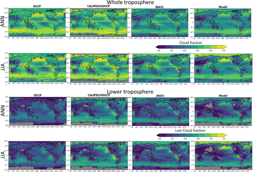
3814                                      P. T. M. Ha et al.: Effects of heterogeneous reactions on tropospheric chemistry

and Wang, 2020). Indeed, the O3 responses are controlled by      proximate 10 % reduction of O3 in both seasons (Li et al.,
several mechanisms, including heterogeneous effects of HO2       2018).
and N2 O5 onto aerosols (Kanaya et al., 2009; Li et al., 2019;      Another vital process taking place on particles is the HRs
Liu and Wang, 2020; Taketani et al., 2012).                      of peroxy radicals (HO2 and RO2 ). Peroxy radicals are the
   Stationary observations and laboratory experiments are        primary chain carriers driving O3 production in the tropo-
important for enhancing the understanding of the tropo-          sphere. Moreover, it can drive the hydrocarbon and NOx con-
spheric chemistry of O3 and other essential components           centrations, which are important for nocturnal radical chem-
(NOx , HOx ). However, direct observation of vertical O3 dis-    istry (Geyer et al., 2003; Richard, 2000; Salisbury et al.,
tribution, including upper tropospheric O3 , was not available   2001). In the past, the HR(HO2 ) effects have been well con-
before 1970. It has been deployed only at limited sites across   sidered in the laboratory (Macintyre and Evans, 2011) and
the globe. Global atmospheric modeling is a useful method        field observations (Kanaya et al., 2001, 2002a, b, 2003, 2007;
to reanalyze or forecast the past and future changes in O3 and   Taketani et al., 2012), but many technical problems (e.g., de-
their effects on human health and the climate. To serve this     tecting HO2 ) have created difficulties that challenge its re-
task, atmospheric models use both laboratory and observa-        ported importance in the troposphere, as asserted from re-
tional data to help achieve accurate simulations of O3 and its   cent studies (Liao and Seinfeld, 2005; Martin et al., 2003;
precursors (HOx , NOx , hydrocarbons). To date, many mod-        Tie et al., 2001). More recently, global modeling reports
eling studies have suggested that heterogeneous chemistry be     have described that the inclusion of HO2 uptake can affect
included in a standard model for tropospheric chemistry (Ja-     atmospheric constituents strongly by the increment in tro-
cob, 2000; Macintyre and Evans, 2010, 2011; de Reus et al.,      pospheric abundances for carbon monoxide (CO) and other
2005).                                                           trace gases because of reduced oxidation capacity (Lin et al.,
   One fundamentally important HR in the troposphere is          2012; Macintyre and Evans, 2011). The HOx loss on aerosols
the uptake of N2 O5 onto aqueous aerosols, known as a re-        can reduce O3 concentrations by up to 33 % in remote areas
moval pathway for NOx at night (Platt et al., 1984). Actu-       and up to 10 % in a smog episode (Saathoff et al., 2001; Take-
ally, NOx plays crucially important roles in the troposphere     tani et al., 2012). The HOx loss on sea salt, sulfate, and or-
because it controls the cycle of HOx and the production rate     ganic carbon in various environments can decrease HO2 lev-
of tropospheric O3 (Logan et al., 1981; Riemer et al., 2003).    els by 6 %–13 %, 10 %–40 %, and 40 %–70 %, respectively
The morning photochemistry can be affected by NO3 and            (Martin et al., 2003; Taketani et al., 2008, 2009; Tie et al.,
N2 O5 , which are important nocturnal oxidants. Since the        2001). For RO2 with a typical representative of CH3 CO.O2
early 1980s, the role of urban NOx chemistry in Los An-          (peroxyacetyl radical, PA), it plays a big role in the long-
geles pollution (National Research Council, 1991) has been       range transport of pollution (VOC, NOx ) (Richard, 2000;
acknowledged, but the proclamation of nighttime radicals re-     Villalta et al., 1996). It can bring NOx from polluted domains
mained sparse. It was only recognized in the past decade         as peroxyacyl nitrates (PAN) to remote regions in the ocean
that N2 O5 radical chemistry could have a much more per-         and higher altitudes (Qin et al., 2018; Richard, 2000). The
ceptible effect stemming from reasons including a refined        concentrations of HO2 and RO2 at nighttime in the marine
understanding of heterogeneous processes occurring at night      boundary layer were measured and confirmed (Geyer et al.,
(Brown and Stutz, 2012). The HR of N2 O5 was revealed un-        2003; Salisbury et al., 2001). Moreover, some evidence sug-
der different meteorological conditions in the US, Europe,       gests uptake of HO2 and PA on clouds, aqueous aerosols,
and China (photosmog, high relative humidity (RH), or sea-       and other surfaces in high-humidity conditions, although the
sonal variation) for particles of various types: ice, aqueous    mechanism is uncertain (Geyer et al., 2003; Jacob, 2000;
aerosols with organic-coating, urban aerosols, dust, and soot    Kanaya et al., 2002b; Liao and Seinfeld, 2005; Lin et al.,
(Apodaca et al., 2008; Lowe et al., 2015; Qu et al., 2019;       2012; Richard, 2000; Salisbury et al., 2001). The predomi-
Riemer et al., 2003, 2009; Wang et al., 2018, 2017; Xia et       nance of peroxy uptake to clouds results from the ubiquitous
al., 2019). The uptake of N2 O5 can markedly enhance ni-         existence and larger SAD maxima of cloud droplets in the at-
trate concentration in nocturnal chemistry or PM2.5 explo-       mosphere. Indeed, aqueous-phase chemistry might represent
sive growth events in summer, decrease NOx , and either in-      an important sink for O3 (Lelieveld and Crutzen, 1990). In
crease or decrease O3 concentrations in different NOx condi-     addition, PA loss on aqueous particles can mediate the loss
tions (Dentener and Crutzen, 1993; Qu et al., 2019; Riemer et    of PAN (CH3 CO.O2 NO) in fog (Villalta et al., 1996). Some
al., 2003; Wang et al., 2017). Even during daytime, N2 O5 in     modeling studies indicate that HOx loss (including HO2 loss)
the marine boundary layers can enhance the NOx to HNO3           on aqueous aerosols reduces OH by 2 % , increases CO by
conversion, and chemical destruction of O3 (Osthoff et al.,      7 % and increases O3 by 0.5 % in the annual mean global
2006). A 10–20 ppbv reduction of O3 because of N2 O5 up-         burden (Huijnen et al., 2014). However, in a coastal environ-
take in the polluted regions of China has also been reported     ment in the Northern Hemisphere it increases OH by 15 %
(Li et al., 2018). At mid- to high latitudes, N2 O5 uptakes on   and reduces HO2 by 30 % (Sommariva et al., 2006; Thorn-
sulfate aerosols could engender 80 % and 10 % NOx reduc-         ton et al., 2008).
tion, respectively, in winter and summer, leading to an ap-

Geosci. Model Dev., 14, 3813–3841, 2021                                          https://doi.org/10.5194/gmd-14-3813-2021
P. T. M. Ha et al.: Effects of heterogeneous reactions on tropospheric chemistry                                              3815

   Although the contributions of each uptake category to tro-      erogeneous reactions on PSC surfaces. In the framework
pospheric chemistry differ and must be considered both sep-        of MIROC-Chem, CHASER is coupled with the MIROC-
arately and as a whole, few studies have provided a global         AGCM atmospheric general circulation model (version 4;
overview of heterogeneous chemistry the comprehensively            Watanabe et al., 2011). The meteorological fields simulated
examines the uptakes of N2 O5 , HO2 , and RO2 on widely            by MIROC-AGCM were nudged toward the 6-hourly NCEP
various particles. For instance, uptakes of both N2 O5 and         FNL data (https://rda.ucar.edu/datasets/ds083.2/, last access:
HO2 tend to reduce O3 in particular environments (Li et al.,       30 October 2018). For this study, the spatial resolution of
2018; Saathoff et al., 2001; Taketani et al., 2012), but the       the model was set as T42 (about 2.8◦ × 2.8◦ grid spacing)
HO2 loss on clouds can increase the tropospheric O3 bur-           in horizontal and L36 (surface to approx. 50 km) in vertical.
den (Huijnen et al., 2014). The latter trend is not widely         Anthropogenic emissions for O3 and aerosol precursors like
suggested yet because the cloud chemistry is still neglected       NOx , CO, VOCs, and SO2 are specified using the HTAP-
in many O3 models (Stadtler et al., 2018; Thornton et al.,         II inventory (Janssens-Maenhout et al., 2015), with biomass
2008). The predominant effects of HO2 uptake on aerosols           burning emissions derived from the MACC reanalysis sys-
compared to the effect by N2 O5 were reported during the           tem (Inness et al., 2013).
summer smog condition (Saathoff et al., 2001) but with lack           In the model, the aerosol concentrations for black carbon
of confirmation on a global scale. Moreover, the heteroge-         (BC) / organic carbon (OC), sea salt, and soil dust are han-
neous effects of RO2 have been investigated only insuffi-          dled by the SPRINTAR module, which is also based on the
ciently (Jacob, 2000). In this study, we examine these un-         CCSR/NIES AGCM (Takemura et al., 2000). The bulk ther-
certainties using the global model CHASER to perceive the          modynamics for aerosols are applied, including SO2− 4 chem-
respective and total effects of the HRs of N2 O5 , HO2 , and       istry (SO2 oxidation with OH, O3 /H2 O2 , which is cloud-pH
RO2 on the tropospheric chemistry. For the interface of HRs        dependent) SO2−        −     +         2−
                                                                                   4 –NO3 –NH4 and SO4 –dust interaction.
in the atmosphere, we tentatively consider surfaces of cloud
particles and those of aerosols and discuss details of its ef-
                                                                   2.2   Heterogeneous reactions in the chemistry–climate
fects in this study. In the following text, the research method,
                                                                         model (CHASER)
including model description and configuration, is described
in Sect. 2. In Sect. 3.1, our model is verified with available
observations including ground stations and ship, aircraft, and     The CHASER-V4 model considers HRs in both the tropo-
satellite measurements, particularly addressing the roles of       sphere and stratosphere. In this work, we particularly ex-
the HRs. The global effects of N2 O5 , HO2 , and RO2 up-           amine HRs in the troposphere. In the current version of
take are discussed in Sect. 3.2 to elucidate cloud particles       CHASER, tropospheric HRs are considered for N2 O5 , HO2 ,
and aerosol effects. Section 3.3 will discuss sensitivities of     and RO2 , using uptake coefficients for the distinct surfaces
tropospheric chemistry to the magnitudes of HRs. Section 4         of aerosols (sulfate, sea salt, dust, and organic carbons) and
presents a summary and concluding remarks.                         cloud particles (liquid/ice) as listed in Table 2. Although
                                                                   some other views incorporate the catalysis of transition metal
                                                                   ions (TMIs) Cu(I)/Cu(II) and Fe(II)/Fe(III) for the HO2 con-
2     Method                                                       version on aqueous aerosols (Li et al., 2018; Mao et al., 2013;
                                                                   Taketani et al., 2012), this mechanism remains uncertain (Ja-
2.1    Global chemistry model                                      cob, 2000). The TMI mechanism might lead to either H2 O2
                                                                   (Jacob, 2000) or H2 O products (Mao et al., 2013). How-
The global chemistry model used for this study is CHASER           ever, this may not cause any significant difference, since re-
(MIROC-ESM) (Sudo et al., 2002; Sudo and Akimoto, 2007;            cycling HO2 from H2 O2 is ineffective (Li et al., 2018). For
Watanabe et al., 2011), which considers detailed photochem-        this study, the uptake of HO2 is affirmed with H2 O2 as the
istry in the troposphere and stratosphere. The chemistry com-      product (Loukhovitskaya et al., 2009; Taketani et al., 2009),
ponent of the model, based on CHASER-V4.0, calculates              as it is generally used in many atmospheric models such that
the concentrations of 92 chemical species and 262 chemi-           this is not counted as a terminal sink for HO2 (Jacob, 2000;
cal reactions (58 photolytic, 183 kinetic, and 21 heteroge-        Lelieveld and Crutzen, 1990; Morita et al., 2004; Thornton et
neous reactions including reactions on polar stratospheric         al., 2008). The RO2 uptakes are assumed with inert products,
clouds); more details on CHASER can be found in an earlier         as suggested by Jacob (2000). The heterogeneous pseudo-
report of the literature (Morgenstern et al., 2017). Its tropo-    first-order loss rate β for the species i is given using the the-
spheric chemistry considers the fundamental chemical cycle         ory of Schwartz (Dentener and Crutzen, 1993; Jacob, 2000;
of Ox –NOx –HOx –CH4 –CO, along with oxidation of non-             Schwartz, 1986), in which it is simply treated with the mass
methane volatile organic compounds (NMVOCs). Its strato-           transfer limitations operating two conductances represent-
spheric chemistry simulates chlorine and bromine-containing        ing free molecular and continuum regimes for tropospheric
compounds, CFCs, HFCs, carbonyl sulfide (OCS), NO2 , and           clouds and aerosols, in addition to using reactive uptake co-
the formation of polar stratospheric clouds (PSCs) and het-        efficient (γ ) instead of the mass accommodation coefficient

https://doi.org/10.5194/gmd-14-3813-2021                                             Geosci. Model Dev., 14, 3813–3841, 2021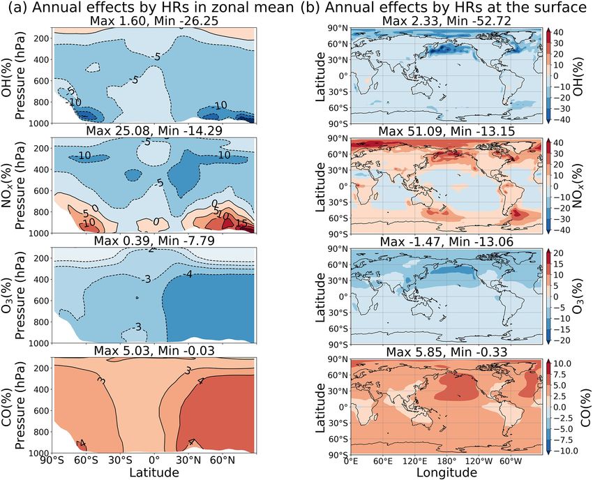
3816                                        P. T. M. Ha et al.: Effects of heterogeneous reactions on tropospheric chemistry

as follows:                                                        1993; Jacob, 2000). One study (Dentener and Crutzen, 1993)
                                                                   used a constant γN2 O5 of 0.1 for uptake on sea salt, sul-
      X 4         Rj −1

βi =             +       Aj ,                               (1)    fate, and cloud particles. They also revealed that a smaller
       j
           νi γij Dij                                              γN2 O5 of 0.01, which had been reported as laboratory mea-
                                                                   surements, is insensitive to effects on tropospheric oxidant
where νi stands for the mean molecular speed (cm s−1 ) of          components. Results of another study (Jacob, 2000) indi-
species i, Dij is the gaseous mass transfer (diffusion) coef-      cated constants γN2 O5 = 0.1 and γHO2 = 0.2 for uptakes on
ficient (cm2 s−1 ) of species i for particle type j , and Aj ex-   both liquid clouds and aerosols, the latter aiming to involve
presses the surface area density (cm2 cm−3 ) for particle type     HO2 scavenging by clouds without accounting for details of
j . In the model, the particle size and effective radius Rj for    aqueous-phase chemistry. For ice crystals, Jacob (2000) sug-
aerosols are calculated as a function of RH (Takemura et al.,      gested γHO2 = 0.025 based on a report by Cooper and Ab-
2000). The aerosol concentrations are based on SPRINTAR            batt (1996). Jacob (2000) recommended using γRO2 = 0.1 for
for BC/OC, sea salt, and dust (Takemura et al., 2000). The         hydroxy-RO2 group produced by oxidation of unsaturated
surface area density (SAD) for aerosols (Aj ) is estimated us-     hydrocarbons and γRO2 = 4 × 10⁻³ for PA. The γ values for
ing lognormal distributions of particle size (SFj ) with mode      aerosols are assumed to be fundamentally the same as those
radii variable with the RH (Sudo et al., 2002) as follows          for liquid cloud particles in this study. It is noteworthy that
                                                                   the γ values for cloud particles are given tentatively in this
Aj,ae = CN · 4π Rj2 · SFj ,                                 (2)    study and are adjusted based on evaluation of the resulting
                                                                   species concentrations of O3 , NOy , and OH with the obser-
where CN represents number density (cm−3 ) and Rj signi-           vations.
fies the effective radii (cm) of particle type j . To calculate
SAD for cloud particles, the liquid water content (LWC) and
ice water content (IWC) in the AGCM are converted using            2.3   Experiment setup
the cloud droplet distribution of Battan and Reitan (1957)
and the relation between IWC and the surface area density          In this study, simulations of two types were conducted to
for ice clouds (Lawrence and Crutzen, 1998; McFarquhar             isolate the distinct effects of each HR for the surface types
and Heymsfield, 1996).                                             considered in the model (Tables 3 and S1). Whereas a con-
                                                                   trol simulation standard (STD) run considers all HRs, cases
Ac = 10−4 · IWC0.9                                                 with no HRs (noHR) cases intentionally ignore one or all of
    Aj,ice = 3 · Ac ,                                       (3)    the HRs to calculate effects of individual HRs. The sensi-
                                                                   tivity runs turned off the separate HRs onto clouds (liquid
In these equations, Ac represents the cross-section area for       and ice), and aerosols were also added to exploit the sepa-
ice crystals (cm2 cm−3 ). For liquid clouds, the following         rate aerosol-heterogeneous and cloud-heterogeneous effects,
holds:                                                             as suggested in many earlier studies (Apodaca et al., 2008;
                                                                   Jacob, 2000; Lelieveld and Crutzen, 1990, 1991; Morita et
                         3
Aj,liq = LWC × 10−6 ·       .                               (4)    al., 2004). All simulations were run in the 2009–2017 time-
                         Rj                                        frame, with 2009 being treated as a spin-up year. The HR ef-
The uptake coefficient parameter (γ ) is defined as the net        fects are determined as the differences between noHR cases
probability that a molecule X undergoing a gas-kinetic col-        and an STD simulation as in Eq. (5):
lision with a surface is actually taken up onto the surface.
Although several recent model studies that consider depen-                        (STDi − noHR(j )i )
dency of γ on RH and/or T, the majority of the earlier stud-       Impact(i)j =                       · 100 (%),              (5)
                                                                                      noHR(j )i
ies use constant γ values that only vary with aerosol parti-
cle compositions (Chen et al., 2018; Evans and Jacob, 2005;
Macintyre and Evans, 2010, 2011). For one study, γHO2 for          where STDi stands for the concentration of investigated at-
the uptake onto aqueous aerosols is considered with pH de-         mospheric component i in the STD run and noHR(j )i de-
pendence (Thornton et al., 2008). However, another study           notes the concentration of component i in the sensitivity run
demonstrated that the uptake is large, irrespective of the sol-    in which the HRs of/onto j was ignored (j could be N2 O5 ,
ubility in cloud water or pH (Morita et al., 2004). There-         HO2 , RO2 , clouds, aerosols).
fore, we instead choose γHO2 as fixed values depending on             An additional sensitivity test was run to examine the sensi-
the type of particle. Indeed, from Eq. (1) it is apparent that     tivity of the troposphere’s responses with the amplified HRs
uptake coefficients should be unimportant for uptake onto          magnitudes (Table S1). These simulations only apply for
large particles such as cloud droplets. In this study, γ for       HR(N2 O5 ) and HR(HO2 ) to verify some uncertainties that
cloud particles of liquid and ice phases are given based           have been argued among earlier studies (Chen et al., 2018;
on suggestions from earlier reports (Dentener and Crutzen,         Evans and Jacob, 2005; Macintyre and Evans, 2010, 2011).

Geosci. Model Dev., 14, 3813–3841, 2021                                            https://doi.org/10.5194/gmd-14-3813-2021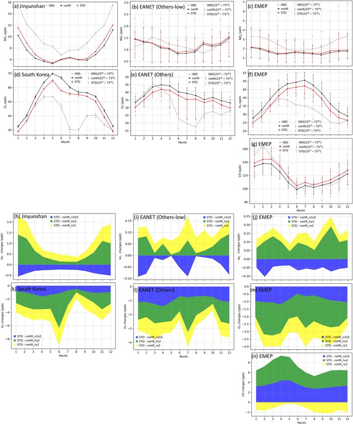
P. T. M. Ha et al.: Effects of heterogeneous reactions on tropospheric chemistry                                                                3817

Table 1. Computation packages in the chemistry–climate model CHASER.

               Base model                                   MIROC4.5 AGCM
               Spatial resolution                           Horizontal, T42 (2.8◦ × 2.8◦ ); vertical, 36 layers (surfaces ap-
                                                            prox. 50 km)
               Meteorology (u, v, T )                       Nudged to the NCEP2 FNL reanalysis
               Emission (anthropogenic, natural)            Industry traffic, vegetation, ocean,
                                                            Biomass burning specified by MACC reanalysis
               Aerosol                                      BC/OC, sea-salt, and dust
                                                            BC aging with SOx /secondary organic aerosol (SOA) production
               Chemical process                             94 chemical species, 263 chemical reactions (gas phase, liquid phase,
                                                            non-uniform)
                                                            Ox –NOx –HOx –CH4 –CO chemistry with VOCs
                                                            SO2 , dimethyl sulfide (DMS) oxidation (sulfate aerosol simulation)
                                                            SO4 –NO3 –NH4 system and nitrate formation
                                                            Formation of SOA
                                                            BC aging
                                                            (+) Heterogeneous reactions: 8 reactions of N2 O5 , HO2 , RO2 ; constant
                                                            uptake coefficients (γ ) on types of aerosols (ice, liquid, sulfate, sea salt,
                                                            dust, OC)

Table 2. Heterogeneous reactions in CHASER.

                           No        Reactions                             γice        γliq      γsulf      γsalt      γdust        γoc
                           (R1)      HO2 → 0.5H2 O2 + 0.5O2                0.02        0.1         0.1        0.1        0.1        0.1
                           (R2)      N2 O5 → 2HNO3                         0.01       0.08         0.1        0.1        0.1        0.1
                           RO2 → products
                           (R3)      HOC2 H4 O2 → product                  0.02       0.2        0.2          0.2       0.2        0.2
                           (R4)      HOC3 H6 O2 → product                  0.02       0.2        0.2          0.2       0.2        0.2
                           (R5)      ISO2 → product                        0.01        0.1        0.1         0.1        0.1        0.1
                           (R6)      MACRO2 → product                      0.01        0.1        0.1         0.1        0.1        0.1
                           (R7)      CH3 COO2 → product                       0     0.001      0.004       0.004      0.004      0.004
                         References and the details of these adjustments are given in the main text. The RO2 uptakes are assumed with inert
                         products, as suggested by Jacob (2000). ISO2 is denoted for peroxy radicals from C5 H8 + OH, and MACRO2 stands
                         for peroxy radicals from methacrolein (CH2 = C(CH3 )CHO).

2.4   Observation data for model evaluation                                             Additionally, we exploited ship-based observational data
                                                                                     from R/V Mirai cruise (http://www.godac.jamstec.go.jp/
Model simulations with and without HRs are evaluated                                 darwin/e, last access: 30 June 2020) undertaken by the
distinctively with stationary, ship-based, aircraft-based, and                       Japan Agency for Marine-Earth Science and Technology
satellite-based measurements. The observational informa-                             (JAMSTEC). This study used data for surface CO and
tion, locations of the surface sites, and ship or aircraft tracks                    O3 concentrations in summer 2015–2017 along the Japan–
for the observations used for this study are summarized in                           Alaska and Japan–Indonesia–Australia routes (Kanaya et al.,
Table 4 and Fig. 1.                                                                  2019). The model data were compiled in hourly time steps
   EANET is well known as the Acid Deposition Monitor-                               and were interpolated corresponding with the Mirai time
ing Network in eastern Asia. The monthly data from 45 sta-                           step and coordinates. For verification of the vertical tropo-
tions over 13 countries during 2010–2016 were used to ver-                           spheric profiles, we used Atmospheric Tomography (ATom1)
ify surface concentrations of aerosols (sulfate, nitrate) and                        aircraft measurements (https://espo.nasa.gov/atom/content/
trace gases (HNO3 , NOx , O3 ) in eastern Asia. We also used                         ATom, last access: 30 June 2020) for NO2 , OH, CO, and O3 .
data of the European Monitoring and Evaluation Programme                                The simulated tropospheric ozone was also evalu-
(EMEP), which compiles observations over 245 European                                ated using the tropospheric column O3 (TCO) derived
stations.                                                                            from the OMI satellite data (https://daac.gsfc.nasa.gov/,

https://doi.org/10.5194/gmd-14-3813-2021                                                                      Geosci. Model Dev., 14, 3813–3841, 2021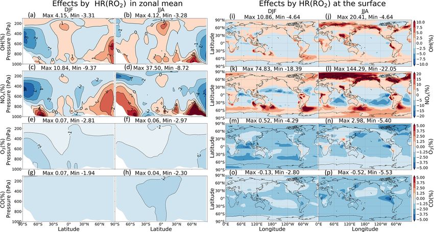
3818 P. T. M. Ha et al.: Effects of heterogeneous reactions on tropospheric chemistry
Table 3. Main sensitivity simulations for HRs in this work.
No. Simulation ID HR: N2 O5 HR: HO2 HR: RO2 HRs on clouds HRs on aerosols
1 STD × × ×
2 noHR
3 noHR_n2o5 × ×
4 noHR_ho2 × ×
5 noHR_ro2 × ×
6 noHR(Cld) ×
7 noHR(Ae) ×
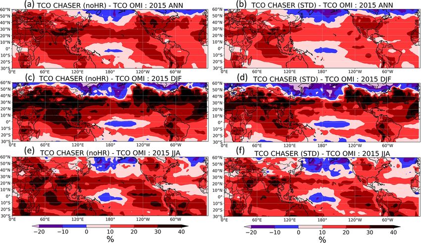
last access: 25 February 2020). For distribution of the ever, for the lower troposphere over the region, the cloud
cloud fraction, satellite data from International Satel- fraction calculated using CHASER in JJA appears to be over-
lite Cloud Climatology Project (ISCCP, https://isccp.giss. estimated (Fig. 2, the fourth row), suggesting that the result-
nasa.gov/, last access: 12 June 2020), GCM-Oriented ing HR effects would also be exaggerated to some extent.
CALIPSO Cloud Products (CALIPSO-GOCCP, https://
eosweb.larc.nasa.gov/project/calipso/calipso_table, last ac-
3.1.2 Verification with stationary observations
cess: 12 June 2020), and Japanese 55-year reanalysis (JRA-
55 – https://doi.org/10.5065/D6HH6H41, Japan Meteorolog-
ical Agency/Japan, 2013) were used. Verifications with EANET and EMEP stationary observa-
Model bias and normalized root-mean-squared error tions were conducted to assess the model performance on
(NRMSE) for each species were calculated as shown be- land domains of eastern Asia and Europe, particularly ad-
low, where n is the number of available data (number of sta- dressing the roles of the heterogeneous reactions considered
tions × time step). for this study.
The mass concentrations of particulate matter (PM2.5 );
n
P
Model − observation sulfate (SO2− −
4 ); nitrate (NO3 ); and gaseous HNO3 , NOx ,
1 O3 , and CO (CO only for EMEP) of 2010–2016 were eval-
bias = (6)
n uated (see Figs. S1 to S8 for monthly concentrations and
s
n Fig. S9 for correlations). In general, the model can mod-
(Model−observation)2
P
1 erately reproduce the PM2.5 , SO2− −
4 , and NO3 aerosol con-
n centrations at these locations (R = 0.3–0.7, Table 5), al-
NRMSE = (7)
Observation though PM2.5 was underestimated, sulfate was overestimated
slightly. Nitrate was underestimated for EANET and overes-
timated for EMEP. It is noteworthy that the model perfor-
mance for EMEP stations was better than that for EANET.
3 Results and discussion
The PM2.5 concentration was better estimated with the inclu-
3.1 Model verifications sion of N2 O5 and HO2 uptakes (bias reduction in Table 5).
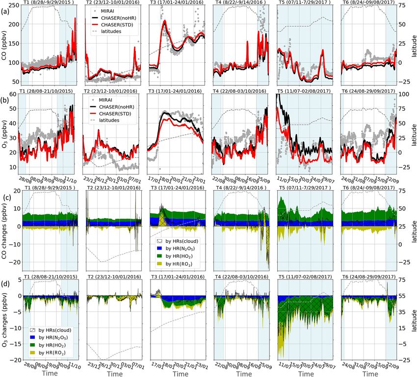
Figure 3a–g present the median values of NOx , O3 , and CO
3.1.1 Cloud verification for grouped stations in the Chinese and South Korean re-
gions (stations in China: Jinyunshan; stations in South Ko-
For this study, we tentatively consider HRs on the cloud par- rea: Kanghwa, Imsil, Cheju), remote stations with low NOx
ticle surface. Given the great uncertainties related to the re- levels of EANET, and all EMEP stations. Figure 3h–n show
action coefficient (γ ) (Macintyre and Evans, 2010, 2011), changes in NOx , O3 , and CO for these stations. The model’s
the cloud distributions must be examined adequately in the positive bias for NO− 3 at Kanghwa as a remote area is differ-
model to the greatest extent possible. The model-calculated ent from the model underestimates at other EANET stations
cloud distributions were verified using satellite observation (e.g., Bangkok, Hanoi, and Hongwen in Fig. S1). These high
data ISCCP D2, CALIPSO-GOCCP, and reanalysis data negative biases for NO− 3 can be associated with undervalu-
JRA55. ation for NOx and can thereby lessen the effects of N2 O5
For the entire troposphere, the calculated cloud fraction uptake.
was generally underestimated against the satellite observa- Nitric acid in both regions was overestimated. The cor-
tions and reanalysis data (Fig. 2, the first row). In the North relations, biases, and normalized root-mean-square error
Pacific region in JJA (Fig. 2, the second row), when the cloud (NRMSE) of the model for SO2− −
4 , NO3 , and HNO3 are in the
fraction peaked in the region, the model was able to repro- ranges reported in a multi-model study by Bian et al. (2017)
duce the satellite observations (ISCCP and CALIPSO). How- (Table 6).
Geosci. Model Dev., 14, 3813–3841, 2021 https://doi.org/10.5194/gmd-14-3813-2021
P. T. M. Ha et al.: Effects of heterogeneous reactions on tropospheric chemistry                                                3819

Figure 1. Locations of EANET stations (a), EMEP stations (b), Mirai cruises (c), and ATom1 flights (d). The source for panel (a) is
https://monitoring.eanet.asia/document/overview.pdf (last access: 12 June 2020).

Table 4. Datasets used for verification in this study.

      Verified species                      Regions                    Data            Time series          Time step
      Sulfate, nitrate, NOx , O3 , HNO3     Eastern Asia               EANET           2010–2016            Daily to 2-weekly
      Sulfate, nitrate, NOx , O3 , CO       Europe                     EMEP            2010–2016            Hourly
      CO, O3                                Surface of the Pacific     Mirai           Aug, Sep 2015        30 min
                                            Ocean      (Australia–
                                            Indonesia–Japan–
                                            Alaska)
                                                                                       Jan, Aug, Sep 2016
                                                                                       Jul, Aug, Sep 2017
      NO2 , OH, CO, O3                      Various altitudes above    ATom1           Aug 2016             30 min
                                            the Pacific and Atlantic
                                            oceans
      TCO                                   60◦ S–60◦ N (satellite)    OMI             2010–2016            Daily
      Cloud fraction                        Global (satellite)         ISCCP           2000–2009            Monthly
                                            Global (satellite)         CALIPSO-GOCCP   2007–2017            Monthly
                                            Global (reanalysis)        JRA55           2000–2015            6-hourly

https://doi.org/10.5194/gmd-14-3813-2021                                               Geosci. Model Dev., 14, 3813–3841, 2021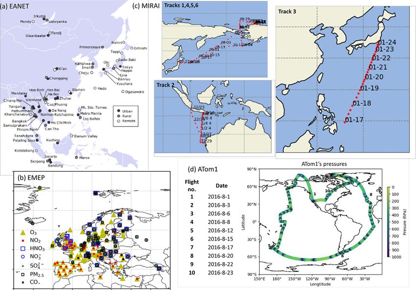
3820                                         P. T. M. Ha et al.: Effects of heterogeneous reactions on tropospheric chemistry

Figure 2. Comparisons for cloud fraction in the whole troposphere (first and second rows) and lower troposphere (third and fourth rows).
ANN denotes annual mean, and JJA denotes June + July + August mean. The first column is for ISCCP (2000–2009), the second column is
for CALIPSO/GOCCP (2007–2017), and third and fourth columns are for JRA55 and CHASER (2000–2015), respectively. Color bars are
the same for all panels. In ISCCP and CALIPSO data, the pressure boundary layer of the low troposphere is > 680 hPa. In JRA55, the low
troposphere was defined as 850–1100 hPa of pressure.

   The NOx concentration for eastern Asia and Europe was              face NOx as previously investigated by Sekiya et al. (2018).
underestimated, with significant bias for polluted Asian loca-        Moreover, the low reproducibility of the model for NOx is
tions (Bangkok, Metro Manila, Nai Muaeng, Samutprakarn,               probably caused by lacking mechanisms that reduce HNO3
Si Phum, Ulaanbaatar, not shown). In Fig. 3a and c, sim-              and enhance NOx in our model. One possible mechanism is
ulated NOx levels still underestimated the observed values            the heterogeneous reaction of HNO3 on soot surfaces (Re-
for Chinese and European regions, at which the observed               action R8) (Akimoto et al., 2019, and references therein):
NOx could reach 16 and 7 ppb, respectively. For the low-              HNO3 + soot → NO + NO2 (Reaction R8).
NOx EANET region, excluding the abovementioned sites                     The additional Reaction (R4) followed by NO2 uptakes
(Fig. 3b), simulated NOx levels turned to overestimate the            onto soot (Jacob, 2000), NO2 + particles → 0.5 HONO + 0.5
observed levels in January, February, September, and Octo-            HNO3 (Reaction R9), can be expected to increase NO and
ber. The increasing effects of NOx attributable to heteroge-          decrease O3 via the consequent titration reaction. These
neous reactions, although minor, mitigated these underesti-           changes could reduce the model overestimates for HNO3 and
mations (Fig. 3a–c). Although NOx was partly reduced via              O3 and the model underestimates for NOx with EANET and
uptake of N2 O5 , the NOx level was mostly increased because          EMEP stations. Further tests for this issue shall be discussed
of HO2 and RO2 uptakes (Fig. 3h–j).                                   in a future report.
   In this comparison, the low correlations of the model with            CO for EMEP was partly underestimated by the model,
EANET and EMEP sites for HNO3 and NOx are still a prob-               especially during January–March (Fig. 3g). This underesti-
lem. The high biases for nitrogen species could be ascribed           mate was mitigated by increasing effects because of HRs of
to the low horizontal resolution in this study (∼ 2.8◦ ). Higher      N2 O5 and HO2 . The uptakes of RO2 , in contrast, minorly
resolutions could improve the model reproduction for sur-             reduced CO levels (Fig. 3n) so that the model bias was wors-

Geosci. Model Dev., 14, 3813–3841, 2021                                                 https://doi.org/10.5194/gmd-14-3813-2021
P. T. M. Ha et al.: Effects of heterogeneous reactions on tropospheric chemistry 3821
ened slightly. For O3 , whereas the model tends to overesti-
Table 5. Model correlations and biases with EANET/EMEP observations: three-sigma-rule outlier detection is applied for each station before calculating all data. For NOx , all data
were filtered once more using the two-sigma-rule. Bias of the sensitivity run is shown in bold if it is higher than the bias of the STD run. R has no unit; the units in brackets are for
mate this tracer for both regions (Fig. 3d–f), O3 reduction
effects of all HRs (Fig. 3k–m) alleviated the model overesti-
mates from April to December, although advanced reduction
is still needed. In January–March, the model tended to un-
CO
[ppb]
0.534
−3.439
− 9.062
− 6.822
− 6.896
−2.276
derestimate O3 levels (Fig. 3d–f), which was exaggerated by
reduction effects for O3 . In general, the STD simulation with
coupled HRs partly improved the agreement related to the
particulate and gaseous species, showing less bias than that
[ppb]
0.651
4.071
7.189
5.013
5.489
4.893
O3
of simulations without HRs (Table 5).
[ppb]
0.698
−0.773
− 0.895
−0.707
− 0.895
− 0.833
NOx
3.1.3 Verification with ship-based measurements
The model simulations were also verified with O3 and CO
observations from the Research Vessel (R/V) Mirai for the
[ppb]
0.116
0.081
0.067
0.07
0.078
0.079
HNO3
Pacific Ocean region. This study specifically examines data
EMEP
from the four cruises of R/V Mirai for the Japan–Alaska re-
gion (40–75◦ N, 140◦ E–150◦ W) in summer, designated as
[µg m−3 ]
0.715
0.273
0.106
0.042
0.335
0.275
NO−
3
MR15-03 leg 1 and leg 2 (28 August–21 October 2015, la-
beled as Track 1 in this study), MR16-06 (22 August–3 Octo-
ber 2016 as Track 4), MR1704 leg 1 (11 July–2 August 2017
[µg m−3 ]
0.633
0.784
0.603
0.774
0.55
0.839
SO2−
as Track 5), and MR1705C (24 August–29 September 2017
4
as Track 6). Two other cruises during DJF for the Indonesia–
Australia region (5–25◦ S, 105–115◦ E) and Indonesia–Japan
region (10–35◦ N, 129–140◦ E) are also explored in this
[µg m−3 ]
0.475
−2.966
− 3.262
− 3.223
− 3.136
−2.858
PM2.5
study, respectively designated as MR15-05 leg 1 (23 Decem-
ber 2015–10 January 2016 as Track 2) and MR15-05 leg 2
(17–24 January 2016 as Track 3). All measuring data for CO
and O3 from the six cruises are respectively plotted in Fig. 4a
[ppb]
0.6
3.927
6.808
4.93
5.126
4.931
O3
and b as grey dots. The ship-based data used in this study was
partly reported (T1–4) in the work of Kanaya et al. (2019), in-
cluding the extraordinary peak of CO on 26 September 2016
[ppb]
0.233
−3.929
− 4.011
−3.869
− 4.02
− 4.008
NOx
exceeded 500 ppbv (off the scale in Fig. 4a-T4) associated
with heavy fires in Russia (Kanaya et al., 2019). Data for the
North Pacific region (40–60◦ N) are addressed in light-blue
[ppb]
0.177
0.311
0.292
0.295
0.312
0.305
HNO3
shades in Fig. 4 (T1, T4–6) for analysis in Sect. 3.2.
Table 7 shows correlation coefficients (plotted in
EANET
Fig. S10), indicating that the CHASER simulations for CO
[µg m−3 ]
0.379
−0.395
− 0.452
− 0.46
−0.37
− 0.427
NO−
3
and O3 are in good agreement with Mirai observations
(R = approx. 0.6). However, the model still shows some dis-
crepancies for both CO and O3 concentrations. In general,
the estimated CO and O3 are both reduced for T1 and T4–6 as
[µg m−3 ]
0.56
1.048
0.971
1.05
0.925
1.021
SO2−
4
compared to observations, whereas they are superior for the
data located in 20◦ S–20◦ N during T2–3. Overestimations
for CO and O3 occurring in the region with considerably low
levels of these species might be attributed to the lack of halo-
[µg m−3 ]
0.37
−7.526
−7.442
− 7.575
− 7.607
−7.38
PM2.5
gen chemistry in the model, as also discussed for the nearby
region in a past report (Kanaya et al., 2019). Underestimates
for O3 levels up to 70 ppbv in the higher latitudes (Fig. 4b:
Bias (noHR_n2o5)
T1, T4–6) are ascribable to the insufficient downward mixing
Bias (noHR_ho2)
Bias (noHR_ro2)
process of stratosphere O3 in the model (Kanaya et al., 2019).
Bias (noHR)
Except for the CO’s peak on 26 September 2016 mentioned
Bias (STD)
R (STD)
above, the mild reductions for CO (< 30 ppbv) in the model
during T1 and T4–6 as compared to the observations could
biases.
be attributed to the insufficient emission from territories, in-
https://doi.org/10.5194/gmd-14-3813-2021 Geosci. Model Dev., 14, 3813–3841, 2021
3822                                          P. T. M. Ha et al.: Effects of heterogeneous reactions on tropospheric chemistry

Figure 3. Monthly averaged concentrations at EANET and EMEP from 2010–2016 (a–g) and corresponding HR effects (h–n) for NOx : (a,
h) Jinyunshan (China), (b, i) other low-NOx EANET stations, and (c, j) EMEP stations; for O3 : (d, k) Korean stations, (e, l) other EANET
stations, and (f, m) EMEP stations; for CO: (g, n) EMEP stations. In (a)–(g), grey lines are observations (OBS), red lines are the STD
simulation, and black lines are the noHR simulation. All lines showed the median of monthly mean concentrations for each group of stations,
except (a). In (b)–(g), vertical thin lines with markers show the 25th–75th percentiles of monthly mean concentration at the particular group
of stations. In (h)–(n), blue fields are changes caused by HR(N2 O5 ), green fields are changes in HR(HO2 ), and yellow fields are changes
caused by HR(RO2 ).

Geosci. Model Dev., 14, 3813–3841, 2021                                                    https://doi.org/10.5194/gmd-14-3813-2021
P. T. M. Ha et al.: Effects of heterogeneous reactions on tropospheric chemistry                                                     3823

Table 6. Comparisons between EANET and EMEP observations with atmospheric models. Outlier detection follows that in Table 5. The
model result is shown in bold if it is better than or agreed with Bian’s report. R has no unit; units in brackets are for biases and NRMSE.

                    EANET                SO4 [µg m−3 ]             NO3 [µg m−3 ]               HNO3 [ppb]
                    This study           R = 0.56                  R = 0.379                   R = 0.177
                                         bias = 1.048              bias = − 0.395              bias = 0.311
                                         NRMSE = 0.954             NRMSE = 1.58                NRMSE = 2.491
                    Bian et al. (2017)   R = 0.449–0.640           R = 0.226–0.448             R = 0.098–0.370
                                         bias = 0.358–1.353        bias = 0.338–1.920          bias = 0.347–3.596
                                         NRMSE = 0.840–0.968       NRMSE = 1.494–2.080         NRMSE = 0.980–2.880
                    EMEP                 SO4 [µg m−3 ]             NO3 [µg m−3 ]               HNO3 [µg m−3 ]
                    This study           R = 0.633                 R = 0.715                   R = 0.116
                                         bias = 0.784              bias = 0.273                bias = 0.886
                                         NRMSE = 0.961             NRMSE = 0.91                NRMSE = 3.33
                    Bian et al. (2017)   R = 0.230–0.463           R = 0.393–0.585             R = 0.157–0.502
                                         bias = 0.452–1.699        bias = 0.539–1.421          bias = 0.570–3.836
                                         NRMSE = 0.514–0.818       NRMSE = 0.745–1.031         NRMSE = 0.908–2.542

ternational shipping, and aviation, as we used the HTAP-II              ing 50 000 µm2 cm−3 during JJA) and sulfate aerosols (ap-
emission inventory. These reductions for CO in Kanaya’s                 proximately 75 µm2 cm−3 in JJA). The model improvements
work are minor, e.g., for T1 (MR15-03 leg 1 and 2 in their              in reproducing CO by adding N2 O5 and HO2 uptake indi-
work), due to reanalysis data with finer horizontal resolution          cate that the appropriate mechanisms of these processes onto
(1.1◦ ) utilized for the CO emission rate (Kanaya et al., 2019).        cloud droplets and sulfate aerosols are well established in the
   The negative biases in the noHR simulations for CO are               model. For HR(RO2 ), which induces the smallest and oppo-
lower in the STD run for all cruises, as they are for the               site effects on CO compared with the effects of N2 O5 and
North Pacific region (second versus third/fourth/fifth data             HO2 uptakes, it can be stated in general for the total HR
rows for CO, Table 7). The CO-increasing effects by N2 O5               effects that including all three HRs partially improves the
and HO2 uptakes (Fig. 4c) are consistent with the comparison            model during Mirai cruises.
for EMEP. This is also true for CO-reduction effects because
of HR(RO2 ). Whereas the effects by N2 O5 and HO2 reduce                3.1.4   Verification using aircraft measurements
the model bias, the CO-reducing effects by HR(RO2 ) exag-
gerated the CO bias (second versus sixth data rows for CO               To verify the model performance in the free troposphere, we
in Table 7), which is already apparent for comparison with              used ATom1 aircraft measurements in August 2016 (for NO2 ,
EMEP (last column, Table 5).                                            OH, CO, and O3 ). Table 8 lists the model’s correlation co-
   For O3 level, the model underestimates (Table 7) are in              efficients and biases of each sensitivity run against ATom1.
the opposite direction to the O3 overestimates for EANET                Figure 5 shows observed and simulated concentrations of CO
and EMEP stations (Table 5). The lower panels presented                 and O3 during flight no. 2 in the North Pacific (NP) region.
in Fig. 4b show marked O3 reduction with all HRs (gaps                  Figure 6 exhibits vertical biases of the model and computed
between red and black lines), mostly contributed from the               HR effects caused by each HR for all ATom1 flights and NP
HO2 uptake onto cloud particles (Fig. 4d: green and hatched             region. The spatial and temporal concentrations are available
fields). This marked reduction of the O3 level is evident               in Fig. S11. Correlations are shown in Fig. S12.
at some points during the cruises, especially in the North                 In general, the model simulations for NO2 , OH, CO, and
Pacific region (the shaded areas) and for T5. Unlike com-               O3 adequately agree with aircraft measurements with R >
parisons for land domain data (Table 5), O3 reduction be-               0.5 (Fig. S12). However, NO2 and CO still tend to be un-
cause of HRs worsens the model underestimates during the                derestimated by the model, which is consistent with compar-
Mirai cruises. It is noteworthy that one cannot necessarily             isons for EANET/EMEP and Mirai observations. In Fig. 5,
confirm whether the STD run simulates these species bet-                the CO-increasing effects, mostly due to the uptake of N2 O5
ter than the noHR does because tropospheric CO and O3                   and HO2 (Fig. 6o), mitigated the negative bias of the model.
levels are controlled by a complicated chemical mechanism               This CO bias reduction was visible for all flight altitudes,
and an interplay of emission, transport, deposition, and lo-            the lower troposphere, and the North Pacific region (Table 8;
cal mixing in the boundary layers. As discussed later in                Fig. 6d and h). Both N2 O5 and HO2 uptakes show improve-
Sect. 3.2, the surface aerosols concentration in the western            ments for CO reproduction of the model. However, RO2 up-
Pacific Ocean is mostly dominated by liquid clouds (exceed-             take seems to worsen the model’s CO bias due to its reducing

https://doi.org/10.5194/gmd-14-3813-2021                                                   Geosci. Model Dev., 14, 3813–3841, 2021
3824 P. T. M. Ha et al.: Effects of heterogeneous reactions on tropospheric chemistry
Table 7. Model correlations and biases for Mirai. No outlier filtration is applied. The bias of the sensitivity run is shown in bold if it is higher
than the bias of STD run. R has no unit; the units in brackets are for biases.
CO [ppbv] O3 [ppbv] CO (40–60◦ N) [ppbv] O3 (40–60◦ N) [ppbv]
R (STD) 0.689 0.617 0.58 0.665
Bias (STD) −4.988 −4.996 −11.668 −3.493
Bias (noHR) − 10.324 −2.388 − 17.625 1.211
Bias (noHR_n2o5) − 8.127 −4.362 − 14.804 −2.738
Bias (noHR_ho2) − 9.036 −3.358 − 16.358 −0.226
Bias (noHR_ro2) −3.433 −4.431 −10.035 −2.526
Bias (noHR(cld)) − 6.821 −3.199 − 14.005 0.025
effect for CO (Fig. 6o and s), which is consistent with the Mi- is apparently extended in this region. However, the inclusion
rai comparison. of HR(HO2 ) leading to O3 increment (Fig. 6f) reduces O3
For the O3 level, the model generally overestimates O3 bias in this region, which might indicate that the O3 increase
when calculating for all altitudes or lower troposphere, which effect by HR(HO2 ) is verified, particularly in 500–900 hPa
is similar to the EANET/EMEP observations. In the North layers during ATom1.
Pacific region with P > 600 hPa (40–60◦ N, 198–210◦ W), We also verify the total uptake of N2 O5 , HO2 , and RO2
the model bias for O3 in STD run turns to underestimate (sec- onto ice and liquid clouds using data obtained from ATom1
ond data row and second column from the right, Table 8), flights within the free troposphere. As Table 8 shows, the
which might be similar with Mirai data verification for the inclusion of HRs onto clouds reduces the model biases for
western North Pacific (143◦ E–193◦ W). However, the under- CO and O3 in all calculations. In Fig. 6l–s, because the
layers (> 700 hPa) again show overestimation (second data HRs(cloud) effects occupy the major part of total HRs ef-
row – last column, Table 8). As Mirai and ATom1 data show, fects for NO2 , O3 , and OH, especially for NP region and
the underestimates for O3 exist at the marine boundary layer low troposphere (> 800 hPa), cloud uptakes could also con-
in the western North Pacific and extend to the upper tropo- tribute to the overall reduction in model bias against ATom1.
sphere (< 700 hPa) of the east side, which might be ascribed For O3 , HRs(cloud) mostly induce negative effects (Fig. 6m
to the insufficient downward mixing process of stratosphere and q). At the layer of 600–800 hPa in the NP region, this
O3 in the model as discussed previously. O3 reduction due to HR(RO2 ) onto clouds (Fig. 6q: yellow
The HR effects on O3 are generally negative effects and hatched patterns) might account for the model worsen-
(Fig. 6m), although they are small and barely recognizable in ing in O3 levels as described above. This result might prove
Fig. 5, which mitigates the model bias in the noHR run. This that cloud overestimation for the North Pacific, as revealed
model improvement is consistent for all flight altitudes, the at the beginning of this section, affects the model bias in this
low troposphere, and the North Pacific region (second versus region.
third data rows in Table 8). Both HR(N2 O5 ) and HR(RO2 )
typically contribute to this improvement (Fig. 6m and q). In 3.1.5 Verification with OMI satellite observation for
contrast, HR(HO2 ) seems to only reduce the model bias in a TCO
thin layer: from the ground up to 800 hPa for all flights and
700 hPa for the North Pacific region (Fig. 6m and q). At the We also tested STD and noHR simulations using the tropo-
bottommost layers in this region, the model’s overestimates spheric column ozone (TCO) derived from the OMI satellite
for O3 are reduced by the negative effects of HO2 uptake instrument (Figs. S13 and 7). In a large area of the North-
(Fig. 6f and q). The extension of model bias because of HO2 ern Hemisphere, the inclusion of HRs (STD run) generally
uptake above 800 hPa is attributable to its increasing effect on improved the consistency with the OMI TCO, as seen in
O3 level (Fig. 6m). We recognize that this O3 increase effect Fig. 7b, d, f with less overestimation than Fig. 7a, c, e, partic-
above 800 hPa is opposite to the effects for EANET/EMEP ularly enhancing the winter minima (first and second panels
and Mirai comparisons, which is discussed in Sect. 3.2 for in Fig. S13). This improvement in DJF is attributed mostly
HO2 uptake effects. to the reductive effects of HR(N2 O5 ) and HR(RO2 ) in the
The vertical means of model biases and changes for all lower (800 hPa) and middle troposphere (500 hPa), respec-
four species (NO2 , OH, CO, O3 ) are presented in Fig. 6. tively (see Fig. 10 for vertical profiles of HR(N2 O5 ) on O3
In general, the STD run reduces model biases for all four and Fig. 13 for vertical profiles of HR(RO2 )). In the North
species, with better performance for broader regions (all Pacific, HRs appeared to exaggerate O3 underestimates, es-
flights) than for the smaller region (North Pacific). In the pecially for latitudes higher than 40◦ N (Fig. 7) during the
North Pacific region, the negative bias for O3 is observed first half of the year (third panel, Fig. S13). However, such a
only for the 500–900 hPa layers (Fig. 6f). The model bias discrepancy, which was also observed from comparison for
Geosci. Model Dev., 14, 3813–3841, 2021 https://doi.org/10.5194/gmd-14-3813-2021P. T. M. Ha et al.: Effects of heterogeneous reactions on tropospheric chemistry 3825
Figure 4. Observed and simulated concentrations for CO (a) and O3 (b) and their changes caused by each HR (c, d) during Mirai cruises.
The left axis shows concentrations. Dashed lines show latitudes of cruises scaled with the right axis. The horizontal axis shows cruise travel
times. Light-blue areas show data in the North Pacific region (140–240◦ E, 40–60◦ N). In (a) and (b), grey dots are for observations, red lines
are for STD simulations, and black lines are for noHR simulations. In (c) and (d), blue fields are for changes in HR(N2 O5 ), green fields for
changes in HR(HO2 ), yellow fields for changes in HR(RO2 ), and hatched fields for changes in HRs (cloud). Note that in (d) all three fields
are stacked but in (c) only blue and green fields are stacked for better illustration of negative and positive changes.
R/V Mirai observations (Fig. 4), might result from other fac- simulations described in Table 3, additional runs that sepa-
tors such as deposition or vertical mixing rather than by HRs. rately turned off the uptakes onto clouds or aerosols for each
HR are also conducted to exploit the contributions of effects
3.2 HR effects to the troposphere.
This section presents a discussion of the global effects of 3.2.1 Distribution of clouds and aerosols surface area
HRs calculated using CHASER with their spatial distribu- density (SAD)
tions in the troposphere using standard (STD) and sensitivity
simulations (noHR_n2o5, noHR_ho2, noHRs_ro2, noHR) To obtain the parameters for uptake to clouds and aerosols,
for the meteorological year of 2011. Aside from the main SAD estimations are used together with cloud fraction and
https://doi.org/10.5194/gmd-14-3813-2021 Geosci. Model Dev., 14, 3813–3841, 20213826 P. T. M. Ha et al.: Effects of heterogeneous reactions on tropospheric chemistry
Table 8. Model correlations and biases with ATom1: three-sigma-rule was applied for CO and O3 . NP denotes North Pacific region (140–
240◦ E, 40–60◦ N). The bias of the sensitivity run is presented in bold when it is higher than the bias of STD run. R has no unit; the units in
brackets are for biases.
CO O3 CO O3 O3 CO O3 O3
(> 600 hPa) (> 600 hPa) (> 800 hPa) (NP, > 600 hPa) (NP, > 600 hPa) (NP, > 700 hPa)
[ppb] [ppb] [ppb] [ppb] [ppb] [ppb] [ppb] [ppb]
R (STD) 0.642 0.742 0.805 0.679 0.659 0.918 0.755 0.844
Bias (STD) −4.462 15.337 −9.42 2.162 1.257 −16.548 −0.239 2.022
Bias (noHR) − 8.581 17.345 − 13.589 3.266 2.365 − 21.025 0.902 2.884
Bias (noHR_n2o5) − 7.583 16.697 − 12.477 2.925 1.829 − 19.44 0.32 2.44
Bias (noHR_ho2) − 6.101 15.127 − 11.278 2.095 1.312 − 18.247 0.035 2.526
Bias (noHR_ro2) −3.359 16.412 −8.241 2.55 1.537 −15.741 0.574 2.163
Bias (noHR(cld)) − 4.978 16.141 − 10.023 2.403 1.596 − 17.199 0.725 2.904
Figure 5. Observations and simulations for CO and O3 during ATom1 flight 2 (198–210◦ E, 20–62◦ N). Blue shaded areas show data for
P > 600 hPa.
aerosols concentration. Hereinafter, we discuss SAD dis- to the SAD at the surface. Our model performance for aerosol
tributions for total aerosol, ice clouds, and cloud droplets, SAD shows agreement with that presented in an earlier re-
which are estimated for the model using Eqs. (2), (3), and port (Thornton et al., 2008). Sulfate aerosols are prevalent
(4), respectively. in the northern mid-latitudes near industrial bases; maxi-
In Fig. 8, total surface area concentrations of liquid clouds mize at the surface in DJF for the Chinese region (exceed-
and aerosols are both much lower aloft than at the surface (as ing 1000 µm2 cm−3 ), NE U.S. (approx. 500 µm2 cm−3 ), and
counted on the dry and wet depositions). The liquid cloud western Europe; and transport to the North Pacific region in
SAD results are 2 orders of magnitude larger than ice cloud JJA (approx. 250 µm2 cm−3 ). Soil dust aerosol SAD domi-
SAD and total aerosol SAD. The ice cloud SAD, distributed nate in the regions of the Sahara and Gobi deserts, reaching
at the middle and upper troposphere, is enhanced for N/S annual average values exceeding 100 µm2 cm−3 . Organic car-
middle latitudes in wintertime. Liquid cloud SAD concen- bon (OC) is a dominant source of aerosol SAD over biomass
trates mainly at the surface with distributions extending to burning regions in China (up to 1000 µm2 cm−3 in DJF),
500 hPa and maximized at approx. 800 hPa over the mid- South Africa (up to 800 µm2 cm−3 in JJA), western Europe,
latitude storm tracks and in tropical convective systems, es- and South America. The black carbon (BC) surface area can
pecially at 60◦ N in JJA. Total aerosol SAD was derived reach values exceeding 600 µm2 cm−3 in DJF for the region
mainly from pollution sources at 40◦ N during both seasons, of China or other significant industrial areas (India, which
with higher concentrations apparent for DJF and a greater reaches 75 µm2 cm−3 , NE U.S., and Europe) or over tropi-
spatial spread observed for JJA. Sulfate aerosols are becom- cal forests, primarily in Africa. Sea salt aerosols are most
ing the dominant source of aerosol surface area in the model important in high-latitude oceans during winter. However,
above 600 hPa (approx. 20 µm2 cm−3 ) in addition to organic the maximum contributions only reach 2 µm2 cm−3 in our
carbons and soil dust (both are approx. 10 µm2 cm−3 in JJA) model, which is greatly underestimated compared to Thorn-
for the Northern Hemisphere. ton’s work (75 µm2 cm−3 ) (Thornton et al., 2008). In brief,
In Fig. S14, showing the SAD distribution at the sur- SAD for aerosols of all types contributes the most during
face, the SAD for liquid clouds is dominant in JJA, reaching DJF, whereas during JJA, the SAD for liquid clouds and sul-
approx. 50 000 µm2 cm−3 for mid-latitude and high-latitude fate aerosols are dominant, particularly for the northern high-
ocean regions. Liquid clouds make the greatest contribution latitude and mid-latitude oceans. The total aerosol SAD in
Geosci. Model Dev., 14, 3813–3841, 2021 https://doi.org/10.5194/gmd-14-3813-2021P. T. M. Ha et al.: Effects of heterogeneous reactions on tropospheric chemistry 3827 Figure 6. Vertical bias against ATom1 (a–h) and vertical HR effects (l–s). Data for each pressure level P are calculated within the range of P ±50 hPa, with the applied three-sigma-rule for outlier detection. All rows show calculations for all flight domains the and the North Pacific region. The horizontal axis shows model bias and absolute changes with units written in each panel. The vertical axis shows pressure (hPa). The red numbers in (a)–(h) represent relative reductions (%) of the STD run’s bias compared to that of the noHR run. https://doi.org/10.5194/gmd-14-3813-2021 Geosci. Model Dev., 14, 3813–3841, 2021
You can also read