Consumption of Atmospheric Carbon Dioxide through Weathering of Ultramafic Rocks in the Voltri Massif (Italy): Quantification of the Process and ...
←
→
Page content transcription
If your browser does not render page correctly, please read the page content below
geosciences
Article
Consumption of Atmospheric Carbon Dioxide
through Weathering of Ultramafic Rocks in the Voltri
Massif (Italy): Quantification of the Process and
Global Implications
Francesco Frondini 1, * , Orlando Vaselli 2 and Marino Vetuschi Zuccolini 3
 1    Dipartimento di Fisica e Geologia, Università degli Studi di Perugia, Via Pascoli s.n.c., 06123 Perugia, Italy
 2    Dipartimento di Scienze della Terra, Università degli Studi di Firenze, Via La Pira 4, 50121 Firenze, Italy;
      orlando.vaselli@unifi.it
 3    Dipartimento di Scienze della Terra dell’Ambiente e della Vita, Università degli Studi di Genova,
      Corso Europa 26, 16132 Genova, Italy; zucco@dipteris.unige.it
 *    Correspondence: francesco.frondini@unipg.it

 Received: 1 May 2019; Accepted: 5 June 2019; Published: 9 June 2019

 Abstract: Chemical weathering is the main natural mechanism limiting the atmospheric carbon
 dioxide levels on geologic time scales (>1 Ma) but its role on shorter time scales is still debated,
 highlighting the need for an increase of knowledge about the relationships between chemical
 weathering and atmospheric CO2 consumption. A reliable approach to study the weathering reactions
 is the quantification of the mass fluxes in and out of mono lithology watershed systems. In this work
 the chemical weathering and atmospheric carbon dioxide consumption of ultramafic rocks have
 been studied through a detailed geochemical mass balance of three watershed systems located in
 the metaophiolitic complex of the Voltri Massif (Italy). Results show that the rates of carbon dioxide
 consumption of the study area (weighted average = 3.02 ± 1.67 × 10⁵ mol km−2 y−1 ) are higher than
 the world average CO2 consumption rate and are well correlated with runoff, probably the stronger
 weathering controlling factor. Computed values are very close to the global average of basic and
 ultrabasic magmatic rocks, suggesting that Voltri Massif is a good proxy for the study of the feedbacks
 between chemical weathering, CO2 consumption, and climate change at a global scale.

 Keywords: chemical weathering; ophiolites; carbon dioxide; geologic carbon cycle

1. Introduction
     Weathering is a key process for understanding the global carbon cycle and its relations with
climate [1–6]. The role of weathering on CO2 concentration in atmosphere is different if we consider
times shorter or longer than a conventional limit of 1 Ma, roughly corresponding to the residence time
of Ca in the ocean [7]. On the long-term (>1 Ma), weathering is certainly the main natural mechanism
limiting the atmospheric carbon dioxide levels, that primarily depend on the balance between CO2
uptake by chemical weathering and CO2 release by volcanism and metamorphism [8]. On short time
scales (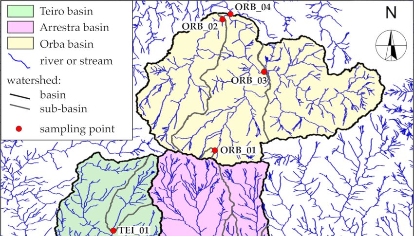
Geosciences 2019, 9, 258                                                                             2 of 22

dioxide by capturing more atmospheric CO2 through chemical weathering (higher temperatures and
rainfall accelerate mineral dissolution). We are still unaware of what is the response of weathering to
climate change at a global scale but it is clear that chemical weathering is also playing a significant role
in the short-term global carbon cycle and the mechanism of CO2 consumption by chemical weathering
should be considered in the future models of climate change [11].
     One of the most reliable ways of studying weathering reactions in natural settings is the
quantification of the mass fluxes into and out of watershed systems [12–17]. Natural chemical
weathering rates can be computed through accurate geochemical mass balances of river systems
following two complementary approaches: (i) the study of large river systems, that are currently used
for the estimation of the CO2 consumption by weathering at a global scale [15–23]; (ii) the study of
small mono lithology river basins that can give more accurate estimations of the chemical weathering
rates and their controlling parameters in natural settings [24–28].
     The knowledge of the relationships between natural chemical weathering rates and controlling
parameters (e.g., temperature, precipitation, infiltration, runoff) can help to clarify the discrepancy
observed between field and laboratory data [28–32] and could allow the up-scaling of local
measurements to a global scale, contributing to the refinement of global CO2 consumption estimations.
Furthermore, study of the parameters controlling weathering rates in natural settings can improve the
knowledge of the feedback between climate and weathering and its role on short-term carbon cycle
and climate change [10,11,23].
     The weathering of calcium and magnesium silicates is the main geologic mechanism naturally
limiting atmospheric CO2 levels. The weathering process transforms CO2 into bicarbonate, that in
the long term (time > 1 Ma) precipitates as Ca and Mg carbonate in the oceans. Ultramafic rocks,
almost completely composed by Mg, Fe, and Ca silicates, are the rocks with the highest potential for
the removal of CO2 from the atmosphere-hydrosphere system and their alteration process significantly
affected the evolution of the Earth’s atmosphere [33] and continental crust through geological times [34].
Despite the interest on ultramafic rocks for their potential use in the field of mineral carbonation [35,36]
and their importance for the study of the atmospheric evolution, the rate of CO2 uptake via weathering
of peridotite and serpentinite is still poorly known in natural conditions [37].
     In this work we investigate the chemical weathering of ultramafic rocks through the geochemical
and isotopic study of three small rivers whose drainage basins are almost completely composed of
the ultramafic rocks of the Voltri Massif, Western Alps–Northern Italy (Figure 1). The main objectives
of the work are (1) to estimate the natural chemical weathering rates, (2) to determine the rates of
atmospheric CO2 consumption related to chemical weathering, (3) to study the control exerted by
runoff, temperature, and other potential controlling factors on chemical weathering rates of ultramafic
rocks, and (4) to compare our results to the global estimations of CO2 consumption rates.

2. Study Area
     The study area is located in the Ligurian Alps few kilometers west of the city of Genoa (Northern
Italy) where the southern part of the Western Alps leave place to Appennines. It is bordered to the
south by the steep continental margin of the Liguro-Provençal Basin and to the north by the Neogene
thick sedimentary prism of the Po Plain (Figure 1a).
     The geology of the area is dominated by the Voltri Massif, a 30 km wide, E-W elongated
tectono-metamorphic unit [38,39]. The Voltri Massif, which has in the M. Beigua (1287 m asl) its
highest peak, belongs to the internal Penninic Units of the Western Alps and is located at the boundary
between Western Alps and Northern Apennines. It is separated from the Apennine chain by the
Sestri Voltaggio zone to the east and bordered to the south by the Ligurian sea and to the north by
the Tertiary sediments (continental to shallow marine breccias, conglomerates and sandstones) of
the Tertiary Piedmont Basin [40–43] and it is in contact to the west with the Hercynian continental
basement rocks of the Savona Massif [44]. The Voltri tectono-metamorphic unit corresponds to a
remnant of the oceanic lithosphere of the Jurassic Piedmont-Ligurian ocean subducted during plate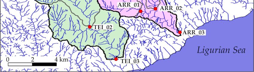
Geosciences 2019, 9, x FOR PEER REVIEW 3 of 22
Hercynian
Geosciences continental
2019, 9, 258 basement rocks of the Savona Massif [44]. The Voltri tectono-metamorphic 3 of 22
unit corresponds to a remnant of the oceanic lithosphere of the Jurassic Piedmont-Ligurian ocean
subducted during plate convergence between Europe and Adria [39,45–49]. It is composed of
convergence
metamorphicbetween Europe
ophiolitic andwith
rocks Adriaassociated
[39,45–49].metasediments
It is composed ofand metamorphic
slices of ophiolitic
lithosphericrocks with
mantle
associated metasediments and slices of lithospheric mantle placed at the top of the
placed at the top of the meta-ophiolite series (Figure 1b). Meta-ophiolites mainly consist of meta-ophiolite series
(Figure 1b). Meta-ophiolites
serpentinites, metagabbros,mainly consist of serpentinites,
and metabasites; metagabbros, and
associated metasediments metabasites;
comprise associated
calc-schists, and
metasediments
minor mica-schists and quartz-schists; mantle rocks include lherzolite and harzburgite andinclude
comprise calc-schists, and minor mica-schists and quartz-schists; mantle rocks minor
lherzolite
fractions ofand harzburgite
pyroxenite andand minor
dunite fractions of pyroxenite and dunite [39,43,45,46,50–54].
[39,43,45,46,50–54].
From
From lower
lower Eocene
Eocene until
until the
the Eocene–Oligocene
Eocene–Oligocene boundary
boundary the the Voltri
Voltri Massif
Massif experienced
experienced aa
complex
complex deformational evolution linked to different phases of the subduction–exhumation cycle
deformational evolution linked to different phases of the subduction–exhumation cycle of
of
the Alpine orogenesis [44,55], with metamorphic conditions evolving from eclogitic
the Alpine orogenesis [44,55], with metamorphic conditions evolving from eclogitic to greenschist to greenschist
facies
facies [39,54,56,57].
[39,54,56,57].
The
The late
late orogenic
orogenic evolution
evolution ofof the
the Ligurian
Ligurian Alps
Alps isis coeval
coeval with
with the
the deposition
deposition of of the
the Tertiary
Tertiary
Piedmont Basin sedimentary succession [40,42]. Its sedimentation occurred
Piedmont Basin sedimentary succession [40,42]. Its sedimentation occurred in the Oligo–Miocenein the Oligo–Miocene
when
when three
three main
main tectonic
tectonic episodes
episodes occurred:
occurred: the
the exhumation
exhumation of of the
the Ligurian
Ligurian sector
sector of
of the
the Western
Western
Alps, the opening of the Liguro-Provençal basin accompanied by the
Alps, the opening of the Liguro‐Provençal basin accompanied by the Corsica–SardiniaCorsica–Sardinia anticlockwise
rotation [58,59],rotation
anticlockwise and the[58,59],
formation
and of
thethe Apennines
formation [42].Apennines [42].
of the
Figure 1.
Figure 1. (a)
(a) Location
Locationofofthe
thestudy
studyarea;
area;(b)
(b)geo-lihological
geo-lihological map,
map, simplified
simplified from
from thethe litholgical
litholgical mapmap
of
of Regione Liguria
Regione Liguria [38]. [38].
The subsequent
The subsequent tectonic
tectonic extensional
extensional regimeregime (since early-middle
(since early-middle Miocene)
Miocene) caused caused the
the development
development
of a dense suiteofofanormal
dense faults
suite of normal
that shapedfaults that shaped the
the geomorphology of geomorphology of the study
the study area, defining area,
the current
defining
aspect of the current
coast andaspect of the coast of
the hypsometry and thecoastal
this hypsometry
sectionof ofthis coastal
Ligurian section of Ligurian Alps.
Alps.
Thegeomorphological
The geomorphological andand hydrological
hydrological features
features of theof theMassif
Voltri Voltrishow
Massif
some show some
marked marked
differences
differences
between the between
southern the
side,southern
draining side,
towarddraining toward
the Ligurian theand
Sea, Ligurian Sea, and
the northern side,the northern
draining side,
towards
draining towards the Po plain. The southern side of the massif is characterized
the Po plain. The southern side of the massif is characterized by steep slopes, streams with low by steep slopes,
streams with
sinuosity, low elongated
and N-S sinuosity, drainage
and N-S basins;
elongated drainageside
the northern basins; the northernbyside
is characterized is characterized
gentle slopes and a
by gentle
more slopes
complex and a more
drainage complex
network. Thedrainage
rapid upliftnetwork.
of the The rapid uplift
Thyrrenian of the
margin Thyrrenian
is the reason why margin
the
is the draining
basins reason why thethe
toward basins draining
Ligurian Sea aretoward
steeperthethanLigurian Sea aretoward
those draining steeperthethan thosewhere
Po Plain draining
the
toward
uplift the Po Plain
is hampered where
by the loadthe uplift
of the is hampered
Tertiary Piedmontby the sediments
Basin load of the Tertiary Piedmont Basin
[60].
sediments [60].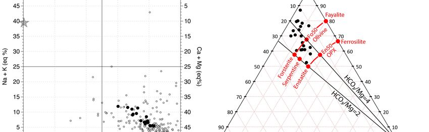
Geosciences 2019, 9, 258                                                                             4 of 22

    The study area is characterized by a long-period (30 years) averaged maximum temperature of 27
◦Cin August and a minimum of 6 ◦ C in January; the annual average rainfall is about 1250 mm with
two precipitation maxima in October and April and a minimum in July [61].

3. Materials and Methods

3.1. Theoretical Background
     Considering the paragenesis of the ultramafic rocks characterizing the study area [50,62], some
of the most relevant weathering reactions that affect river water composition and soil formation are:
dissolution of olivine (e.g., forsterite),

                           Mg2 SiO4 + 4CO2 + 4H2 O → 2Mg2+ + 4HCO3 − + H4 SiO4 ,                        (1)

dissolution of pyroxene (e.g., enstatite),

                           Mg2 Si2 O6 + 4CO2 + 6H2 O → 2Mg2+ + 4HCO3 − + 2H4 SiO4 ,                     (2)

serpentine dissolution,

                       Mg3 Si2 O5 (OH)4 + 6CO2 + 5H2 O → 3Mg2+ + 6HCO3 − + 2H4 SiO4 ,                   (3)

and alteration of anorthite to kaolinite,

                       CaAl2 Si2 O8 + 2CO2 + 3H2 O → Al2 Si2 O5 (OH)4 + 2HCO3 − + Ca2+                  (4)

    In the study area some reactions involving the rocks of the metasedimentary cover (where present)
may occur, such as the alteration of muscovite and feldspars to hydroxides and/or clay minerals (e.g.,
muscovite to kaolinite),

               2KAl2 (Si3 Al)O10 (OH)2 + 5H2 O + 2CO2 → 3Al2 Si2 O5 (OH)4 + 2K+ + 2HCO3 − ,             (5)

and the congruent dissolution of calcite

                                   CaCO3 + H2 O + CO2 → Ca2+ + 2HCO3 − .                                (6)

      Chemical weathering of silicates and carbonates consumes atmospheric/soil carbon dioxide,
causes the increase of alkalinity and the increase of dissolved cations and silica in the solution. For each
reaction, the moles of atmospheric/soil CO2 consumed by the weathering of one mole of mineral can be
computed from the concentration of cations in solution, considering the stoichiometry of the reactions.
For the Equations (1) to (4), the molal ratio between consumed CO2 and divalent cations in solution is
2. Similar reactions, showing the same molal ratio between cations in solution and consumed CO2 ,
could be written for most of the silicates containing calcium, magnesium and ferrous iron. For the
reactions involving silicates with monovalent cations (e.g., Equation (5)) and carbonates (e.g., Equation
(6)) the molal ratio between consumed CO2 and cations in solution is 1.
      On the long term (>1 Ma), part of the atmospheric carbon consumed by weathering is returned
to the atmosphere through several processes: (i) the CO2 consumed by weathering of carbonates
in the continents is completely returned to the atmosphere through carbonate precipitation in the
ocean (reverse of Equation (6)); (ii) half of the CO2 consumed during weathering of Ca and Mg
silicates is precipitated as CaCO3 and half is released back into the atmosphere as CO2 ; (ii) Na+ and K+
ions, transported by rivers to the ocean, may undergo reverse weathering to form authigenic clays
and CO2 [63]. As a result, while on the short term both carbonate and silicate weathering consume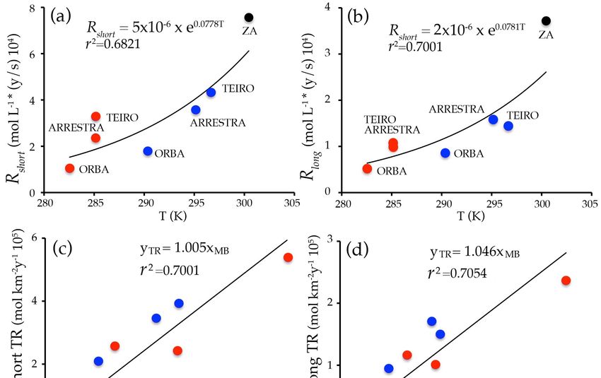
Geosciences 2019, 9, 258                                                                                                5 of 22
Geosciences 2019, 9, x FOR PEER REVIEW                                                                                 5 of 22

atmospheric COFCO2 , on the long
                      2-short    term
                              = FNa  sil +only
                                           FKsilweathering
                                                + 2FMgsil + FMgof Ca
                                                                   carband  Mgsilsilicate
                                                                        + 2FCa       + FCacarbminerals
                                                                                               + 2FFesilis
                                                                                                         , a net sink (7)
                                                                                                                      for
atmospheric/soil CO2 [8,23,62].
      Considering the stoichiometric FCO    2-long = FMg
                                          coefficients     sil + FCasil +(1)
                                                        of Equations      FFetosil,(6), it is possible to compute two (8)
different
where  FCOmass  balance equations relating atmospheric/soil CO2 consumption
            2-short and FCO2-long are the fluxes of atmospheric
                                                                                                 to the composition
                                                                                     carbon dioxide       consumed by  of
river waters. The first equation is related    to short term   carbon   cycle  and     the  second
weathering in the short and long term, FX is the flux of a generic cation X, given by its molal     is for the long term:
concentration multiplied by the runoff, and the suffixes sil and carb stand for silicate and carbonate,
                 FCO2 -short = FNasil + FKsil + 2FMgsil + FMgcarb + 2FCasil + FCacarb + 2FFesil ,                           (7)
indicating the origin        of the dissolved chemical species.
       The application of the mass balances (7) and (8) are based on the assumption that carbonic acid
                                           FCO2 -long = FMgsil + FCasil + FFesil ,                                          (8)
is the only source of protons in the weathering reactions and that the contribution related to
 where FCO
sulphide        2 -short and
             minerals          FCO2 -long
                          oxidation          are the fluxes
                                       is negligible.         of atmospheric
                                                         In addition,           carbon dioxide
                                                                        it is important    to noteconsumed     by weathering
                                                                                                      that dissolved  iron in
 in  the  short    and   long   term,  FX   is the  flux   of a  generic   cation   X,  given
surface water is often fixed at very low concentrations by oxides/hydroxides precipitation and by   its molal  concentration
 multipliedthe
therefore       by measured
                     the runoff, concentrations
                                   and the suffixescouldsil andbecarb
                                                                   anstand     for silicate and
                                                                        underestimation      of carbonate,     indicating
                                                                                                  the total amount      of the
                                                                                                                            Fe
 origin of from
deriving     the dissolved      chemical species.
                    silicate weathering.
        The application of the mass balances (7) and (8) are based on the assumption that carbonic acid is
3.2.
 the Phases    of the Study
      only source      of protons in the weathering reactions and that the contribution related to sulphide
 minerals oxidation is negligible. In addition, it is important to note that dissolved iron in surface water
       In this work the relationships among dissolved loads, natural weathering rates and CO2
 is often fixed at very low concentrations by oxides/hydroxides precipitation and therefore the measured
consumed by weathering reactions are investigated in three streams whose drainage basins are
 concentrations could be an underestimation of the total amount of Fe deriving from silicate weathering.
mainly composed by the ophiolites of the Voltri Massif (Figure 2). Two streams (Teiro and Arrestra)
run    southward
 3.2. Phases    of the towards
                        Study      the Ligurian Sea and the third one (Orba) runs northwards up to its
confluence with the Bormida river, a right tributary of the Po river.
        In this
       The       work
             study      thebeen
                      has    relationships
                                  carried outamong     dissolved
                                                 in three   steps:loads,   natural weathering
                                                                    (i) definition                 rates and
                                                                                     of the hydrologic,       CO2 consumed
                                                                                                            geographic,   and
 by  weathering      reactions   are investigated     in three  streams   whose    drainage   basins
geologic features of the studied basins and subdivision of the main drainage basins in smaller sub-     are mainly composed
 by the using
basins     ophiolites
                    a GIS of the  Voltri
                              based       Massif (Figure
                                      approach,               2). Two
                                                    (ii) stream          streamschemical
                                                                    sampling,       (Teiro andandArrestra)
                                                                                                     isotopicrun  southward
                                                                                                                analyses  (iii)
 towards     the   Ligurian     Sea and   the  third   one   (Orba)   runs  northwards      up
geochemical mass balance and estimation of natural weathering rates and CO2 consumption rates   to  its  confluence  with  the
 Bormida     river,   a right  tributary
based on the Equations (7) and (8).       of  the Po   river.

                           Figure
                           Figure 2.
                                  2. Drainage
                                     Drainagebasins
                                              basinsand
                                                     andlocation
                                                         locationof
                                                                 ofthe
                                                                    thesampling
                                                                        sampling points.
                                                                                 points.

3.3. Definition of the Drainage Basins
   Teiro and Arrestra streams are characterized by NW-SE elongated catchments with very steep
morphologies, on the contrary the drainage basin of the Orba stream, draining on the opposite side
Geosciences 2019, 9, 258                                                                                         6 of 22

     The study has been carried out in three steps: (i) definition of the hydrologic, geographic, and
geologic features of the studied basins and subdivision of the main drainage basins in smaller sub-basins
using a GIS based approach, (ii) stream sampling, chemical and isotopic analyses (iii) geochemical
mass balance and estimation of natural weathering rates and CO2 consumption rates based on the
Equations (7) and (8).

3.3. Definition of the Drainage Basins
     Teiro and Arrestra streams are characterized by NW-SE elongated catchments with very steep
morphologies, on the contrary the drainage basin of the Orba stream, draining on the opposite side of
the watershed, is characterized by a relatively gentle morphology after a steep descent just behind the
main divide. The elevation of the studied areas ranges from a few meters above sea level up to the 1287
m above sea level (a.s.l.) of Monte Beigua. The three drainage basins and other derived parameters
(Figure 2) were defined from the 5 m spatial resolution Digital Terrain Model of the Regione Liguria [63].
Each drainage basin was further subdivided in different sub-basins: Teiro basin was subdivided in
three sub-basins following a nested pattern, where each sub-basin is completely contained in the
downstream sub-basin; Arrestra basin and Orba basin were subdivided in three and four sub-basins
respectively, following an additive pattern, where each sub-basin, except for the lowest one, is not
spatially connected to the others, eventually sharing just a divide with the adjacent sub-basins. To be
more precise while Teiro 3 contains Teiro 2, that contains Teiro 1 (nested patterns), Arrestra 3 contains
both Arrestra 2 and Arrestra 1, but Arrestra 2 does not contain Arrestra 1 (additive pattern). In any case,
the outlet of the lowest sub-basin (Teiro 3, Arrestra 3, and Orba 4) drains the totality of the basin area.
     For each basin and sub-basin, the morphological parameters as surface area, average elevation
and statistics were computed using GRASS GIS 7.6 packages [64]. The main features of the three basins
are reported in Table 1.

                           Table 1. Surface area and average elevation of drainage sub-basins.

                                                                         Mean              Minimum      Maximum
     Drainage
                           Sub-Basin 1         Surface (km2 )          Elevation           Elevation    Elevation
      Basin
                                                                        (m a.s.l)           (m a.s.l)    (m a.s.l)
       Teiro                 Teiro 1                  2.9                  843                  370       1287
       Teiro                 Teiro 2                 14.6                  665                  100       1287
       Teiro                 Teiro 3                 26.5                  487                   10       1287
      Arrestra              Arrestra 1               11.7                  741                  171       1287
      Arrestra              Arrestra 2                4.7                  677                  139       1145
      Arrestra              Arrestra 3               20.0                  632                   20       1287
       Orba                  Orba 1                   0.2                 1137                 1081       1198
       Orba                  Orba 2                  10.7                  939                  730       1287
       Orba                  Orba 3                  14.6                  915                  610       1181
       Orba                  Orba 4                  39.6                  919                  540       1287
                                1   The hierarchy of sub-basins is graphically shown in Figure 2.

     The relative abundances of outcropping rocks in the three drainage basins were computed
with GRASS, extracting the data from the simplified geo-lithological map (Figure 1) derived from
a multi-source geological map of Regione Liguria [38]; the results (Table 2) show that the Arrestra
and the Orba basins are characterized by the prevalence of serpentinites, metagabbros, and eclogites
while the Teiro basin shows a greater heterogeneity with a relevant fraction of metasedimentary
rocks (mainly calc-schists) alternating with ultramafic meta-ophiolites. Post-orogenic sedimentary
deposits (conglomerates) are negligible and in any case the constituent material is principally made by
bedrock lithotypes.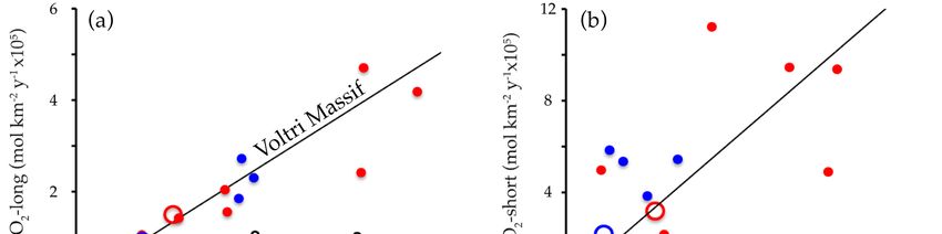
Geosciences 2019, 9, 258                                                                                         7 of 22

      Table 2. Relative abundance (surface area %) of the rock types outcropping in the ten sub-basins
      considered in this work, grouped starting from the map of Figure 1b.

    Sub-Basin              Peridotites       Metabasites *        Serpentinite        Calc-Schistes   Conglomerates
      Teiro 1                  0.0                10.3                 41.4                 48.3           0.0
      Teiro 2                  0.0                12.4                 47.6                 36.6           3.4
      Teiro 3                  0.0                14.0                 43.4                 36.2           6.4
     Arrestra 1                0.9                10.3                63.9                  24.8           0.0
     Arrestra 2                0.0                 4.3                93.6                   2.1           0.0
     Arrestra 3                0.5                12.5                71.8                  14.9           0.0
      Orba 1                   0.0                 0.0                100.0                  0.0           0.0
      Orba 2                   0.0                12.1                 78.5                  9.3           0.0
      Orba 3                   0.0                13.7                 84.2                  2.1           0.0
      Orba 4                   0.0                13.4                 81.6                  5.1           0.0
                               * Metabasites includes metagabbros, eclogites, and amphibolites.

3.4. Sampling and Analyses
     Ten sampling sites were selected for this study, located near the sub-basin outlets (three in the
Arrestra basin, three in the Teiro basin, and four in the Orba basin) (Figure 2). Sampling was performed
twice, during the dry (July 2016) and wet (April 2017) seasons, for a total of twenty samples. Also
measured on each sampling site was the stream discharge (Q) using the velocity-area method.
     For each sample, temperature, electrical conductivity, pH, Eh, and dissolved oxygen (DO) were
measured in the field with a laboratory pre-calibrated HANNA HI 9829 multiparameter meter (electrical
conductivity: resolution = 1 µS/cm, accuracy = ±1%; pH: resolution = 0.01, accuracy = ±0.02 pH; Eh:
resolution = 0.1 mV, accuracy = ±0.5 mV; DO: resolution = 0.01 mg/L, accuracy = ±1%). Total and
carbonate alkalinity were determined in the field on a fresh water sample with digital titrator HACH
16900 by acid titration with H2 SO4 0.16 N on 25 mL of water using Phenolphthalein and Bromochresol
Green-Methyl Red as indicators.
     Water samples for chemical analyses were filtered with 0.45 µm filters and collected in three 50 mL
polyethylene bottles. One aliquot was immediately acidified with 0.5 mL of concentrated suprapure
HCl in order to stabilize the sample, preventing algal growth and carbonate precipitation. A second
aliquot was acidified with 0.5 mL of ultrapure HNO3 to avoid precipitation of metals as metal oxides
or hydroxides. A further sample for the determination of the isotopic composition of water (δD, δ18 O)
was collected in a 100 mL polyethylene bottle preventing the formation of head space. Finally, for the
determination of δ13 C of total dissolved inorganic carbon (δ13 CTDIC , TDIC), all the dissolved carbon
species were precipitated in the field as SrCO3 by adding an excess of SrCl2 and NaOH to 1000 mL of
water. In the laboratory carbonate precipitates were filtered, washed with distilled water, and dried in
a CO2-free atmosphere.
     All the chemical determinations were performed at the Geochemical Laboratory of the Perugia
University. Sulphate, NO3 − , Cl− , and F− were determined by ion-chromatography (Dionex DX120
with AS50 autosampler). Ca and Mg concentrations were determined by atomic absorption flame
spectrometry (IL951 AA/AE), using the HCl acidified sample for the determination of Ca, while Na
and K were determined by atomic emission flame spectrometry (IL951 AA/AE). Low range protocol
analyses for Al and silica were determined by UV/Vis spectrophotometry (HACH DR2010), using
Eriochrome Cyanine R and silicomolybdate methods respectively. The detection limits are: 0.01 mg/L
for Ca, Mg, Na, K, F− , and NO3 − , 0.03 mg/L for Cl− and SO4 2− , 4 µg/L for Al, 5 µg/L for total iron, and
0.45 mg/L for SiO2 .
     All the laboratory analytical methods and the field alkalinity determinations have an accuracy
better than 2%. The total analytical error, evaluated checking the charge balance, is about 0.8% on
average, and is lower than 3% for all the samples.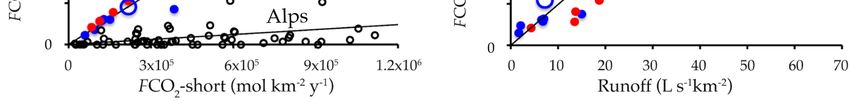
Geosciences 2019, 9, 258                                                                             8 of 22

      The analyses of the hydrogen and oxygen stable isotope ratios were performed at the isotope
laboratory of Parma University using a Thermo Delta Plus mass spectrometer and the isotope analyses
of TDIC were performed by means of standard mass spectrometry techniques using a Delta S mass
spectrometer at CNR-IGG, Section of Florence. The values of δD and δ18 O are referred as δ (%) of the
standard SMOW. The values of δ13 C are referred as δ (%) of the standard PDB. Analytical errors are:
±1% for δD, ±0.1% for δ18 O, and δ13 C.
      The location of the sampling points is shown in Figure 2, field data are in Table S1 and the results
of isotopic and chemical analyses are listed in Table S2.

3.5. Computation of Runoff, Solute Flux, Weathering Rates, and CO2 Consumption Rates
     For each drainage basin and sub-basin, we computed (i) the runoff, given by the ratio between
streamflow (Q) and surface area, (ii) the flux of dissolved solids, given by the product of total dissolved
solids (TDS) by runoff, (iii) the weathering rate, calculated from the difference between TDS and the
atmospheric/biologic components multiplied by runoff, and (iv) FCO2 -short and FCO2 -long, from
Equations (7) and (8).
     For the estimation of the weathering rates and CO2 consumption rates it was first necessary to
subtract the rain/atmospheric contribution to the stream waters composition [23,65]. Assuming that
chloride in stream waters derive entirely from the rain/atmospheric input, the concentration of each
ion (X) has been corrected using the ion to chloride molal ratios in rainwater,

                                   Xcorr = Xstream − Clstream ∗(X/Cl)rain ,                             (9)

where Xcorr is the ion concentration after the correction for the rain/atmospheric contribution and the
suffixes stream and rain stand for stream water and rainwater. Calculations were performed considering
the average the X/Cl molal ratios in rainwaters of the northern Mediterranean area and Ligurian
sea [66,67].
     For some sub-basins (see next section) it was also necessary to discriminate the fraction of Ca
deriving from silicate weathering from the fraction deriving from calcite dissolution (Casil and Cacarb
in Equations (7) and (8)). The Ca/Mg molal ratio (0.59) of the waters sampled in the Orba basin and
Arrestra 2 sub-basin, where the amount of calcite is negligible (Table 2), has been considered to be
representative of the interaction of stream water with ultramafic rocks. The amount of Ca deriving
from calcite dissolution was then computed for each sample from:

                                        Cacarb = Ca − 0.59Mgsil .                                     (10)

4. Results

4.1. Chemical and Isotopic Composition of Stream Waters
     The stream waters of the study area, during the July 2016 campaign, were characterized by
temperatures between 19.1 and 28.6 ◦ C, pH from 5.79 to 8.98 with a mean value of 8.03, electrical
conductivity (EC) from 80 to 315 µS with a mean value of 177 µS/cm, average dissolved oxygen (DO)
of 7.24 ± 0.83 mg/L, and an average Eh of 210 ± 22 mV. The same streams, during the April 2017
campaign, were characterized by temperatures between 7.8 and 13.8 ◦ C, pH values from 7.54 to 9.17
(mean value = 8), EC values from 70 to 250 µS/cm (mean value = 136 µS/cm), average DO = 10.11 ±
1.18 mg/L and average Eh = 236 ± 25 mV.
     The values of pH did not show any significant change between the two campaigns, while EC, total
dissolved solids (TDS—computed from analyses), DO and Eh showed significant seasonal variations.
EC decreased of almost 25% from the July 2016 campaign (dry season) to the April 2017 campaign (wet
season). Similarly, also TDS values were higher for the samples taken during the dry season (mean of
July 2016 campaign TDS = 116 ± 50 mg/L; mean of April 2017 campaign TDS = 88 ± 36 mg/L). These
variations of EC and TDS are likely caused by the dilution effect of rainwater during the wet season.
Geosciences 2019, 9, 258 9 of 22
Conversely, DO and Eh values increased from the dry to the wet season probably because oxygen
solubility in water increases as temperature decreases (e.g., at 1 bar and 25 ◦ C, air-saturated water
would hold 7.7 mg/L of dissolved oxygen, while at 1 bar and 5 ◦ C there would be 9.7 mg/L of dissolved
oxygen at 100% air saturation).
In the diagram δ18 O vs. δD (Figure 3) the stream waters of the study area plot between the global
meteoric water line (GMWL [68]) and the meteoric water line of the Mediterranean area (MMWL [69]),
indicating that the precipitations in the Voltri Massif derive both from weather fronts originating north
Geosciences 2019, 9, x FOR PEER REVIEW 9 of 22
of the European continent, in the Atlantic Ocean, and weather fronts coming from the Mediterranean
Sea. Furthermore,
that dissolutionstream waters plot
of serpentine and close
other to the groundwaters
mafic minerals is theof the Voltri
main Massif [70]
water-gas-rock and do not
interaction
showprocess
any evident isotopic shift due to
occurring in the studied waters. evaporation.
Figure
Figure 3. δD3.vs. 18δ
δD δvs O18O diagram.The
diagram. Thestream
stream waters
waters are
arecompared
comparedtotothe global
the meteoric
global water
meteoric lineline
water (δD (δD
= 8 δ18O + 10 [68]) and to the Mediterranean meteoric water line (δD = 8 δ1818O + 22 [69]).
= 8 δ O + 10 [68]) and to the Mediterranean meteoric water line (δD = 8 δ O + 22 [69]). In the same
18 In the same
diagram
diagram are reported
are reported alsoalso
thethe groundwatersofofthe
groundwaters theVoltri
VoltriMassif
Massif [70].
[70].
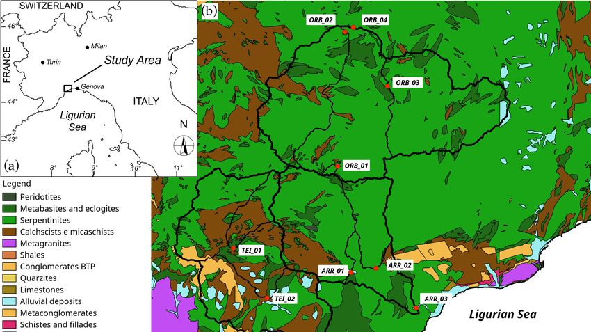
The Langelier–Ludwig diagram (Figure 4a) shows that all the samples are characterized by
a bicarbonate-earth alkaline composition similar to the composition of groundwaters of the Voltri
Massif [67]. The salinity (46 < TDS < 205 mg/L) is lower, on average, than the rivers of the Alpine
region (96 < TDS < 551 mg/L [23]). Consistently with the composition of the outcropping rocks, the
Mg concentration is relatively high and the Mg/Ca molal ratio varies from 0.18 to 1.56 suggesting
that dissolution of serpentine and other mafic minerals is the main water-gas-rock interaction process
occurring in the studied waters.
In the trilinear Mg-SiO2 -HCO3 plot of Figure 4b, the samples are compared to the theoretical
composition of solutions deriving from the dissolution of serpentine, olivine and pyroxene according
to Equations (1) to (3). For the dissolution of pure Mg-silicates (e.g., serpentine, enstatite, forsterite) the
theoretical solutions plots along the line HCO3 /Mg = 2, for silicates containing other divalent cations
in addition to Mg, the solutions are characterized by an higher HCO3 /Mg molal ratio (for example
the solution obtained from dissolution of the Fo50 -Fa50 term of the olivine series is characterized by
HCO3 /Mg = 4). About 45% of the samples fall between the HCO3 /Mg = 2 and HCO3 /Mg = 4 lines and
below theFigure
curve4.characterized 3 /SiO2 = 4, representing olivine dissolution. The composition
(a) Langelier–Ludwig
by a HCOdiagram showing the sampled stream waters (black dots) and 375
groundwaters of the Voltri Massif
of these waters if fully explained by dissolution(white dots
of [70]). For reference,
serpentine and/ormean
otherseawater composition
Mg-bearing is About
silicates.
plotted as a grey star. (b) Trilinear Mg-SiO2-HCO3 plot based on molal composition: the composition
55% of the data show a HCO3 /SiO2 higher than the olivine dissolution ratio. In order to explain the
of stream waters (black dots) are compared to composition of theoretical solutions deriving from
composition of these samples is necessary to consider some additional processes together with the
dissolution of some relevant mafic minerals (red dots). The red lines represent the olivine and
orthopyroxene series. The HCO3/Mg = 2 line represents the solutions resulting from dissolution of
pure Mg silicates while the HCO3/Mg = 4 line represents the solutions deriving from dissolution of
silicates where Mg is 50% of the divalent cations.
In the trilinear Mg-SiO2-HCO3 plot of Figure 4b, the samples are compared to the theoretical
composition of solutions deriving from the dissolution of serpentine, olivine and pyroxeneGeosciences 2019, 9, 258 10 of 22
Figure 3. δD vs δ18O diagram. The stream waters are compared to the global meteoric water line (δD
dissolution= 8ofδ18Mg-silicates. Plausible
O + 10 [68]) and processes are
to the Mediterranean the alteration
meteoric water line of
(δDaluminosilicates
= 8 δ18O + 22 [69]). and the
In the congruent
same
dissolutiondiagram are reported also the groundwaters of the Voltri Massif [70].
of carbonates.
4. (a)4.Langelier–Ludwig
FigureFigure (a) Langelier–Ludwig diagram showing
diagram showingthe the sampled streamwaters
sampled stream waters(black
(black dots)
dots) andand375375
groundwaters
groundwaters of theofVoltri
the Voltri
MassifMassif
(white(white dots [70]).
dots [70]). For reference,
For reference, meanmean seawater
seawater composition
composition is
is plotted
plotted as a grey star. (b) Trilinear Mg-SiO -HCO plot based on molal composition: the
as a grey star. (b) Trilinear Mg-SiO2 -HCO3 plot based on molal composition: the composition of stream
2 3 composition
watersof(black
streamdots)
waters
are(black
compared dots) to
arecomposition
compared toofcomposition
theoreticalof theoretical
solutions solutions
deriving fromderiving from of
dissolution
some relevant mafic minerals (red dots). The red lines represent the olivine and orthopyroxeneand
dissolution of some relevant mafic minerals (red dots). The red lines represent the olivine series.
orthopyroxene series. The HCO3/Mg = 2 line represents the solutions resulting from dissolution of
The HCO3 /Mg = 2 line represents the solutions resulting from dissolution of pure Mg silicates while
pure Mg silicates while the HCO3/Mg = 4 line represents the solutions deriving from dissolution of
the HCO3 /Mg = 4 line represents the solutions deriving from dissolution of silicates where Mg is 50%
silicates where Mg is 50% of the divalent cations.
of the divalent cations.
In the trilinear Mg-SiO2-HCO3 plot of Figure 4b, the samples are compared to the theoretical
In order to assess the sources and processes controlling stream chemistry, aqueous speciation and
composition of solutions deriving from the dissolution of serpentine, olivine and pyroxene
saturation index (SI) calculations have been performed with the PHREEQC geochemical code [71]
using the “llnl” database [72]. All the samples are strongly undersaturated with respect to the minerals
of the serpentine, olivine and pyroxene groups (saturation indexes ranging from −5 to −70) indicating
that their dissolution is an irreversible process. Saturation indexes of secondary minerals and carbon
dioxide partial pressure (Table 3) show that:
- all the samples are saturated or supersaturated with respect to amorphous Fe(OH)3 and goethite,
suggesting that Fe oxyhydroxides control the iron concentration in solution;
- the samples of the Arrestra and Orba streams are supersaturated with respect to illite, kaolinite, and
clay minerals of the smectite group (e.g., montmorillonite), close to equilibrium or supersaturated
with respect to gibbsite and quartz (but undersaturated with respect to amorphous silica) and
undersaturated with respect to calcite, dolomite, magnesite and brucite;
- the samples of the Teiro stream show extremely variable saturation conditions for clay minerals
and quartz, are generally undersaturated with respect to gibbsite, brucite, and magnesite (except
for Teiro 3 samples), close to equilibrium or supersaturated with respect to calcite (in particular
during the July 2016 survey) and supersaturated with respect to ordered dolomite;
- the logarithm of carbon dioxide partial pressure (log10 pCO2 ) vary within a relatively small
interval, from −4.27 to −2.88, following a log-normal distribution (Figure 5). Its probability
distribution is characterized by a mean of −3.37 (10−3.37 bar) and a median of −3.30 (10−3.30 bar),
very close to the value of equilibrium with the atmospheric carbon dioxide (10−3.39 bar assuming
a CO2 concentration in atmosphere of 405 ppm), and suggests that most of the dissolved inorganic
carbon derive from the atmosphere. This hypothesis is supported also by the isotopic composition
of TDIC (−14.27 ≤ δ13 CTDIC ≤ −6.59) that is consistent with an atmospheric origin (δ13 Catm ≈ −8)
of dissolved carbon with a minor contribution of soil CO2 deriving from organic matter oxidation
(δ13 Corg ≈ −28).Geosciences 2019, 9, 258 11 of 22
Table 3. Log10 of the partial pressure of CO2 and saturation indexes.
Log10 Dol. Dol. SiO2
ID Caclite. Magn. Brucite Gibbsite Qz Montm. Kaol. Illite Goeth. Fe(OH)3
pCO2 ord. dis. am.
July 2016
Arr. 1 −2.88 −0.34 0.36 −1.39 −0.94 −4.35 0.27 0.25 −1.05 1.94 1.74 1.09 nc nc
Arr. 2 −3.14 −0.96 −0.44 −2.02 −1.14 −4.37 0.00 0.47 −0.84 2.35 1.63 1.06 nc nc
Arr. 3 −3.18 −0.21 0.88 −0.67 −0.55 −3.60 0.22 0.52 −0.77 3.30 2.18 2.30 6.43 0.58
Teiro 1 −3.43 0.06 0.77 −0.83 −0.97 −4.05 −0.29 −0.32 −1.66 −1.14 −0.55 −1.90 nc nc
Teiro 2 −3.40 0.34 1.52 −0.03 −0.46 −3.30 nc 0.22 −1.08 nc Nc nc nc nc
Teiro 3 −3.92 1.10 3.39 1.67 0.48 −1.69 −0.98 0.20 −1.05 1.04 −0.82 −0.33 6.34 0.38
Orba 1 −3.26 −1.89 −2.60 −4.22 −2.41 −5.83 nc 0.37 −1.00 nc Nc nc 6.96 1.48
Orba 2 −3.23 −1.23 −1.10 −2.70 −1.55 −4.84 0.51 0.48 −0.87 2.96 2.62 1.97 6.58 0.95
Orba 3 −3.31 −1.60 −1.65 −3.26 −1.73 −4.95 0.25 0.25 −1.10 1.55 1.64 0.73 nc nc
Orba 4 −3.11 −1.23 −1.13 −2.72 −1.57 −4.91 0.21 0.41 −0.92 2.18 1.91 1.13 6.54 0.87
April 2017
Arr. 1 −3.29 −0.80 −0.57 −2.21 −1.48 −5.01 0.36 0.48 −0.92 2.60 2.27 1.59 nc nc
Arr. 2 −3.31 −1.08 −0.78 −2.42 −1.41 −4.90 0.35 0.64 −0.75 3.31 2.59 1.98 6.70 1.29
Arr. 3 −2.98 −1.09 −0.99 −2.64 −1.62 −5.43 0.60 0.33 −1.07 2.18 2.44 1.43 6.69 1.27
Teiro 1 −3.62 −0.27 0.11 −1.54 −1.34 −4.60 0.56 0.53 −0.88 3.33 2.76 2.70 nc nc
Teiro 2 −3.84 −0.17 0.51 −1.13 −1.03 −4.00 −0.18 −0.06 −1.45 0.05 0.12 −0.77 nc nc
Teiro 3 −4.27 0.94 2.75 1.13 0.11 −2.33 −0.95 0.17 −1.21 0.53 −0.94 −0.82 nc nc
Orba 1 −3.39 −1.68 −2.69 −4.37 −2.75 −6.33 0.80 −1.57 −0.14 0.17 1.88 0.00 nc nc
Orba 2 −3.17 −1.85 −2.48 −4.14 −2.36 −6.10 1.12 0.63 −0.78 3.95 4.09 3.04 7.06 1.74
Orba 3 −3.23 −1.80 −2.33 −3.99 −2.25 −5.91 1.44 −0.20 −1.61 1.25 3.07 1.20 nc nc
Orba 4 −3.39 −2.29 −3.06 −4.72 −2.50 −6.02 1.08 0.51 −0.90 3.43 3.76 2.89 6.76 1.43
nc = not computable.Geosciences 2019, 9, 258 12 of 22
Geosciences 2019, 9, x FOR PEER REVIEW 12 of 22
Figure5.5. Histogram
Figure Histogramof
oflog
log10
10 pCO 2..
2
In
A the study
further area the
process to stream waters is
be discussed interact with ultramafic
the possible interaction rocks and ultramafic
of stream waters with soils,brucite.
whose
mineralogical
Brucite is a common compositionmineral is in
mostly inheritedperidotite
serpentinized from the parent rockworks
and recent (serpentine, olivine,that
demonstrate pyroxene)
often it
with
is theminor
fastestauthigenic
dissolvingspecies mineral, (clay
andminerals, Fe and Alother
might dominate oxyhydroxides)
processes [77,78]. and a low Bruciteorganic matter
dissolution
content [73]. Irreversible,
also increases congruentstate
the water saturation dissolution of Mg-silicates,
with respect to hydrated under Mg pCO 2 conditions
carbonate minerals close
[78]toand
the
atmospheric
both dissolution value, andisprecipitation
the major process producing
of brucite the observed
might affect chemical of
the computation compositions of stream
the CO2 consumption
waters. However,
flux. However, onlyconsidering
very minor that for Mg-silicates’
amounts of brucite dissolution
are present the in themaximum possible value
Voltri serpentinites andoftheir
the
HCO 3 /SiO2on
influence molal
the ratio in solution
composition of isriver
4 (corresponding to the congruent
waters is negligible. This dependsdissolution on of theolivine), in
tectonic-
order to explain
metamorphic the composition
evolution of the samples
of the ultramafic rocks ofwith Voltri3 /SiO
the HCO Massif:
2 > 4 it
duringis necessary
the ocean to hypothesize
stage of their
the occurrence
evolution, of an additional
the seafloor hydration process
led to such as incongruent
widespread dissolution
serpentinization of aluminosilicates,
of peridotites where
with formation
the precipitation
of chrysotile and of clay minerals
lizardite causes with
in association the relative
magnetite increase
and locally HCO3 /SiO
of the brucite [51,79];
2 ratio in solution.
subsequently,
Furthermore, for the samples of the Teiro
during the subduction–exhumation cyclestream,
of the characterized by very high
Alpine orogenesis HCO
[44,55], 3 /Mg ratiosrocks
ultramafic and
equilibrium
experienced with calcite, also the
a high-pressure dissolution
event during of calcium
which carbonate
brucite has to be considered.
was consumed with the formation of
The samples
metamorphic olivine of intheequilibrium
Teiro stream withare also strongly
antigorite, diopside,oversaturated
Ti-clinohumite, withand respect
fluidsto[79].
ordered
As a
dolomite
result, only [74,75], but, despite
very minor amounts this,
of the concentration
brucite are presentofinMg the in solution
Voltri is not limited
serpentinites. by dolomite
Furthermore, also
precipitation.
in the recent carbonateIn fact, at low temperature
deposits associated with and low salinity, primary
the ultra-alkaline springsprecipitation
of the area,ofbrucite
dolomite is
is not
extremely
present, as slowwell even asathydromagnesite
high supersaturations and is practically
and other hydrated Mg inhibited by reaction
carbonates [80]. kinetics [76].
The chemical
A furtherofprocess
composition to be discussed
river waters is the with
are consistent possible
theseinteraction of stream
observations: waters saturation
(1) brucite with brucite. Brucite
index are
is a common
always very mineral
negativein(Tableserpentinized peridotite
3) excluding and recent works
the possibility demonstrate
of brucite precipitation;that often it is the waters
(2) stream fastest
dissolving mineral,by
are characterized andthemight
Mg/SiO dominate
2 ratiosother processes [77,78].
of Mg-silicates or lower Brucite
(Figure dissolution
4) suggesting also increases
that brucitethe
water saturation
dissolution doesstatenot with
affectrespect to hydrated
significantly Mg carbonate
the composition ofminerals [78] andinboth
stream waters; fact,dissolution
if there wereand
precipitation of brucite
brucite dissolution, might waters
stream affect the computation
would of the 2CO
have Mg/SiO consumption
ratios
2 higher thanflux. However,
those of only very
Mg-silicates
minor amounts
dissolution andof thebrucite
samplesare would
presentshift
in the Voltri serpentinites
towards the lower left and their(Mg)
corner influence
in the ontrilinear
the composition
diagram
of river
Figure waters
4. is negligible. This depends on the tectonic-metamorphic evolution of the ultramafic
rocks of the Voltri Massif: during the ocean stage of their evolution, the seafloor hydration led to
4.2. Runoff, Solute
widespread Fluxes, Weathering
serpentinization Rates, and
of peridotites withCOformation
2 Fluxes of chrysotile and lizardite in association
with The
magnetite
results of the mass-balance calculations are summarized the
and locally brucite [51,79]; subsequently, during subduction–exhumation
in Table 4. cycle
of the Alpine orogenesis [44,55], ultramafic rocks experienced a high-pressure event during which
brucite was consumed with the formation of metamorphic olivine in equilibrium with antigorite,
diopside, Ti-clinohumite, and fluids [79]. As a result, only very minor amounts of brucite are present
in the Voltri serpentinites. Furthermore, also in the recent carbonate deposits associated with the
ultra-alkaline springs of the area, brucite is not present, as well as hydromagnesite and other hydrated
Mg carbonates [80]. The chemical composition of river waters are consistent with these observations:
(1) brucite saturation index are always very negative (Table 3) excluding the possibility of bruciteGeosciences 2019, 9, 258 13 of 22
precipitation; (2) stream waters are characterized by the Mg/SiO2 ratios of Mg-silicates or lower
(Figure 4) suggesting that brucite dissolution does not affect significantly the composition of stream
waters; in fact, if there were brucite dissolution, stream waters would have Mg/SiO2 ratios higher than
those of Mg-silicates dissolution and the samples would shift towards the lower left corner (Mg) in the
trilinear diagram of Figure 4.
4.2. Runoff, Solute Fluxes, Weathering Rates, and CO2 Fluxes
The results of the mass-balance calculations are summarized in Table 4.
Table 4. Runoff, solute flux, chemical weathering rates and fluxes of atmospheric CO2 consumed
by chemical weathering considering both the short and the long-term carbon cycles. FCO2 data are
reported both in mol km−2 y−1 and t km−2 y−1 .
Solute Weathering
Basin/ Runoff FCO2 -Short FCO2 -Long
Flux Rate
Sub-Basin
L s−1 km−2 t km−2 y−1 t km−2 y−1 mol km−2 y−1 t km−2 y−1 mol km−2 y−1 t km−2 y−1
July 2016
Arrestra
Arrestra 1 1.7 8.1 2.9 5.96 × 10⁵ 2.6 2.25 × 10⁴ 1.0
Arrestra 2 21.3 66.0 19.5 5.44 × 10⁵ 24.0 2.72 × 10⁵ 12.0
Arrestra 3 8.3 79.9 30.3 5.84 × 10⁵ 25.7 2.30 × 10⁵ 10.1
weighted
7.5 34.6 11.8 2.68 × 10⁵ 11.8 1.19 × 10⁵ 5.2
mean
Teiro
Teiro 1 15.5 61.5 27.0 3.84 × 10⁵ 16.9 8.53 × 10⁴ 3.8
Teiro 2 2.1 15.1 5.5 9.56 × 10⁴ 4.2 3.55 × 10⁴ 1.6
Teiro 3 10.9 82.8 31.3 5.35 × 10⁵ 23.5 1.85 × 10⁵ 8.1
weighted
7.5 48.6 18.9 3.24 × 10⁵ 14.3 1.08 × 10⁵ 4.8
mean
Orba
Orba 1 15.0 23.7 8.5 1.51 × 10⁵ 6.6 6.02 × 10⁴ 2.6
Orba 2 7.0 17.2 5.4 1.28 × 10⁵ 5.6 6.10 × 10⁴ 2.7
Orba 3 6.8 13.7 3.9 1.15 × 10⁵ 5.1 5.55 × 10⁴ 2.4
Orba 4 6.5 22.5 5.2 1.23 × 10⁵ 5.4 5.84 × 10⁴ 2.6
weighted
6.8 17.7 4.8 1.22 × 10⁵ 5.4 5.81 × 10⁴ 2.6
mean
April 2017
Arrestra
Arrestra 1 17.1 54.2 17.1 3.38 × 10⁵ 14.9 1.42 × 10⁵ 6.3
Arrestra 2 42.6 125 40.0 9.45 × 10⁵ 41.6 4.71 × 10⁵ 20.7
Arrestra 3 27.8 11.9 18.3 1.12 × 10⁶ 49.4 4.18 × 10⁵ 18.4
weighted
25.0 81.2 22.0 5.91 × 10⁵ 26.0 2.69 × 10⁵ 11.8
mean
Teiro
Teiro 1 51.7 174.5 74.9 9.37 × 10⁵ 41.2 2.45 × 10⁵ 10.6
Teiro 2 4.3 11.1 1.0 8.35 × 10⁴ 3.7 4.17 × 10⁴ 1.8
Teiro 3 6.7 67.4 21.1 4.97 × 10⁵ 21.9 1.56 × 10⁵ 6.8
weighted
10.6 55.3 19.8 3.48 × 10⁵ 15.3 1.15 × 10⁵ 5.0
mean
Orba
Orba 1 50.0 73.0 19.15 4.90 × 10⁵ 21.5 2.04 × 10⁵ 9.0
Orba 2 18.7 37.2 11.9 2.16 × 10⁵ 9.5 1.06 × 10⁵ 4.6
Orba 3 13.7 24.3 5.0 1.62 × 10⁵ 7.1 7.80 × 10⁴ 3.4
Orba 4 13.5 11.4 8.8 1.13 × 10⁵ 5 5.66 × 10⁴ 2.5
weighted
15.5 23.6 8.4 1.62 × 10⁵ 7.1 8.03 × 10⁴ 3.5
mean
The values of runoff for the ten sub-basins of the study area range from 1.7 to 21.3 L s−1 km−2
for the July 2016 campaign (7.2 L s−1 km−2 on average) and from 4.3 to 50 L s−1 km−2 for the April
2017 campaign (17.0 L s−1 km−2 on average). Considering the weighted mean of each basin, the runoffGeosciences 2019, 9, 258 14 of 22
values vary within smaller intervals, ranging from 6.8 to 7.5 L s−1 km−2 during the dry season (July
2016) and from 10.6 to 25 L s−1 km−2 during the wet season (April 2017). All these values fall in the
range computed for the basins of the Alpine region (from 0.7 to 45.4 L s−1 km−2 [23]).
In July 2016, the solute fluxes varied from 8.1 to 82.8 t km−2 y−1 and the weathering rates varied
from 1.7 to 21.3 t km−2 y−1 , while in April 2017 the solute fluxes varied from 11.9 to 174.5 t km−2 y−1
and the weathering rates from 4.3 to 50 t km−2 y−1 .
Weathering rate is always lower than the solute flux, because the latter comprises also the
atmospheric/rain component. Both the parameters are higher during the wet season than during the
dry season. On average, about 33% ± 12% of the solute fluxes derives from rock dissolution (mostly
silicates), 55% ± 4% is constituted by dissolved carbon species, mainly bicarbonates, and 12% ± 7%
derives from other rain/atmospheric components. Practically all the dissolved species of inorganic
carbon derive from the dissolution of atmospheric/soil CO2 , except for the Teiro basin where 23% ± 5%
of HCO3 in solution derives from the dissolution of calcite.
Similarly to the weathering rates, also the CO2 consumed by weathering is higher during the wet
season: FCO2 -short range from 5.96 × 10⁴ to 5.84 × 10⁵ mol km−2 y−1 with a weighted average of 3.24 ×
105 mol km−2 y−1 in July 2016 and from 8.35 × 10⁴ to 1.12 × 10⁶ mol km−2 y−1 with a weighted average
of 3.67 × 10⁵ mol km−2 y−1 in April 2017; FCO2 -long range from 2.25 × 10⁴ to 2.72 × 10⁵ mol km−2 y−1
with a weighted average of 9.46 × 10⁴ mol km−2 y−1 in July 2016 and from 4.17 × 10⁴ to 4.71 ×
105 mol km−2 y−1 with an average of 1.55 × 10⁵ mol km−2 y−1 in April 2017.
5. Discussion
On the short term, the amount of carbon dioxide consumed by the weathering of the ultramafic
rocks of the Voltri Massif (average FCO2 -short = 3.02 ± 1.67 × 10⁵ mol km−2 y−1 , considering both
the dry and the wet season) is slightly higher than the world average CO2 consumption rate
(2.46 × 10⁵ mol km−2 y−1 [21]), fall in the range of the FCO2 -short values of the Alpine region
(from 2.68 × 10⁴ mol km−2 y−1 to 2.04 × 10⁶ mol km−2 y−1 [23]) and it is very close to the global average
CO2 consumption rate of basic, plutonic and volcanic rocks (3.18 × 10⁵ mol km−2 y−1 and 2.68 ×
105 mol km−2 y−1 respectively [81]).
On the long term, the CO2 consumption rates of the Voltri Massif are definitely higher than the
CO2 consumption rates of hydrologic basins with similar climatic conditions but different lithologies.
For example, the values of FCO2 -long of the Voltri Massif basins are one order of magnitude higher
than FCO2 -long values computed for the nearby Alpine region [23]. This difference is very significant
because the Alpine region, characterized by similar runoff values but different outcropping lithologies,
roughly approximate the world lithological distribution [23,82]. FCO2 -long in the Voltri Massif is, on
average, 42% ± 0.8% of FCO2 -short, while in the Alps is only 5% (Figure 6a). In other words, the two
regions consume similar amounts of carbon dioxide per unit area on the short term but, while a large
part of CO2 consumed by weathering in the Alpine region is returned to the atmosphere within one
million year [23], more than 40% of the atmospheric CO2 consumed by the weathering of Voltri Massif
ophiolites is removed from the atmosphere almost permanently (for tens to hundreds million years).
Ultramafic rocks occupy a relatively small fraction of Earth’s total exposed surface and the rate of
CO2 uptake via weathering of ultramafic rocks is poorly known in natural conditions. The few data
available clearly highlight that they have the highest potential to capture atmospheric CO2 on the long
term (e.g., about 104 to 105 tons of atmospheric CO2 per year are converted to solid carbonates from an
area of about 350 × 40 km2 in the Samail ophiolite (Oman), with a corresponding CO2 consumption flux
between 105 and 106 mol km−2 y−1 [37]; Zambales and Angat ophiolites (Luzon Island, the Philippines)
are characterized by an extremely high rate of CO2 sequestration (2.9 × 10⁶ mol km−2 y−1 [83], more
than one order of magnitude higher than the average terrestrial CO2 consumption rate [21]). The CO2
consumption rates of the Voltri Massif are in the range of the Samail ophiolite, but lower than those of
Zambales and Angat. However, they show a similar FCO2 /runoff ratio both in the long and in the
short term. The high carbon sequestration flux of Zambales and Angat ophiolites, with respect toGeosciences 2019, 9, x FOR PEER REVIEW 15 of 22
runoff (78 L km−2 y−1), almost one order of magnitude higher than runoff in Voltri Massif, indicating
that runoff is probably the most important weathering controlling factor.
Geosciences 2019, 9,
In order to258
assess the relationships between FCO2-short, FCO2-long, weathering rate and the
15 of 22
potential controlling factors, runoff, temperature, flow rate, and elevation, we computed the
Pearson’s product–moment correlation coefficient, r [84,85], −2 for each pair of variables (Table 5).
Voltri Massif, is primarily due to the very high runoff (78 L km y−1 ), almost one order of magnitude
FCO2-short, weathering rate and to a lesser extent FCO2-long are positively correlated with runoff,
higher than runoff in Voltri Massif, indicating that runoff is probably the most important weathering
practically not correlated with temperature and flow rate, and show a poor negative correlation
controlling factor.
with altitude.
In order to assess the relationships between FCO2 -short, FCO2 -long, weathering rate and the
potential controlling factors, runoff, temperature, flow rate, and elevation, we computed the Pearson’s
Table 5. Pearson correlation matrix of FCO2 (fluxes of atmospheric carbon dioxide consumed by
product–moment correlation coefficient, r [84,85], for each pair of variables (Table 5). FCO2 -short,
weathering in the short and long term), weathering rates and controlling factors: runoff,
weathering
temperature, flowto
rate and a lesser
rate, extent FCO2 -long are positively correlated with runoff, practically not
and altitude.
correlated with temperature and flow rate, and show a poor negative correlation with altitude.
FCO2-Short FCO2-Long Weathering Rate Runoff Temperature Flow Rate Altitude
Table 5. Pearson correlation matrix of FCO2 (fluxes of atmospheric carbon dioxide consumed by
FCO 2-short
weathering in the1.000 0.938
short and long 0.762 rates and0.707
term), weathering controlling−0.140 0.247
factors: runoff, −0.561
temperature,
flow
FCO rate, and altitude.
2-long 1.000 0.588 0.674 −0.145 0.251 −0.512
Weathering FCO2 -Short FCO2 -Long Weathering Rate Runoff Temperature Flow Rate Altitude
1.000 0.694 −0.067 −0.008 −0.358
Rate-short
FCO 1.000 0.938 0.762 0.707 −0.140 0.247 −0.561
2
FCO 2 -long
Runoff 1.000 0.588 0.674
1.000 −0.145
−0.541 0.251
−0.002 −0.512
0.094
Weathering Rate 1.000 0.694 −0.067 −0.008 −0.358
Runoff
Temperature 1.000 −0.541
1.000 −0.002
−0.308 0.094
−0.398
Temperature 1.000 −0.308 −0.398
Flowrate
Flow rate 1.000
1.000 −0.305
−0.305
Altitude 1.000
Altitude 1.000
The significant
The significant correlations
correlations of of weathering
weathering rates and FCO
rates and with runoff,
FCO22 with runoff, indicate
indicate thethe strong
strong
dependence of
dependence ofCOCO2 2consumption
consumption on on
the the
intensity of theofhydrological
intensity cycle. Runoff,
the hydrological cycle. being thebeing
Runoff, difference
the
between rainfall, infiltration, and evapotranspiration, reflects a number
difference between rainfall, infiltration, and evapotranspiration, reflects a number of climatic,of climatic, biologic and
geologicand
biologic variables andvariables
geologic plays a pivotal role in
and plays weathering
a pivotal role and CO2 consumption
in weathering and COboth on the longboth
2 consumption and
short
on theterm
long[3,23].
and In particular,
short the large
term [3,23]. variations of
In particular, FCO
the 2 -short
large with runoff
variations shown
of FCO by our
2-short withdata (6.b)
runoff
suggest that weathering of ultramafic rocks might also play a significant role
shown by our data (6.b) suggest that weathering of ultramafic rocks might also play a significant on human time scales
(centuries,
role on humandecades). The hydrologic
time scales (centuries,response
decades). to The
global warmingresponse
hydrologic is still debated:
to globalmany studiesisshow
warming still
that runoff
debated: decreases
many studies with
showtemperature
that runoffincrease in rainfall-dominated
decreases basins [86–88]
with temperature increase but some recent
in rainfall-dominated
works [86–88]
basins suggestbutthatsome
global warming
recent works would leadthat
suggest to aglobal
runoffwarming
increase,would
at leastlead
in the
to catchments where
a runoff increase,
runoff
at leastisin
related, or partly related,
the catchments where to ice and
runoff is snow melting
related, [10,11,89].
or partly related,In both
to icecases
and the variation
snow melting of
surface runoff might produce a rapid feedback (positive or negative) on weathering
[10,11,89]. In both cases the variation of surface runoff might produce a rapid feedback (positive or2 rates and CO
consumption
negative) suggesting that
on weathering ratestheand
relationships between runoff
CO2 consumption and consumption
suggesting of atmospheric
that the relationships CO2
between
then should
runoff be taken intoofaccount
and consumption in climate
atmospheric CO2 models.
then should be taken into account in climate models.
Figure 6. (a) FCO
Figure vs FCO2-short diagram.
FCO22-long vs. diagram. Red
Redfull
fullcircles
circlesindicate samples
indicate collected
samples during
collected the
during
wet wet
the season, blue full
season, bluecircles indicateindicate
full circles samplessamples
collectedcollected
during the dry season;
during open
the dry circlesopen
season; indicate the
circles
weighted averages of the wet (red) and dry (blue) seasons. The samples of Voltri Massif are compared
to the samples of the Alps (open black circles [23]). (b) FCO2 -short vs. runoff diagram.You can also read