Global ecosystem-scale plant hydraulic traits retrieved using model-data fusion - HESS
←
→
Page content transcription
If your browser does not render page correctly, please read the page content below
Hydrol. Earth Syst. Sci., 25, 2399–2417, 2021
https://doi.org/10.5194/hess-25-2399-2021
© Author(s) 2021. This work is distributed under
the Creative Commons Attribution 4.0 License.

Global ecosystem-scale plant hydraulic traits retrieved using
model–data fusion
Yanlan Liu, Nataniel M. Holtzman, and Alexandra G. Konings
Department of Earth System Science, Stanford University, Stanford, CA 94305, USA

Correspondence: Yanlan Liu (liu.9367@osu.edu)

Received: 9 December 2020 – Discussion started: 16 December 2020
Revised: 22 March 2021 – Accepted: 31 March 2021 – Published: 10 May 2021

Abstract. Droughts are expected to become more frequent            and/or plant hydraulic traits derived from model–data fusion
and severe under climate change, increasing the need for ac-       in this study will contribute to improved parameterization of
curate predictions of plant drought response. This response        plant hydraulics in large-scale models and the prediction of
varies substantially, depending on plant properties that regu-     ecosystem drought response.
late water transport and storage within plants, i.e., plant hy-
draulic traits. It is, therefore, crucial to map plant hydraulic
traits at a large scale to better assess drought impacts. Im-
proved understanding of global variations in plant hydraulic       1   Introduction
traits is also needed for parameterizing the latest generation
of land surface models, many of which explicitly simulate          Water stress during drought restricts photosynthesis, thus
plant hydraulic processes for the first time. Here, we use a       weakening the strength of the terrestrial carbon sink (Ma
model–data fusion approach to evaluate the spatial pattern         et al., 2012; Wolf et al., 2016; Konings et al., 2017) and pos-
of plant hydraulic traits across the globe. This approach in-      sibly causing plant mortality under severe conditions (Mc-
tegrates a plant hydraulic model with data sets derived from       Dowell et al., 2016; Adams et al., 2017; Choat et al., 2018).
microwave remote sensing that inform ecosystem-scale plant         The plant response to water stress also directly controls re-
water regulation. In particular, we use both surface soil mois-    gional water resources and drought propagation by modulat-
ture and vegetation optical depth (VOD) derived from the           ing water flux and energy partitioning between the land sur-
X-band Japan Aerospace Exploration Agency (JAXA) Ad-               face and the atmosphere (Goulden and Bales, 2014; Manoli
vanced Microwave Scanning Radiometer for Earth Observ-             et al., 2016; Anderegg et al., 2019). However, how plants reg-
ing System (EOS; collectively AMSR-E). VOD is propor-              ulate water, carbon, and energy fluxes and plant mortality
tional to vegetation water content and, therefore, closely re-     under drought could vary considerably depending on plant
lated to leaf water potential. In addition, evapotranspiration     properties, particularly plant hydraulic traits (Sack et al.,
(ET) from the Atmosphere–Land Exchange Inverse (ALEXI)             2016; Hartmann et al., 2018; McDowell et al., 2019). Un-
model is also used as a constraint to derive plant hydraulic       derstanding this variation is therefore crucial for the accurate
traits. The derived traits are compared to independent data        prediction of ecosystem dynamics under changing climate.
sources based on ground measurements. Using the K-means               Plant hydraulic traits at both stem (e.g., ψ50,x ; the xylem
clustering method, we build six hydraulic functional types         water potential under 50 % loss of xylem conductivity) and
(HFTs) with distinct trait combinations – mathematically           stomatal (e.g, g1 ; the sensitivity parameter of stomatal con-
tractable alternatives to the common approach of assigning         ductance to vapor pressure deficit) levels control plant water
plant hydraulic values based on plant functional types. Us-        uptake and the extent of stomatal closure under water stress
ing traits averaged by HFTs rather than by plant functional        (Martin-StPaul et al., 2017; Feng et al., 2017; Meinzer et al.,
types (PFTs) improves VOD and ET estimation accuracies             2017; Anderegg et al., 2017). Distinct hydraulic traits across
in the majority of areas across the globe. The use of HFTs         species and plant communities define hydraulic strategies,
                                                                   which lead to different responses of leaf water potential and

Published by Copernicus Publications on behalf of the European Geosciences Union.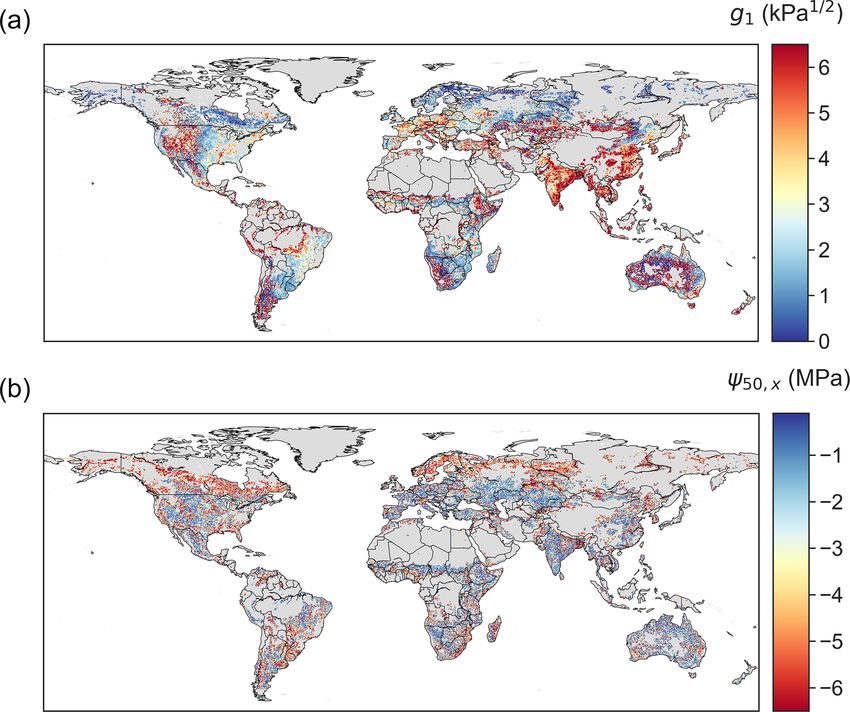
2400                                                                     Y. Liu et al.: Global pattern of plant hydraulic traits

gas exchange during drought (Matheny et al., 2017; Barros           vironmental conditions (Hochberg et al., 2018; Novick et al.,
et al., 2019). Plant hydraulic traits play critical roles in pre-   2019; Feng et al., 2019; Mrad et al., 2019). Furthermore,
dicting stomatal response to stress (Sperry et al., 2017; Liu       isohydricity is influenced by both stomatal and xylem traits
et al., 2020a), plant water storage (Huang et al., 2017), leaf      (Martínez-Vilalta et al., 2014), which do not always co-vary
desiccation (Blackman et al., 2019), and drought-driven tree        (Manzoni et al., 2013; Martínez-Vilalta et al., 2014; Bartlett
mortality risk (Anderegg et al., 2016; Powell et al., 2017; Liu     et al., 2016; Martínez-Vilalta and Garcia-Forner, 2017). Es-
et al., 2017; De Kauwe et al., 2020). As a result of their ef-      timating intrinsic xylem and stomatal traits separately is,
fect on the surface energy balance, plant hydraulic traits also     therefore, necessary for better assessment of plant drought
impact the magnitude of land–atmosphere feedbacks (An-              response.
deregg et al., 2019). In dry tropical forests, leaf water po-          From a modeling perspective, as plant hydraulics has been
tential – which is directly influenced by hydraulic traits – has    increasingly recognized as a central link connecting hydro-
also been shown to affect leaf phenology (Xu et al., 2016).         climatic processes and ecosystem ecology (Sack et al., 2016;
As a result, it has been increasingly recognized that plant hy-     McDowell et al., 2019), land surface and dynamic vegetation
draulic traits are important for mediating ecosystem drought        models that explicitly incorporate plant hydraulics are be-
response and hydroclimatic feedbacks at regional to global          coming more common (e.g., Xu et al., 2016; Christoffersen
scales (Choat et al., 2012; Anderegg, 2015; Choat et al.,           et al., 2016; Kennedy et al., 2019; De Kauwe et al., 2020;
2018; Hartmann et al., 2018).                                       Eller et al., 2020). However, explicit plant hydraulic repre-
   Understanding how plant hydraulic traits modulate large-         sentation also requires parameterization choices for the asso-
scale drought responses requires mapping these traits. At           ciated plant hydraulic traits. As discussed above, a bottom-
large scales, plant traits are often parameterized based on         up scaling of in situ measurements is likely to miss signif-
plant functional types (PFTs), such as evergreen needle-            icant fractions of the spatial variability in these parameters.
leaf forests, evergreen broadleaf forests, deciduous broadleaf      Alternatively, Liu et al. (2020a) took a top-down inversion
forests, mixed forests, shrublands, grasslands, and croplands.      approach by integrating a plant hydraulic model with ET
However, plant hydraulic traits can vary as much across             data observed at FLUXNET sites. This model–data fusion
PFTs as within them (Anderegg, 2015; Konings and Gentine,           approach identifies the most likely traits generating modeled
2017). Finding alternative ways to scale up in situ measure-        dynamics consistent with observations, thus providing effec-
ments using a bottom-up approach is challenging because             tive hydraulic traits that represent ecosystem-scale behav-
the spatial coverage of such measurements is often limited          iors. Similar model–data fusion approaches have been pre-
and biased towards temperate regions. Furthermore, plant hy-        viously applied in carbon cycle models (e.g. Wang et al.,
draulic traits are highly variable within species (Anderegg,        2009; Dietze et al., 2013; Quetin et al., 2020). Not surpris-
2015) and even between different components of a single             ingly, many of these applications suggest that integrating in-
plant and across vertical gradients within individual trees         formative observations is among the keys to effectively con-
(Johnson et al., 2016). Alternatively, because microwave re-        straining model parameters.
mote sensing observations of vegetation optical depth (VOD)            Here, we use the model–data fusion approach to evaluate
are sensitive to leaf water potential (Momen et al., 2017;          the global pattern of ecosystem-scale plant hydraulic traits.
Konings et al., 2019; Holtzman et al., 2021), they may carry        Specifically, we determined global maps of five plant hy-
implicit information that can be used to disentangle plant hy-      draulic traits (see Sect. 2). To effectively constrain the traits,
draulic traits, without the need for explicit upscaling.            we use several data sets derived from microwave remote
   Konings and Gentine (2017) first derived plant hydraulic         sensing observations, each of which is affected by plant hy-
trait variations at large scales by using VOD to calculate the      draulic behavior. Specifically, we used VOD, surface soil
effective ecosystem-scale isohydricity. The isohydricity re-        moisture, and ET estimates from a microwave implemen-
flects the response of leaf water potential as soil water poten-    tation of the Atmosphere–Land Exchange Inverse (ALEXI)
tial dries down (Tardieu and Simonneau, 1998). At a stand           framework. The resulting retrieved ecosystem-scale plant hy-
scale, this plant physiological metric has been used to explain     draulic traits are then compared to available in situ observa-
photosynthesis variations (Roman et al., 2015) and drought          tions. Having derived spatial maps of variations in plant hy-
mortality risk (McDowell et al., 2008) across species. At           draulic traits, we explore whether simple alternatives to PFTs
a global scale, remote-sensing-derived isohydricity patterns        can be built to facilitate parameterizing land surface mod-
have been used to explain photosynthesis sensitivity to va-         els. We derive several so-called hydraulic functional types
por pressure deficit and soil moisture in North American            (HFTs) based on the clustering of retrieved hydraulic traits
grasslands (Konings et al., 2017) and the Amazon (Giardina          and examine their spatial patterns.
et al., 2018), to explore the interannual variability in isohy-
dricity (Wu et al., 2020) and to explain the relationship be-
tween drought resistance and resilience in gymnosperms (Li
et al., 2020). However, because isohydricity is an emergent
rather than intrinsic property, it is subject to change with en-

Hydrol. Earth Syst. Sci., 25, 2399–2417, 2021                                        https://doi.org/10.5194/hess-25-2399-2021
Y. Liu et al.: Global pattern of plant hydraulic traits                                                                       2401

2     Methods                                                      be identified using the model–data fusion approach, even at a
                                                                   much finer scale of a flux tower footprint (Liu et al., 2020a).
2.1    Plant hydraulics model                                      The linearized form here keeps the number of parameters
                                                                   minimal.
For the model underlying the model–data fusion system,                The model assumes a single water storage pool in the
we used a soil–plant system model adapted from Liu et al.          canopy. The size of this pool is recharged by plant water up-
(2020a) that incorporates plant hydraulics. The soil is char-      take (J ) and reduced by transpiration (T ), with a vegetation
acterized by two layers, i.e., a hydraulically active rooting      capacitance parameter C determining the proportionality be-
zone extending to the maximum rooting depth, topped by a           tween that water flux and the corresponding change in plant
surface layer with a fixed depth of 5 cm. Soil moisture in both    water potential.
layers is modeled based on the soil water balance, as follows:
                                                                       dψl
   ds1                                                             C       = J −T                                               (6)
Z1     = P − L12 − E                                        (1)         dt
   dt
   ds2                                                             Transpiration is computed using the Penman–Monteith equa-
Z2     = L12 − L23 − J,                                     (2)
   dt                                                              tion.
where Z1 (= 5 cm) and Z2 are the thickness of the two soil                1 Rnl + ρa cp ga D
layers, and s1 and s2 are the volumetric soil moisture of the      T =                       ,                                (7)
                                                                         λ 1 + γ (1 + ga /gs )
two layers. P is the precipitation rate, E is the soil evapora-
tion rate, and J is plant water uptake. The L12 and L23 are        where 1 is the rate of change of saturated vapor pressure
vertical fluxes between the two soil layers and out of the root-   with air temperature, Rnl is the fraction of net radiation ab-
ing zone, respectively. Both are calculated based on Darcy’s       sorbed by the leaves, ρa is the air density, cp is the specific
law. A constant soil moisture below the rooting zone is as-        heat capacity of air, ga is the aerodynamic conductance, D is
sumed as the boundary condition for the L23 calculation. The       the vapor pressure deficit, λ is the latent heat of vaporization,
soil evaporation rate E is calculated as the potential evapo-      γ is the psychrometric constant, and gs is the stomatal con-
ration from the Penman equation multiplied by a stress fac-        ductance to water vapor per unit ground area. The stomatal
tor of s1 /n, where n is the soil porosity. The potential evap-    conductance is calculated using the Medlyn stomatal conduc-
oration is driven by the fraction of total net radiation that      tance model (Medlyn et al., 2011), while omitting cuticular
penetrates through the canopy to the ground surface based          and epidermal losses by assuming zero minimum stomatal
on Beer’s law (Campbell and Norman, 1998). The remain-             conductance.
ing fraction of total net radiation is absorbed by the leaves
and drives transpiration (Eq. 7). Plant water uptake J is de-                           g1      A
                                                                   gs = a0 LAI 1 + √               ,                             (8)
termined as the product of the whole-plant conductance (gp )                             D      ca
and the water potential gradient between the soil (ψs ) and the
                                                                   where a0 = 1.6 is the relative diffusivity of water vapor with
leaf (ψl ), as follows:
                                                                   respect to CO2 , LAI is the leaf area index, and g1 is the
J = gp (ψs − ψl ),                                          (3)    slope parameter, inversely proportional to the square root of
                                                                   marginal water use efficiency (Medlyn et al., 2011; Lin et al.,
where the soil water potential is calculated from s2 based on      2015). A is the biochemical demand for CO2 calculated us-
the empirical soil water retention curve by Clapp and Horn-        ing the photosynthesis model (Farquhar et al., 1980), and ca
berger (1978).                                                     is the atmospheric CO2 concentration. Photosynthesis is lim-
                                                                   ited by either ribulose-1, 5-bisphosphate (RuBP) regenera-
ψs = ψs,sat (s2 /n)−b0 .                                    (4)
                                                                   tion or by the carboxylation rate. Water stress is assumed
Above, ψs,sat is the saturated soil water potential, n is the      to restrict photosynthesis under the carboxylation-limited
soil porosity, and b0 is the shape parameter. Plant water up-      regime through a down-regulated maximum carboxylation
take from the thin surface layer is assumed to be negligible.      rate (Vcmax ), following Kennedy et al. (2019) and Fisher et al.
The whole-plant conductance varies with leaf water poten-          (2019).
tial, following a linear vulnerability curve as follows:
                                                                                       ψl
                                                                 Vcmax = 1 −                Vcmax,w ,                        (9)
                      ψl                                                            2 ψ50,s
gp = gp,max 1 −               ,                           (5)
                    2 ψ50,x
                                                                   where ψ50,s is the leaf water potential when Vcmax drops
where gp,max is the maximum xylem conductance, and ψ50,x           to half of its maximum value under well-watered conditions
is the water potential at which xylem conductance drops to         (Vcmax,w ).
half of its maximum. A linear vulnerability curve is used be-         The model was driven by climate conditions at a 3 h scale.
cause the nonlinearity of the vulnerability curve can hardly       To temporally integrate the model, a forward Euler method

https://doi.org/10.5194/hess-25-2399-2021                                       Hydrol. Earth Syst. Sci., 25, 2399–2417, 2021
2402                                                                  Y. Liu et al.: Global pattern of plant hydraulic traits

was used for computational efficiency, except for the calcu-     where a and b are the scaling parameters from LAI to βAGB,
lation of plant water uptake, for which Eqs. (2) through (6)     and c is the linearized slope of the pressure–volume curve.
were linearized at each time step and then solved analytically   The a, b, and c parameters vary across pixels and were
to ensure numerical stability. The modeled time series of ET     retrieved as additional inversion parameters as part of the
(E +T ), surface soil moisture (s1 ), and VOD were compared      model–data fusion process.
with the microwave remote sensing observations as described
below.                                                           2.2.2   Soil moisture

2.2     Microwave remote sensing constraints                     We also used the associated surface soil moisture retrievals
                                                                 from the LPRM as additional constraints. Instead of perform-
To derive plant hydraulic traits, the model in Sect. 2.1 was     ing a direct comparison between modeled and retrieved soil
constrained by microwave remote sensing products of VOD          moisture, we followed the widely used approach of assimi-
and surface soil moisture, as well as by remote-sensing-         lating retrieved soil moisture only after matching its cumula-
derived ET, all with a spatial resolution of 0.25◦ .             tive distribution function (cdf) to the modeled soil moisture
                                                                 (Reichle and Koster, 2004; Su et al., 2013; Parrens et al.,
2.2.1    VOD                                                     2014). Because the magnitudes of both retrieved and mod-
                                                                 eled soil moisture are highly dependent on the retrieval al-
We used VOD and surface soil moisture derived from the
                                                                 gorithm and specific model structure (Koster et al., 2009),
Japan Aerospace Exploration Agency (JAXA) Advanced Mi-
                                                                 this cdf-matching approach reduces the effect of bias in ei-
crowave Scanning Radiometer for Earth Observing System
                                                                 ther the model or observations on the ability of the soil mois-
(EOS; collectively AMSR-E) retrieved by the land param-
                                                                 ture observations to act as useful constraints. Unlike VOD,
eter retrieval model (LPRM; Owe et al., 2008; Vrije Uni-
                                                                 surface soil moisture does not have a strong diurnal cycle.
versiteit Amsterdam and NASA GSFC, 2016). This data set
                                                                 Additionally, because the canopy and soil often reach ther-
is based on observations at X-band frequency (10.7 GHz),
                                                                 mal equilibrium at night, AMSR-E retrievals at 13:30 have
which is primarily sensitive to the water content of the up-
                                                                 greater retrieval errors than at 01:30 (Parinussa et al., 2016).
per canopy layers (Frappart et al., 2020). Here, we used an
                                                                 Therefore, only 01:30 surface soil moisture was included as
X-band record rather than lower microwave frequencies to
                                                                 a model constraint here.
reduce errors associated with potential sensitivities of these
lower frequencies to xylem water potential, which might de-      2.2.3   Evapotranspiration
viate from leaf water potential. Data for 2003–2011 were
used. Outliers that are more than three scaled median abso-      The model was also constrained by weekly ET during
lute deviations away from the median were filtered out and       2003–2011. ET was estimated using the Atmosphere–Land
attributed to high-frequency noise in the retrievals common      Exchange Inverse (ALEXI) algorithm (Anderson et al.,
to VOD data sets (Konings et al., 2015, 2016). A 5 d moving      1997, 2007; Holmes et al., 2018). Most remote-sensing-
average method was applied to midday and midnight VOD,           based ET data sets assume prior values of stomatal parame-
respectively, to further diminish noise in the raw data. Both    ters (Kalma et al., 2008; Wang and Dickinson, 2012), which
ascending (01:30 local time – LT) and descending (13:30 LT)      would make it circular to retrieve plant traits based on these
observations were used, to enable them to constrain subdaily     data sets. By contrast, the ALEXI framework is relatively
variations in plant hydraulic dynamics.                          independent of prior assumptions on vegetation properties.
   To relate VOD and leaf water potential, we noted that         To achieve this independence, ALEXI uses a two-source en-
VOD is proportional to vegetation water content (VWC).           ergy balance method and is constrained to be consistent with
In turn, VWC is determined by the product of aboveground         the boundary layer evolution (Anderson et al., 2007; Holmes
biomass (AGB) and plant relative water content (RWC).            et al., 2018). We further used a version of ALEXI based on
                                                                 microwave-derived land surface temperatures rather than op-
VOD = βVWC = β AGB × RWC,                                (10)
                                                                 tical ones as in the classic ALEXI implementations. When
where β is the scaling parameter depending on the structure      compared to in situ observations, microwave–ALEXI and
and dielectric properties of plants (Kirdiashev et al., 1979).   optical–ALEXI performed similarly (Holmes et al., 2018),
As in Momen et al. (2017), AGB is represented using lin-         but the microwave-based version has the advantage of hav-
earized relationships of LAI and ψl respectively. The rela-      ing more observations because, unlike optically derived esti-
tionship between RWC and ψl usually follows a Weibull            mates, it is not limited by cloud cover. The 0.25◦ resolution of
pressure–volume curve. However, it has been successfully         the microwave–ALEXI product is also more consistent with
linearized in previous theoretical and observational applica-    the other components of our model–data fusion system.
tions (Manzoni et al., 2014; Momen et al., 2017; Konings and
Gentine, 2017). Thus, VOD is modeled as follows:
VOD = (a + b LAI) (1 + c ψl ),                           (11)

Hydrol. Earth Syst. Sci., 25, 2399–2417, 2021                                     https://doi.org/10.5194/hess-25-2399-2021
Y. Liu et al.: Global pattern of plant hydraulic traits                                                                                       2403

2.3   Model–data fusion                                              VOD, surface soil moisture, and ET with the three categories
                                                                     of observations. Observations on rainy (daily cumulative pre-
Plant hydraulic traits and several other model parameters            cipitation > 1 cm) or freezing (daily minimum air tempera-
controlling plant hydraulic behavior were retrieved using a          ture < 0 ◦ C) days were removed. Each of the remaining ob-
Markov chain Monte Carlo (MCMC) method, which deter-                 servations was considered independent, following a Gaus-
mined the parameter values that yield model output most              sian distribution with a mean of the modeled value and the
consistent with observed constraints. A total of 13 parame-          standard deviation of the corresponding category (i.e., one of
ters were retrieved, including five plant hydraulic traits (g1 ,     σVOD , σSM , and σET ). The likelihood of all observations were
ψ50,s , C, gp,max , and ψ50,x ), three scaling parameters relating   then combined after reweighting each constraint based on its
VOD to ψl (a, b, and c in Eq. 11), two soil properties (includ-      number of observations. That is, in the following:
ing b0 in Eq. 4 and the subsurface boundary condition of soil
moisture in the deepest layer), and three uncertainty values,        log(L(yv(1:nv ) , ye(1:ne ) , ys(1:ns ) | θ )
describing the standard deviation of the observational noise                X
                                                                              1 nv                                 1 X ne
of VOD (σVOD ), surface soil moisture (σSM ), and ET (σET ),             =              log L(yv(i) | θ ) +               log L ye(i) | θ
respectively. An adaptive metropolized independence sam-                     nv i=0                                ne i=0
pler was used to generate posterior samples (Ji and Schmi-                      n s

                                                                           1 X                                nv + ne + ns
dler, 2013). This sampling method was designed to facilitate            +            log L(ys(i) | θ )                       ,                (13)
                                                                           ns i=0                                    3
convergence especially for nonlinear models and has been
shown to be effective for retrieving plant hydraulic traits at       where L is likelihood of observed VOD (yv ), ET (ye ), and
flux tower sites (Liu et al., 2020a). To reduce the dimension-       surface soil moisture (ys ) under given parameters θ (includ-
ality of the parameter space and facilitate convergence, the         ing all the 13 parameters to be retrieved). nv , ne , and ns
MCMC jointly sampled all parameters, except the three scal-          are the number of valid data of VOD, ET and surface soil
ing parameters of VOD. For these parameters, the optimal             moisture, respectively. Due to the unbalanced number of ob-
values were determined conditional on the rest of the param-         servations among the measurement types, renormalizing the
eters after each sampling step based on least squared error.         weights in each category based on its number of observa-
That is, after each sampling step, the three values were opti-       tions avoids overweighting of semidaily VOD and surface
mized so as to minimize the least-squares difference between         soil moisture over weekly ET observations.
observed VOD and the predicted VOD conditional on simu-                  For the global retrievals, pixels classified by MODIS land
lated ψl and the optimized parameter values for a, b, and c.         cover data as wetland, urban area, barren area, snow/ice cov-
   The MCMC also incorporated prior information about pa-            ered, or tundra dominated were excluded from the analysis.
rameter ranges and constraints on their realistic combina-           Pixels for which VOD is below 0.15 or above 0.8 were also
tions. For ψ50,x , a generalized extreme value distribution was      excluded to remove sparsely vegetated pixels and extremely
used as the prior for the corresponding PFT. The distribution        dense vegetation areas, respectively. The most densely vege-
was fitted using measurements of species belonging to each           tated areas were removed because low microwave transmis-
PFT in the TRY database (Kattge et al., 2011). The corre-            sivity significantly reduces the accuracy of VOD and soil
sponding PFT of each species was determined based on the             moisture retrievals there (Kumar et al., 2020), and low VOD
PLANTS database (USDA, NRCS, 2020) and the Encyclo-                  pixels were removed to reduce inaccuracies due to ground
pedia of Life (Parr et al., 2014). For PFTs not included in          volume scattering and low vegetation density. For the re-
the TRY database, a distribution fitted using measurements           maining pixels, parameters were retrieved using observa-
for all species was used as the prior (Fig. S1). We also incor-      tions in 2004 and 2005, during which the El Niño event
porated a physiological constraint from meta-analysis sug-           and the elevated tropical North Atlantic sea surface tem-
gesting stomatal conductance is downregulated before sub-            peratures induced drought stress in many regions across the
stantial xylem embolism occurs (Martin-StPaul et al., 2017;          globe (Phillips et al., 2009; FAO, 2014). Here, we used only
Anderegg et al., 2017), as follows:                                  2 years of observations, rather than the entire period, to re-
                                                                     duce the computational load of model–data fusion. The re-
|ψ50,s | < |ψ50,x |.                                         (12)
                                                                     maining 7 years were used for testing. Separating retrieval
The physiological constraint, which was also used in Liu             and testing periods also helped to (potentially) identify over-
et al. (2020a), avoids unrealistic combinations of parame-           fitting.
ters that nevertheless match the data. For other parameters,             For each pixel, four MCMC chains were used. Each started
uniform noninformative priors spanning realistic ranges were         randomly within the prior parameter ranges, and each gener-
used (Table S1).                                                     ated 50 000 samples. Within- and among-chain convergences
   The cost function in the MCMC (i.e., the reverse of the           were diagnosed by Gelman–Rubin (< 1.2) and Geweke val-
likelihood function multiplied by the prior) determines the          ues (< 0.2; Brooks and Gelman, 1998). Across the studied
estimated posterior distribution of parameters. The likeli-          pixels, all parameters converged for 79 % of pixels, while
hood function was calculated by comparing the modeled                at least half of the parameters converged for 97 % of pix-

https://doi.org/10.5194/hess-25-2399-2021                                            Hydrol. Earth Syst. Sci., 25, 2399–2417, 2021
2404 Y. Liu et al.: Global pattern of plant hydraulic traits
els. The remaining 3 % of pixels that did not converge were values of VOD, surface soil moisture, and ET. The prescribed
removed from the analysis. For each pixel, 200 samples were standard deviations of noise in VOD, surface soil moisture„
randomly selected from the chains after step 40 000 as pos- and ET, i.e., 0.05, 0.08, and 0.5 mm d−1 , respectively, were
terior samples of parameters. Ensemble means of VOD, sur- chosen to be within the mid-50 % ranges retrieved using real
face soil moisture, and ET modeled using posterior samples data. The parameters retrieved using the model–data fusion
were compared to observations during the period 2003–2011. approach were then compared with the prescribed values.
Posterior means of the hydraulic traits in each pixel were
used for analysis below. 2.5.2 Comparison between derived traits and in situ
measurements
2.4 Climate forcing and ancillary properties
Because hydraulic traits are often measured at a single plant
The model–data fusion system was run at 0.25◦ resolution. or a segment scale that is much smaller than the ecosystem
Meteorological drivers at this spatial resolution and the 3 h scale used in model–data fusion, and because of the rela-
temporal resolution used by the model were derived from tively coarse spatial resolution of the remote sensing data
the Global Land Data Assimilation System (GLDAS; Rodell used as constraints here, a one-to-one comparison between
et al., 2004; Beaudoing and Rodell, 2020). In particular, in situ data and model–data-fusion-derived values is likely to
GLDAS-derived forcings include net shortwave radiation, be dominated by representativeness error. Instead, we aggre-
air temperature, precipitation, surface atmospheric pressure, gated both in situ measurements and the traits derived here
specific humidity, and aerodynamic conductance calculated by PFTs to evaluate whether across-PFT patterns can be cap-
using the ratio between the sensible heat net flux and the dif- tured. Among the most ecologically important and widely
ference between air and surface skin temperatures. LAI data measured traits are g1 and ψ50,x , which indicate stomatal
from the MODIS (Moderate Resolution Imaging Spectrora- marginal water use efficiency and vulnerability to xylem cav-
diometer) product MCD15A3H v006 (Myneni et al., 2015), itation, respectively. Synthesized data sets of g1 from Lin
with a 500 m resolution, were aggregated to a 0.25◦ scale, us- et al. (2015) and ψ50,x from Kattge et al. (2011), based on
ing a Google Earth Engine, to be consistent with the GLDAS in situ measurements covering a variety of species and cli-
climatic drivers. Missing data were linearly interpolated, and mate types, were used for comparison. In addition, Trugman
a Savitzky–Golay filter (Savitzky and Golay, 1964) was ap- et al. (2020) derived a map of tree ψ50,x across the con-
plied to diminish high-frequency noise in the LAI time series. tinental United States at a 1◦ resolution, which integrated
To estimate Vcmax,w , a PFT map from the GLDAS land cover measurements in the Xylem Functional Traits Database and
map derived from MODIS was used (Fig. S2). The Vcmax,w the US Forest Service Forest Inventory and Analysis (FIA)
of each PFT was set as the static PFT-average from Walker long-term permanent plot network. This map was used for
et al. (2017) and corrected by temperature, following Med- a pixel-wise comparison with the ψ50,x retrieved here in US
lyn et al. (2002). The maximum rooting depth was obtained areas dominated by forests. To perform this comparison, our
from a global map synthesized from in situ observations (Fan model–data-fusion-derived traits were first aggregated from
et al., 2017). Soil texture from the Harmonized World Soil 0.25◦ to the 1◦ resolution of the estimates by Trugman et al.
Database (FAO/IIASA/ISRIC/ISSCAS/JRC, 2012) was used (2020).
to calculate soil drainage parameters based on empirical re-
lations (Clapp and Hornberger, 1978). 2.5.3 Clustering analysis
2.5 Analyses To understand the global pattern of retrieved plant hydraulic
traits, we constructed hydraulic functional types (HFTs) us-
2.5.1 Observing system simulation experiment ing the K-means clustering method (MacQueen, 1967). This
method classifies each pixel to the nearest mean, i.e., the
To test the capability of the model–data fusion approach to cluster center in the five-dimensional space spanned by the
correctly retrieve parameters under the presence of observa- modeled hydraulic traits. To find the optimal number of clus-
tional noise, we conducted an observing system simulation ters, we calculated the ratio between the variance within clus-
experiment (OSSE) for 50 pixels. The 50 pixels were ran- ter traits across three to 20 clusters. The elbow method was
domly distributed across the globe. The OSSE uses synthetic used to derive the optimal number of clusters (Kodinariya
rather than real observations to test data assimilation uncer- and Makwana, 2013). That is, the optimal number of clus-
tainty, among other objectives (Arnold and Dey, 1986; Near- ters was chosen based on the inflection point (elbow) of the
ing et al., 2012; Errico et al., 2013). At each pixel, the time curve relating the above ratio and the number of clusters.
series of VOD, surface soil moisture, and ET were generated The global pattern of these HFTs were examined. To pro-
by using the model (Sect. 2.1) with prescribed parameters. vide insight into whether HFTs could be used as an alter-
To mimic the presence of observational noise in real observa- native to PFTs, we evaluated how much the accuracy of es-
tional estimates, white noise was then added to the simulated timated VOD and ET would degrade if VOD and ET were
Hydrol. Earth Syst. Sci., 25, 2399–2417, 2021 https://doi.org/10.5194/hess-25-2399-2021Y. Liu et al.: Global pattern of plant hydraulic traits 2405
modeled using hydraulic traits based on an HFT-based clus- atively lower in central Australia, southern South America,
tering rather than a more typical PFT-based clustering. That and the southwestern US, where highly heterogeneous vege-
is, we calculated the simulated VOD and ET by assigning hy- tation cover such as savannas and coexisting grass and shrubs
draulic traits as the center values for the HFT present at each within a pixel could undermine model accuracy. The median
pixel, rather than by using the average derived value across and mid-50 % range of surface soil moisture R 2 is 0.22 and
each PFT as the PFT-wide value. Several factors differ be- (0.08,0.42), respectively. Modeled surface soil moisture is
tween this calculation and the potential reduced error from less accurate in croplands (likely due to irrigation) and in
using HFTs in land surface models. For example, land sur- boreal regions, eastern China, Europe, and the mid-western
face models often use subgrid-scale tiling systems that are and eastern US. These regions largely overlap with those
more complex than the pixel-scale calculations performed where the observed soil moisture from AMSR-E is weakly
here. The calculation here also did not account for uncertain- correlated with the reanalysis product of ERA-Interim that
ties in determining the optimal PFT-wide or HFT-wide values integrates ground observations (Parinussa et al., 2015), sug-
or, indeed, the mapping of PFTs or HFTs to begin with (Poul- gesting greater uncertainties of surface soil moisture from
ter et al., 2011; Hartley et al., 2017). Nevertheless, this analy- AMSR-E compared to other regions. The overall accuracy
sis provides first-order insight into the capacity of HFT-based of estimated VOD, ET, and surface soil moisture both within
parameterization to improve over a PFT-based approach. (Fig. S3) and outside (Fig. 2) the training period 2004–2005
suggest that the model and the derived traits effectively rep-
resent plant hydraulic dynamics.
3 Results
3.3 Global pattern of plant hydraulic traits
3.1 Parameter retrieval in the OSSE
The retrieved stomatal conductance slope parameter g1 ,
Across the 50 pixels tested in the OSSE, the prescribed traits which is inversely proportional to marginal water use effi-
can be recovered using model–data fusion, with high Pear- ciency (Eq. 6), exhibits clear spatial patterns (Fig. 3a). High
son correlations between the assumed and retrieved values g1 values arise in areas covered by grasses and savannas,
(Fig. 1). The hydraulic traits of g1 , ψ50,x , and gp,max , along such as the western US, the Sahel, central Asia, northern
with the soil parameters (b0 in Eq. 4 and the boundary condi- Mongolia, and inner Australia. This pattern is consistent with
tion bc ), are accurately recovered (r ≥ 0.77). The C and the predictions from experimental data and optimality theory
ratio between ψ50,s and ψ50,x showed larger discrepancies that herbaceous species – given the low cost of stem wood
and greater uncertainty ranges due to the presence of (sim- construction per unit water transport – should have the largest
ulated) observational noise. For all parameters, the residual g1 , i.e., be the least water-use efficient (Manzoni et al., 2011;
errors are randomly distributed rather than scaling the true Lin et al., 2015). In addition, croplands in India and east-
parameter value. Overall, the OSSE supports the effective- ern China also show high g1 , consistent with the high isohy-
ness of the model–data fusion approach. dricity of these regions (Konings and Gentine, 2017). Con-
sistent with ground measurements that suggest g1 increases
3.2 Accuracy of modeled VOD, ET, and surface soil
with biome average temperature (Lin et al., 2015), the g1 de-
moisture
rived here is also (on average) lower in boreal ecosystems
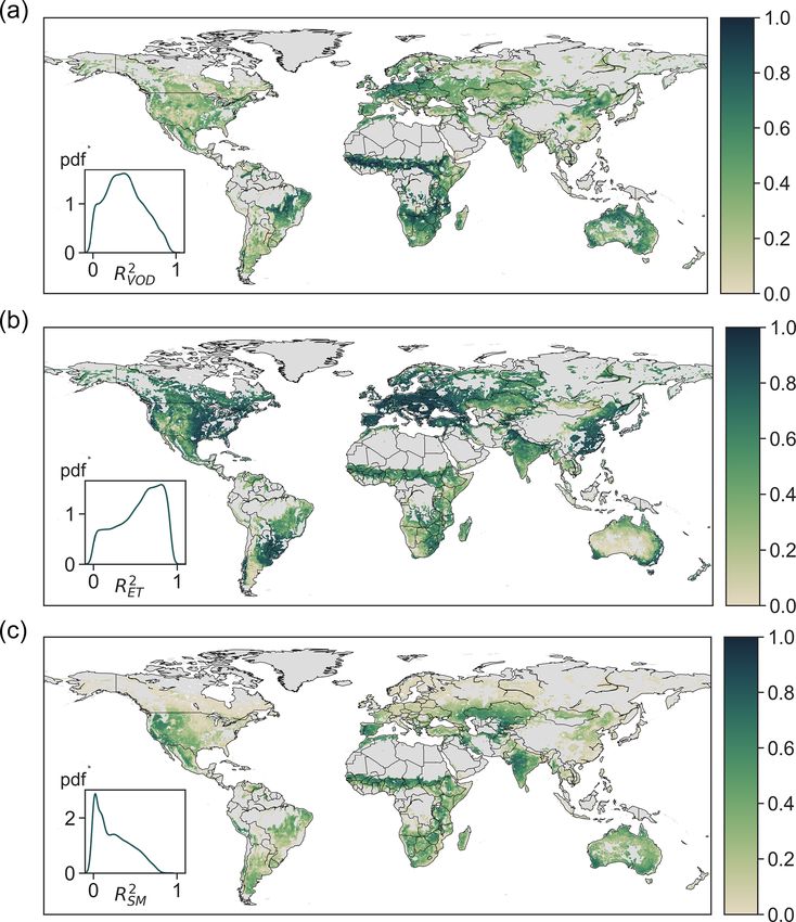
Over the entire study period of 2003–2011, the coefficient than in temperate and tropical ecosystems.
of determination (R 2 ) between estimated and observed VOD Highly negative ψ50,x values are found in boreal evergreen
has a median of 0.38 and a mid-50 % range of (0.22,0.55) needleleaf forests and in arid or seasonally dry biomes cov-
across the globe (Fig. 2a). The estimated VOD is highly cor- ered by forests, shrubs or savannas, such as the western US,
related with observations in northern and southwestern Aus- central America, eastern south America, southeastern Africa,
tralia, northeastern China, India, central Europe, Africa, and and Australia (Fig. 3b). However, ψ50,x is more spatially
eastern South America. The high VOD accuracy in these scattered than g1 . This could partially arise from the greater
areas is likely partially a result of the large contribution coefficient of variation across ensembles of ψ50,x (Fig. 4),
of biomass to VOD due to strong biomass seasonality in suggesting ψ50,x is less tightly constrained compared to g1
these areas (Liu et al., 2011; Momen et al., 2017). Notably, (consistent with site-scale model–data fusion efforts in Liu
however, even in areas where VOD has been shown to be et al. (2020a) and the uncertainty estimates in the OSSE;
less correlated with LAI, including central Australia, central Fig. 1). This additional uncertainty might translate to more
Asia, southern Africa, and the western US (Momen et al., noise in the ensemble medians for ψ50,x than that for g1 .
2017), the estimated VOD accounting for the signature of Maps of other hydraulic traits are shown in Fig. S4. The
leaf water potential is also able to capture observed VOD. patterns of hydraulic traits exhibit greater variability beyond
The model also accurately estimates observed ET with a me- PFT distribution (Fig. S2) and only limited correlation with
dian R 2 of 0.60 and a mid-50 % range of (0.36,0.78; Fig. 2b). soil and climate conditions (Fig. S5).
Unlike in the majority of the world, the R 2 of ET is rel-
https://doi.org/10.5194/hess-25-2399-2021 Hydrol. Earth Syst. Sci., 25, 2399–2417, 20212406 Y. Liu et al.: Global pattern of plant hydraulic traits
Figure 1. Comparison between the prescribed and retrieved plant hydraulic traits (g1 , ψ50,s /ψ50,x , ψ50,x , gp,max , and C) and soil properties
(b0 and bc ) in the observing system simulation experiment. The black dots and gray lines represent the mean and range of 1 standard deviation
of the retrieved posterior distributions. The diagonal dashed line is the 1 : 1 line. Pearson correlation coefficient (r) between the prescribed
and retrieved parameters is noted.
Among the plant hydraulic traits, we found strong coor- mate, and due to the uncertainty in the kriging-based inter-
dination between the vulnerability of stomata and the xylem polation used for upscaling from the sparse FIA plots to each
(ψ50,s and ψ50,x ) across space (Fig. S5), consistent with ex- 1◦ pixel. Nevertheless, this discrepancy highlights the scale
isting evidence from ground measurements (Anderegg et al., gap between traits measured for a single plant and those de-
2017). Other hydraulic traits are only weakly correlated, in- rived for an ecosystem.
cluding gp,max and ψ50,x (Fig. S5), which is consistent with
the previous finding suggesting the safety–efficiency trade- 3.4 Hydraulic functional types (HFTs)
off of xylem traits is weak across > 400 species (Gleason
et al., 2016).
Across PFTs, evergreen needleleaf forests have the low- We built six HFTs (termed H1 to H6) using the K-means
est g1 , followed by deciduous broadleaf forests and shrub- clustering method. The number of clusters (six) was chosen,
lands (Fig. 5a). Grasslands and croplands have the highest using the elbow method, based on the inflection point of the
g1 . This trend follows the across-PFT pattern found by Lin ratio of within- to across-cluster variance (Fig. S6). Across
et al. (2015). The estimated across-PFT pattern of mean ψ50,x the six HFTs, the across-cluster variance is 1.7 times as large
is also consistent with measurements included in the TRY as the within-cluster variance. The HFTs explain 57 % of the
database (Kattge et al., 2011), i.e., lowest in grasslands and total variance in hydraulic traits across the globe. The cluster
highest in evergreen needleleaf forests (Fig. 5b). However, centers of the six HFTs are characterized by distinct com-
across the globe, we found that the average standard devi- binations of hydraulic traits (Fig. 7a). Specifically, H1 and
ation within PFTs is 3.6 and 2.3 times the standard devia- H2 feature low ψ50,s and ψ50,x and are mainly distributed
tion across PFTs for g1 and ψ50,x , respectively. The large in boreal forest and arid or seasonally dry biomes, includ-
within-PFT variation is consistent with in situ observations ing the western US, central America, southeastern Africa,
(Anderegg, 2015), indicating that PFTs are not informative central Asia, and Australia (Fig. 7b). H3 and H4 are char-
of plant hydraulic traits. acterized by low and high vegetation capacitance (C), re-
We further compared the retrieved ψ50,x for specific loca- spectively, though both have low gp,max . H3 is mainly but
tions to an alternative estimate upscaled from Forest Inven- not exclusively distributed in grasslands and savannas in the
tory and Analysis (FIA) surveys (Fig. 6). Consistent with the central US, the Nordeste region in Brazil, eastern and south-
FIA-based estimate, the retrieved ψ50,x are overall lower in ern Africa, and eastern Australia, as well as in the Miombo
pixels dominated by evergreen needleleaf forests than in ev- woodlands. H4 is distributed in shrublands in the southwest-
ergreen and deciduous broadleaf forests and mixed forests. ern US, Argentina, southern Africa, northwestern India, and
However, across pixels, the ecosystem-scale ψ50,x derived northeastern Australia. H5, often found in tropical and sub-
from remote sensing vary significantly more than the esti- tropical regions, is characterized by large gp,max and capac-
mates from the Trugman et al. (2020) data set. Some fraction itance. H6 is characterized primarily by high g1 , which in-
of this discrepancy might be due to intra-species variability cludes croplands in India, southeastern Asia, and central and
in ψ50,x , which is not accounted for in the FIA-based esti- eastern China. Note that the pattern of HFTs (Fig. 7b) is sub-
stantially distinct from the distribution of PFTs (Fig. S2), il-
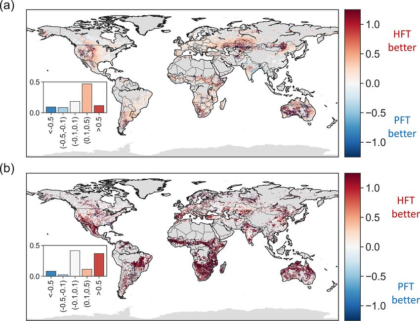
Hydrol. Earth Syst. Sci., 25, 2399–2417, 2021 https://doi.org/10.5194/hess-25-2399-2021Y. Liu et al.: Global pattern of plant hydraulic traits 2407 Figure 2. Assimilation accuracy (R 2 ) of (a) VOD, (b) ET, and (c) soil moisture during the entire study period (2003–2011). Insets show the probability distribution (pdf) of R 2 across the entire study area. The gray shaded area is not included in analysis. lustrating the limitations of parameterizing plant hydraulics of ET increases by more than 0.1 in 58 % of the analyzed based on PFTs. area (Fig. 8a). ET is mainly improved in arid or season- Using averaged traits per PFT, instead of pixel-specific ally dry biomes, including the western US, southern South traits to calculate VOD and ET, led to a median increase America, southern and eastern Africa, central Asia, and Aus- in normalized root mean square error (nRMSE, with the tralia. In addition, the nRMSE of VOD is also improved long-term average used for normalization) of 0.82 and 0.58, by more than 0.5 in 37 % of the analyzed area using HFTs respectively. This degradation of accuracy is unsurprising rather than PFTs (Fig. 8b). Areas exhibiting reduced error given the high spatial variability in hydraulic traits and the are mainly located in the southwestern US, central Amer- fact that PFTs are not categorized specifically to distinguish ica, eastern South America, the Mediterranean, Africa, and plant hydraulic functions. However, using the hydraulic traits Australia, where variation in leaf water potential has a strong averaged per HFT instead improves prediction accuracy over signature on VOD (Momen et al., 2017). These findings sug- the PFT-based predictions. When compared to using pixel- gest the importance of the appropriate parameterization of specific values, using average traits based on HFTs increases hydraulic traits on capturing leaf water potential and ET vari- the nRMSE by 0.65 and 0.42 for VOD and ET, respectively. ations at an ecosystem scale. In each case, this is less than the degradation when PFT- based averages are used. Indeed, when PFT-based instead of HFT-based model estimates are compared, the nRMSE https://doi.org/10.5194/hess-25-2399-2021 Hydrol. Earth Syst. Sci., 25, 2399–2417, 2021
2408                                                                         Y. Liu et al.: Global pattern of plant hydraulic traits

Figure 3. Global maps of (a) g1 and (b) ψ50,x retrieved using model–data fusion. The posterior mean of each pixel is plotted.

                                                                        drydowns (Feldman et al., 2018; Zhang et al., 2019; Feld-
                                                                        man et al., 2020) highlight the sensitivity of VOD to rela-
                                                                        tive water content. At seasonal and interannual scales, VOD
                                                                        has also been found to be modulated by leaf water poten-
                                                                        tial or relative water content, thus deviating from biomass
                                                                        signals (Momen et al., 2017; Tian et al., 2018; Tong et al.,
                                                                        2019). Here, after parsing out the impact of biomass through
                                                                        LAI, VOD provides information about leaf water potential
                                                                        variation and, therefore, contributes to constraining the un-
                                                                        derlying hydraulic traits. Kumar et al. (2020) previously as-
Figure 4. Empirical distribution across pixels of the coefficient of    similated VOD into a land surface model as a constraint on
variation (CV) of g1 and ψ50,x calculated across ensembles.             biomass, which led to improvements in modeled ET. Our
                                                                        findings suggest that, when assimilated into models with an
                                                                        explicit representation of plant hydraulics, VOD can act to
                                                                        constrain both water and carbon dynamics and their respec-
4     Discussion
                                                                        tive climatic responses. Although not explored in detail in
4.1    Contribution of VOD to informing plant hydraulic                 this study, note also that, by determining optimal values for
       behavior                                                         a, b, and c (the parameters relating VOD to ψl in Eq. 11),
                                                                        the model–data fusion system introduced here also allows the
The fact that VOD varies with plant water content allows the            determination of ψl from VOD, which may be of interest for
investigation of plant physiological dynamics at large scales.          a variety of studies of plant responses to drought. However,
Although VOD has often been used as a proxy of above-                   additional research is needed to understand the effect of the
ground biomass (e.g., Liu et al., 2015; Tian et al., 2017;              choice of retrieval algorithm and specific VOD product (Li
Brandt et al., 2018; Teubner et al., 2019), it is in fact deter-        et al., 2021) on any inferred VOD–ψl relationships. For this
mined by both biomass and plant water status (Konings et al.,           reason, any such efforts would also benefit from explicit un-
2019). VOD variations within a day (Konings and Gentine,                certainty quantification.
2017; Li et al., 2017; Anderegg et al., 2018) and during soil

Hydrol. Earth Syst. Sci., 25, 2399–2417, 2021                                             https://doi.org/10.5194/hess-25-2399-2021
Y. Liu et al.: Global pattern of plant hydraulic traits 2409
(Fig. 4). This could result from trade-offs among hydraulic
traits and the lack of constraints on the scaling from leaf wa-
ter potential to VOD, which varies across space. More prior
information about these two factors will likely contribute
to improved retrieval of plant hydraulic traits. Additionally,
the use of solar-induced fluorescence or other constraints on
photosynthesis may allow for independent information about
stomatal closure that could be used to improve the accuracy
and certainty of the retrieved hydraulic traits. However, care
should be taken that the uncertainty introduced by coupling
to a photosynthesis model does not outweigh the added ad-
vantage of this additional constraint.
4.2 Bridging the spatial scale gap of hydraulic traits
Plant hydraulic traits vary among segments from root to
Figure 5. Retrieved (a) g1 and (b) ψ50,x using model–data fusion shoot even for a single tree, causing the hydraulic sensi-
(light colored bars), grouped by PFTs, in comparison with values tivity at a whole-tree scale to be distinct from that mea-
derived from in situ measurements (dark colored bars) reported in sured at a segment scale (Johnson et al., 2016). Similarly,
Lin et al. (2015) and the TRY database (Kattge et al., 2011). Com- species diversity, canopy structure, and demographic com-
pared PFTs include evergreen needleleaf forest (ENF), deciduous position can cause large variability in hydraulic traits. As a
broadleaf forest (DBF), evergreen broadleaf forest (EBF), shrub- result, a community-weighted average of a trait may not well
land (SHB), grassland (GRA), and cropland (CRO). Bars represent represent the integrated hydraulic behavior at an ecosystem
medians of each PFT, and black lines indicate the 25th–75th per- scale, as evidenced, for example, by the significant effect of
centile ranges. The g1 averaged across gymnosperm trees and an- plant hydraulic diversity on evapotranspiration responses to
giosperm trees from Lin et al. (2015) were compared to retrieved g1
drought (Anderegg et al., 2018). Here, we also found a sub-
in pixels dominated by ENF and DBF, respectively.
stantial discrepancy between community-weighted ψ50,x and
the ecosystem-scaled value derived from representing the
property of the entire pixel, even in the most extensively sur-
veyed pixels available (biggest dots in Fig. 6). This highlights
the challenge of scaling up ground measurements of plant
hydraulic traits to a scale relevant to land surface modeling
from the bottom up. The model–data fusion used here pro-
vides an approach to help address this challenge. However,
further study is needed to explore how stand and ecosystem
characteristics shape the ecosystem-scale hydraulic traits, as
well as the effective relationship between leaf water potential
and remote-sensing-scale water content.
Figure 6. Aggregated ψ50,x from upscaling the Forest Inventory 4.3 Implications for land surface models
and Analysis (FIA) plots, based on Trugman et al. (2020), and ψ50,x
retrieved here for corresponding pixels. The point size is scaled by Because they are able to predict ET and VOD better than
number of plots used in aggregation for each pixel. PFTs (Fig. 8), the HFTs point to the potential for a better
parameterization scheme of plant hydraulics in land surface
models. Because HFTs require fewer clusters than PFTs do
Our previous study (Liu et al., 2020a) at the stand scale to model ET with the same or better accuracy, parameterizing
has shown that stomatal traits are well constrained using ET plant hydraulics by HFTs in land surface models may con-
alone, whereas xylem traits, including ψ50,x , remain largely tribute to higher model accuracy. However, because the mag-
under-constrained, in part due to lack of information on leaf nitude of state variables may differ between models, even
water potential. Incorporating VOD among the constraints as their temporal dynamics do not (Koster et al., 2009), in-
here contributes to the separation of xylem and stomatal be- cluding between a given land surface model and the model
havior. As a result, the model–data fusion approach here is, used here, using the exact values derived here may cause
to our knowledge, the first to be able to retrieve both stomatal errors. Instead, the map of HFTs and their relative magni-
and xylem traits across the globe. Nevertheless, ψ50,x is still tude of traits can be used as a baseline for model-specific
less well resolved across ensembles compared to other traits calibration. Moreover, moving beyond fixed values for each
https://doi.org/10.5194/hess-25-2399-2021 Hydrol. Earth Syst. Sci., 25, 2399–2417, 20212410 Y. Liu et al.: Global pattern of plant hydraulic traits Figure 7. (a) Plant hydraulic traits of the centers of six hydraulic functional types and (b) their spatial pattern. Each trait of cluster centers is normalized using (V − V5 )/(V95 − V5 ), where V is the trait magnitude, and V5 and V95 are the 5th and 95th percentiles of the corresponding trait across the study area. Figure 8. Normalized root mean square error (nRMSE) of estimated (a) ET and (b) VOD, using traits averaged by plant PFTs minus those using traits averaged by HFTs. The insets show the areal frequency of the nRMSE difference. Hydrol. Earth Syst. Sci., 25, 2399–2417, 2021 https://doi.org/10.5194/hess-25-2399-2021
Y. Liu et al.: Global pattern of plant hydraulic traits                                                                           2411

HFT, hydraulic traits within each type may be further related      Code and data availability. The maps of retrieved ensemble mean
to landscape features such as climate, topography, canopy          and standard deviation of plant hydraulic traits are publicly avail-
height, and stand age using the environmental filtering ap-        able on Figshare https://doi.org/10.6084/m9.figshare.13350713.v2
proach (Butler et al., 2017). As demonstrated for photo-           (Liu et al., 2020). The source code of the used plant hydraulic
synthetic traits (Verheijen et al., 2013; Smith et al., 2019),     model and the model–data fusion algorithm is available at https:
                                                                   //github.com/YanlanLiu/VOD_hydraulics (Liu et al., 2020b). All
such relationships allow practical flexibility to account for
                                                                   the assimilation and forcing data sets used in this study are
trait variations across space, thus improving the performance      publicly available from the referenced sources, except for the
of large-scale models. They may also allow improved com-           microwave-based ALEXI ET, which was obtained upon request
patibility with subgrid tiling schemes used by land surface        from Thomas R. Holmes and Christopher R. Hain on 28 Jan-
schemes. As land surface models that explicitly represent          uary 2020.
plant hydraulics are becoming more common, our results
demonstrate the possibility of alternative, computationally
efficient approaches to parameterizing plant hydraulic behav-      Supplement. The supplement related to this article is available on-
ior, which will contribute to improved prediction of natural       line at: https://doi.org/10.5194/hess-25-2399-2021-supplement.
resources and climate feedbacks.

                                                                   Author contributions. YL, NMH, and AGK conceived the study.
5   Conclusions                                                    YL and NMH set up the model. YL prepared the data and conducted
                                                                   the analyses, with all authors providing input. YL led the writing of
This study derived ecosystem-scale plant hydraulic traits          the paper. All authors contributed to the editing of the paper.
across the globe using a model–data fusion approach. The
retrieved traits enable our hydraulic model to capture the dy-
namics of leaf water potential and ET, based on a comparison       Competing interests. The authors declare that they have no conflict
to remote sensing observations. While the traits derived here      of interest.
are consistent with across-PFT patterns based on in situ mea-
surements, they also exhibit large within-PFT variations (as
expected). There is some discrepancy between our derived           Special issue statement. This article is part of the special is-
ψ50,x and the values derived from interpolating between for-       sue “Microwave remote sensing for improved understanding of
est inventory plots, though it is unclear if this discrepancy      vegetation–water interactions (BG/HESS inter-journal SI)”. It is not
is caused by errors in the model–data fusion retrievals, errors    associated with a conference.
in the upscaled inventory data due to intra-specific variability
and spatial interpolation imperfections, or both. Uncertainty
                                                                   Acknowledgements. We thank Thomas R. Holmes and Christo-
is also induced by whether or not our retrievals represent the
                                                                   pher R. Hain for providing the ALEXI ET data. The authors
same effective values as a community-weighted average (see         have been supported by a NASA Terrestrial Ecology award (grant
Sect. 4.2). Nevertheless, reasonable correspondence between        no. 80NSSC18K0715) through the New Investigator Program.
the across-PFT variations in our derived traits compared to in     Alexandra G. Konings has also been supported by NOAA (grant
situ measurements add confidence to the data set introduced        no. NA17OAR4310127). Nataniel M. Holtzman has been supported
here.                                                              by NASA through FINESST (Future Investigators in NASA Earth
   As an alternative to PFTs, we constructed hydraulic func-       and Space Science and Technology; grant no. 19-EARTH20-0078).
tional types based on clustering of the derived hydraulic
traits. Using the hydraulic functional types, rather than PFTs,
to drive averaged traits by functional types improves the          Financial support. This research has been supported by
accuracy of estimated ET and VOD, even as the number               the National Aeronautics and Space Administration (grant
of functional types is reduced relative to a PFT-based rep-        nos. 80NSSC18K0715 and 19-EARTH20-0078) and the
resentation. This suggests that hydraulic functional types         National Oceanic and Atmospheric Administration (grant
                                                                   no. NA17OAR4310127).
may form a computationally efficient yet promising approach
for representing the diversity of plant hydraulic behavior in
large-scale land surface models. We note that the exact val-
                                                                   Review statement. This paper was edited by Matthias Forkel and
ues of the derived hydraulic traits depend on the specific data    reviewed by two anonymous referees.
and model representation used here and, therefore, are sub-
ject to model and data uncertainties. However, our findings
highlight opportunities and challenges for further investiga-
tion of plant hydraulics at a global scale.                        References

                                                                   Adams, H. D., Zeppel, M. J. B., Anderegg, W. R. L., Hartmann, H.,
                                                                     Landhäusser, S. M., Tissue, D. T., Huxman, T. E., Hudson, P. J.,

https://doi.org/10.5194/hess-25-2399-2021                                        Hydrol. Earth Syst. Sci., 25, 2399–2417, 2021
You can also read