Incorporating social norms into a configurable agent-based model of the decision to perform commuting behaviour
←
→
Page content transcription
If your browser does not render page correctly, please read the page content below
Incorporating social norms into a configurable agent-based model
                                                 of the decision to perform commuting behaviour
                                          Robert Greener1,3,* , Daniel Lewis1 , Jon Reades2 , Simon Miles3 , and Steven Cummins1
                                           1
                                             Population Health Innovation Lab, Department of Public Health, Environments &
                                         Society, London School of Hygiene & Tropical Medicine, 15–17 Tavistock Place, London,
arXiv:2202.11149v2 [cs.MA] 26 Apr 2022

                                                                                   UK
                                         2
                                           Bartlett Centre for Advanced Spatial Analysis, Bartlett School of Planning, University
                                                                       College London, London, UK
                                         3
                                           Centre for Urban Science & Progress London, Department of Informatics, King’s College
                                                                           London, London, UK
                                                          *
                                                            Corresponding author: Robert.Greener@lshtm.ac.uk

                                                                                        April 2022

                                         Abstract                                                    part of the model in order to provide a more real-
                                                                                                     istic representation of the socio-ecological systems
                                         Introduction: Interventions to increase active              in which active commuting interventions may be
                                         commuting have been recommended as a method to              deployed. The utility of this model is demonstrated
                                         increase population physical activity, but evidence         using car-free days as a hypothetical intervention.
                                         is mixed. Social norms related to travel behaviour          In the control scenario, the odds of active travel
                                         may influence the uptake of active commuting in-            were plausible at 0.091 (89% HPDI: [0.091, 0.091]).
                                         terventions but are rarely considered in the design         Compared to the control scenario, the odds of ac-
                                         and evaluation of interventions.                            tive travel were increased by 70.3% (89% HPDI:
                                            Methods: In this study we develop an agent-              [70.3%, 70.3%]), in the intervention scenario, on
                                         based model that incorporates social norms related          non-car-free days; the effect of the intervention is
                                         to travel behaviour and demonstrate the utility of          sustained to non-car-free days.
                                         this through implementing car-free Wednesdays. A
                                         synthetic population of Waltham Forest, London,
                                         UK was generated using a microsimulation approach
                                         with data from the UK Census 2011 and UK HLS                   Discussion: While these results demonstrate the
                                         datasets. An agent-based model was created us-              utility of our agent-based model, rather than aim to
                                         ing this synthetic population which modelled how            make accurate predictions, they do suggest that by
                                         the actions of peers and neighbours, subculture,            there being a ‘nudge’ of car-free days, there may be
                                         habit, weather, bicycle ownership, car ownership,           a sustained change in active commuting behaviour.
                                         environmental supportiveness, and congestion (all           The model is a useful tool for investigating the effect
                                         configurable model parameters) affect the decision          of how social networks and social norms influence
                                         to travel between four modes: walking, cycling, driv-       the effectiveness of various interventions. If con-
                                         ing, and taking public transport.                           figured using real-world built environment data, it
                                            Results: The developed model (MOTIVATE) is               may be useful for investigating how social norms
                                         a fully configurable agent-based model where social         interact with the built environment to cause the
                                         norms related to travel behaviour are an integral           emergence of commuting conventions.

                                                                                                 1
1 Introduction pedestrian movement and limits interaction (Jacobs,
1962). Of particular interest has been the extent to
Physical activity is important in the prevention of which the neighbourhood residential environment
a range of chronic illnesses such as heart disease, shapes physical activity behaviour. Factors such as
stroke, some cancers, Type 2 diabetes, and obesity neighbourhood walkability, residential density, land-
and is also associated with reductions in premature use mix, street connectivity, access to greenspace,
mortality. Physical activity can also reduce depres- and availability of public transport have been found
sion and anxiety and supports healthy growth and to be associated with increased physical activity in
development in young people (World Health Orga- the UK and elsewhere (Clary et al., 2020; Knuiman
nization, 2020). Globally, 25% of adults and 80% of et al., 2014; Sallis et al., 2016).
adolescents do not currently meet recommendations As a result, national and local governments are
for daily physical activity. Thus, increasing popu- investing substantial resources to improve the urban
lation physical activity is currently an important built environment to remove structural barriers to
policy priority. In recent years, policies to increase active travel. However, evaluations of the impact
physical activity have included action which aim to of environmental interventions such as Low Traffic
rebalance the transport system, so that more jour- Neighbourhoods (LTNs) that encourage shifts to
neys are made using more physically active modes more active transport modes with the aim of increas-
of transport, particularly walking and cycling, as a ing physical activity are difficult, time-consuming,
way of incorporating more physical activity into ev- and expensive, and few evaluations have produced
eryday life (Dinu et al., 2018). In addition, reducing definitive evidence of health impact (Panter et al.,
dependency on motorised forms of transport, par- 2019). Moreover, there is good reason to think that
ticularly private cars, is likely to mitigate a range of population level impacts often mask substantively
other risk factors known to impact human health, different effects within population subgroups. Ev-
such as noise and air pollution, and reduce the risk idence from the UK (Aldred et al., 2016; Aldred
of road traffic injury (Andersen, 2017; Flint et al., and Dales, 2017) suggests that while bicycle use
2016; Jarrett et al., 2012). is increasing overall, this has not translated into
More active modes of transport have been found an increase in its use by under-represented groups.
to be associated with lower body-mass index and A recent meta-analysis (Lanzini and Khan, 2017)
percentage body fat when compared to those who stresses the important role of habits and past use, as
use private motorised transport (Flint et al., 2014; well as attitudes and social norms, in an individual’s
Flint and Cummins, 2016) and that changing to choice of transport mode.
a more active commute mode is associated with The simple logic model underpinning most built
reductions in body weight (Flint et al., 2016). In environment interventions as a driver of behaviour
addition, use of more active modes of travel has been change is that changing the environment will au-
found to be associated with lower all-cause mortality tomatically result in individuals adapting their be-
as well as cancer incidence and mortality (Celis- haviour accordingly (Cummins et al., 2007). How-
Morales et al., 2017; Panter et al., 2018; Patterson ever, this largely ignores the role of underlying social
et al., 2020). Consequently, there are thought to norms of travel behaviour in influencing the uptake
be significant population health gains to be made of such interventions. A social norm is an informal
by moving people to more active modes of travel in (unwritten) understanding held collectively by mem-
both leisure time, such as short trips to the shops or bers of a population as to ‘proper’ or ‘acceptable’
to visit friends, and in the daily commute, even when behaviour in a given set of circumstances. Norms
this includes a relatively small active component around mobility, for example, may relate to the per-
such as walking to a train station or bus stop (Flint ceived social importance of owning or driving a car,
et al., 2014). or the appropriateness of riding a bicycle. Social
However, one of the biggest structural barriers to norms may differ according to population groups
active travel is the built environment, the design (e.g., men vs. women or young vs. old), and may be
of which has been strongly influenced by car usage. conditioned by environment (e.g., neighbourhood
In the worst cases, car-centric design severs com- ‘walkability’) or culture (e.g., ‘Lycra lout’). Norms
munities with roads acting as physical barriers to are socially and spatially patterned according to
2both the context and composition of places, and, result, evaluations of active commuting programmes
as a result, it is challenging to describe and char- may provide incomplete information for decision-
acterise norms operating in particular places that making as they fail to capture the dynamic, adaptive
may shape behaviours of interest. This is impor- and non-linear nature of intervention effects within
tant in the design and evaluation of active travel the system (Yang and Diez-Roux, 2013).
interventions as social norms that prioritise car use Agent-based models (ABMs) are a tool which
may limit the effectiveness of such interventions. If can be used to tackle these questions since they
these norms vary by socioeconomic status, they may allow the simulation of the dynamic processes of be-
even serve to widen inequalities in active travel and haviour change at the population level (the model)
physical activity. by accounting for interactions between heteroge-
A social norm encompasses two strongly related neous individuals (the agents) and their environment
ideas: first, that individual behaviour – and the (Filatova et al., 2013). While, there exist ABMs ex-
willingness to change that behaviour – is strongly ploring transport systems at a low-level (Axhausen
influenced by both previous performances of that be- and ETH Zürich, 2016), there do not exist mod-
haviour (‘habit’) and the social context within which els that investigate the impact of social norms on
the behaviour unfolds; and second, that the observa- transport behaviour. The majority of existing work
tion of other people’s behaviour (peers, neighbours, is focussed on issues about traffic flow and specific
the public, etc.) can either shift or reinforce a route decisions (Naiem et al., 2010; Hager et al.,
behaviour. Therefore, the behaviour of individu- 2015; Bernhardt, 2007); our work focusses on the
als cannot be easily separated from the broader higher-level decision for the method of commuting
social and community systems in which they are and is not focussed on accurately modelling the flow
embedded. Environmental interventions to promote of people through a built environment. We aim to
active commuting are complex interventions primar- produce a configurable agent-based model of the
ily due to the social and physical systems within decision process which takes a wide range of inputs
which these interventions occur, the contextually resulting in commuting behaviour. This differs from
contingent nature of impacts, and the agency of existing transport simulations which tend to focus
groups and individuals whose behaviours they aim on how agents flow through cities, with built en-
to influence (Moore et al., 2019). This suggests vironment and socio-demographic attributes being
that in order to generate more realistic representa- a key determinant of commuting behaviour. By
tions of the social and physical systems into which focussing on the decision to, rather than the act of,
active commuting interventions are deployed, incor- travel, we can focus our modelling efforts on how a
poration of information on social norms related to diverse range of inputs, such as the actions of peers
travel behaviour is required. A more explicit recog- and neighbours, habit, subcultures, congestion, bicy-
nition of social norms related to travel behaviour cle and car ownership, and dynamic characteristics
when assessing the effectiveness of active commut- such as the weather affect the decision to undertake
ing interventions may help reduce uncertainty over different transport methods. This allows us to ex-
effectiveness and support practitioners in making plore how interventions may be affected by these
more informed policy-decisions. higher-level parameters, without being concerned
To achieve this, a complex systems approach about how these affect traffic flow around a city. In
where an individual’s habits and their openness short, ABMs allow simulations of the influences of
to influence from peers and others is incorporated is habit and peer behaviour on individuals together
required (Rutter et al., 2019). This framework may with changes to the built environment in order to
also help identify potential leverage points for pub- better-understand how different groups may, or may
lic health interventions in socio-ecological systems not, respond to interventions. ABMs are therefore
(Rutter et al., 2017, 2019). Previous intervention likely to prove valuable for simulating the compara-
research has tended not to capture the dynamic tive medium and long-term effects of policies and
adaptive nature of complex systems which include: interventions compared to a counterfactual (Blok
interactions between individuals; interactions be- et al., 2018) to help inform decisions about the
tween individual and environmental factors; and intervention prioritisation.
interactions between environmental factors. As a In this paper, we describe the development of an
3agent-based model that incorporates social norms was combined with 2011 Census population data
related to travel behaviour and then, to demonstrate for Waltham Forest (Office for National Statistics
the potential utility of such a model, we simulate et al., 2017) using IPF to produce a realistic agent
the relative impact of introducing car-free days. We population whose socio-demographic attributes and
present MOTIVATE (Modelling Normative Change behaviours were highly correlated (99.9%).
in Active Travel), a flexible, open-source, agent- Following integerisation and expansion using the
based model, which can be configured with various Truncate, Replicate and Sample (TRS) approach
built environments and populations, that simulates (Lovelace and Ballas, 2013) we identified an ab-
the modal shift to more active commute modes of sence of questions about bicycle access from the
travel as a result of these interventions. ‘ethnic boost’ component of the UK HLS dataset.
To solve this, we modelled access to a bicycle us-
ing a logistic regression model conditioned on sex,
2 Materials & Methods age group, ethnic group, employment status and
car usage. Inferring access in this way yielded a
To develop an ABM with real-world relevance, we se- synthetic population in which 46.5% of people had
lected the London Borough of Waltham Forest (UK) access to a bicycle, similar to the National Travel
as a reference population, which could be replaced Survey estimate of 42% (Department for Transport,
by other users. With support from the Mayor of 2020).
London via the ‘mini-Holland’ and ‘Liveable Neigh- Commute distances reported in the UK HLS data
bourhoods’ schemes, Waltham Forest has been a were often rounded (e.g., 5, 10, 15, etc.) and thus
leader in the implementation of interventions to sup- are subject to misclassification. To generate more
port a modal shift towards active travel and away accurate measures of commute distance we used
from private car use (Aldred et al., 2019). This drive data from a ‘safeguarded’ 2011 Census table (Office
has, in part, been informed by data from the Lon- for National Statistics, 2014). For Waltham Forest,
don Travel Demand Survey (LTDS) which indicates we generated a mean straight line walking distance
that, in 2011/12 in London, 35% of all car trips of 2.64 km; cycling distance of 7.72 km (with a
were shorter than 2 km, with another third (32%) bimodal distribution); car distance of 9.36 km; and
being between 2 km and 5 km in length (Roads public transit commute of 10.72 km. The empir-
Task Force, 2013), suggesting that there is potential ical distributions informed the choice of either a
to encourage further shifts to more sustainable and log-normal or Gaussian Mixture Model to generate
active modes of travel. individual agent commute distances. Commute dis-
Our approach involved three steps: (i) create a tances could not be less than zero, or greater than
synthetic population, mirroring Waltham Forest; (ii) 10 km (walking), 40 km (cycling) or 80 km (public
create an ABM of active commuting, using the syn- transit or private car) as these are infeasible. Values
thetic population; and (iii) demonstrate the utility outside these bounds were ignored, with another
of such an ABM through a hypothetical intervention value being drawn until the attribute fell within the
of car-free days on Wednesdays. expected range. Commutes were then classified as
local (0 to 4 943 m; mean=2 588 m), city (4 944 to
2.1 Synthetic population generation 20 059 m; mean=10 536 m) or beyond (>20 059 m;
mean=31 096 m), yielding the modal distribution
To generate realistic agent behaviours, Iterative reported in table 1.
Proportional Fitting (IPF) (Lovelace et al., 2014;
Lovelace and Ballas, 2013) was used to assign at-
2.2 Model development
tributes (e.g., sex, ethnicity, distance to workplace)
as a constraint on behaviour (i.e., modal choice); The agent-based model was developed in Rust (Mat-
this is a well-established for method for commut- sakis and Klock, 2014). The source code for the
ing behaviour (Lovelace et al., 2014). Data from model and for the statistical analysis, as well as
the UK Household Longitudinal Survey (UK HLS) the raw results, are publicly available to download
(2014–16) (University of Essex et al., 2020) on ac- (Greener et al., 2022).
tive commuting behaviour for London (n=6 310) In developing the model we deemed the following
4Table 1: Modal distribution of commutes.
Mode Local (%) City (%) Beyond (%)
Car 43.5 25.9 54.0
Cycle 3.5 2.8 0.8
Public Transport 31.5 71.1 45.2
Walk 21.5 0.2 0.0
variables to be of importance: the weather, as it a given transport mode and, if parameterised in fu-
would likely impact walking and cycling; environ- ture works, could be taken as a proxy for features
mental supportiveness, as neighbourhoods better such as the number of public transport stations,
supporting active travel should have more active number of cycle lanes, width of pavements, qual-
travel; congestion, as people living in neighbour- ity of roads, etc. In our implementation, it simply
hoods which have congested roads may be more means that the greater this value, the better the
likely to walk or cycle; subculture, there exist cer- neighbourhood supports a given mode. For each
tain mobility subcultures affecting their propensity neighbourhood and transport mode, there is also
to adopt active travel models (Aldred, 2010); the a capacity beyond which there is congestion, which
actions of neighbours and peers, as there is likely to serves a negative influence on an agent’s decision-
be a peer influence; commute length, as at some dis- making. The more congestion there is for a mode,
tances, some modes are impractical; habit, as what the less likely it is an agent will take the congested
you have done before influences what you will do mode.
in the future; bicycle ownership; and car ownership.
We also define three subcultures to which agents
The weather pattern, environmental supportiveness,
can belong; these associate a desirability with each
capacity (which determines congestion), subculture,
mode which expresses how ‘desirable’ it is to an
commute length, bicycle and car ownership are all
agent belonging to that subculture. This also falls
configurable parameters to the model.
within the range 0 to 1. There is a substantive body
There are two global-level variables which both of work surrounding the role of cultural norms in
relate to the weather. These are given in table 2. mobility choices and policy formulation (Balkmar,
The first is the weather pattern. This gives a weather 2019; Falcous, 2017). Informed by this work, we
of Wet or Dry for each day. This was generated developed three hypothetical subcultures. Conse-
by taking a Markov chain model with two states: quently, the first subculture, A, in which modes
Wet and Dry. This was informed from historical are ordered cycling, driving, walking, and public
weather data (Met Office, 2021) from 2017. Using transport. This group values active travel as part of
daily rainfall data, days with over 4.4 mm of rain a healthy lifestyle, but also sees it as a consumption
were chosen as Wet days, other days were Dry. The choice in which money is spent on both bicycles
threshold of 4.4 mm was chosen as this was the and cars as signifiers of success, with public transit
point at which daily cycle hires from Transport being seen as the least desirable in that sense. The
for London’s Cycle Hire scheme fell. The second second subculture, B, is a pro-driving subculture,
variable is the weather modifier, this states that in which modes are ordered driving, public trans-
for a given weather and transport mode how is port, walking, and cycling. People belonging to
the agent’s desire to take that mode changed. In this culture are averse to active commuting; this is
our parameterisation, when bad weather there is a reflected in the ordering. The final subculture, C,
negative influence on walking and cycling. is a pro-active-travel subculture, with the ordering:
walking and cycling (equal), then public transport,
We defined 20 neighbourhoods, based upon elec-
then driving. People belonging to this subculture
toral wards in Waltham Forest in London, UK. Each
value physical activity and taking active journeys.
of these neighbourhoods has a number of param-
eters, given in table 3. The supportiveness value We defined 111 166 agents in the model, the num-
describes how much a given neighbourhood supports ber of commuters as identified by the microsim-
5Table 2: Global-level variables in the model.
Parameter name Values Description
Weather pattern f : Time → (Wet, Dry) For a specified time,
is the weather in the
model Wet or Dry.
Weather modifier f : (Weather, TransportMode) → [0, ∞) For a given weather and
transport mode, how
is the agent’s desire to
take a given mode af-
fected.
Table 3: Neighbourhood-level variables in the model.
Parameter name Values Description
ID String (text) The ID of the neighbour-
hood
Supportiveness f : TransportMode → [0, 1] How supportive the
neighbourhood is of a
given mode.
Capacity f : TransportMode → [0, ∞) The maximum capacity
for a given mode in a
neighbourhood. Once
exceeded there is conges-
n1 tion.
if capacity not exceeded
Congestion 1−
Journeys(t,m)−Capacity(m)
otherwise
This is calculated at
Population
every time step. The
congestion modifier is a
negative influence pro-
portional to how much
capacity for a mode m
was exceeded at each
time step t.
ulation approach. The microsimulation approach network generated using the Barabási-Albert model
described previously was used to generate the syn- of preferential attachment (Barabási and Albert,
thetic population used in the model. The agents 1999). Each agent also has a habit value for each
were randomly allocated to a neighbourhood and to mode which represents their recent actions. This
a subculture with equal probability. Two networks is calculated as the exponential moving average of
were also generated randomly. The first network their choices. The parameters used to configure the
is a global social network across all agents, repre- agents are described in table 4.
senting social and work relationships. The second In the simulation, we seek to explore how an in-
is a neighbourhood-wide ‘neighbour network’, rep- dividual’s social and built environment influence
resenting the observation of other local (i.e., within decisions related to choice of commute mode. We
the same neighbourhood / electoral ward) agent assume that agents choose rationally, taking into
behaviours by each individual network. The global account the benefits and cost of each mode. We
network is a small-world network (Watts and Stro- calculate two constructs: a budget (representing
gatz, 1998) and the neighbour network is a scale-free the benefits) and a cost. The budget describes, in
6Table 4: Agent-level variables in the model.
Parameter name Values Description
ID 0–∞ Each agent has a unique identifier.
Subculture ID of the subculture Each agent belongs to a subculture which has a
desirability for each commute mode.
Neighbourhood ID of the neighbourhood Each agent resides in a neighbourhood which has a
supportiveness, capacity, and congestion modifier
for each commute mode.
Commute length Local, City, or Distant The length of the commute. Local means within
the modelled borough; City means across boroughs;
Distant means outside the city.
Weather sensitivity 0–1 How sensitive the agent is to the weather when
making commuting decisions. Higher values mean
more sensitive.
Consistency 0–1 How consistent the agent is; i.e., how much does
their habit matter to them. Higher values mean
more consistent.
Social connectivity 0–1 How important the actions of an agent’s connec-
tions in their social network are to them. The
greater the value, the greater the importance the
agent attaches to the actions of their friends.
Subculture connectivity 0–1 How important the desirability of different com-
mute modes from the subculture is. The greater
the value, the more important the subculture is in
their decision-making.
Neighbourhood connec- 0–1 How important the actions of an agent’s connec-
tivity tions in their neighbour network are to them. The
greater the value, the greater the importance the
agent attaches to the actions of their neighbours.
Habit decay 0–1 How far into the recent past should affect the
agent’s decisions. The greater the value, the longer
in the past the agent will consider when determin-
ing their habit. At each time step, the previous
exponential moving average is multiplied by the
habit decay; small values cause it to decay faster.
Resolve 0.9, 1.0, or 1.1 This is calculated at every time step. This repre-
sents the resolve an agent to perform an active
mode despite poor weather. 0.9 if it was wet the
previous day and an active mode was taken. 1.0 if
it was dry the previous day. 1.1 if it was wet the
previous day and an inactive mode was taken.
Bicycle owner True / False Whether the agent owns a bicycle.
Car owner True / False Whether the agent owns a car.
7an ideal world, commuting preference, taking into was not taken. There is no effect of resolve if the
account actions of friends, actions of neighbours, weather was dry the previous day. This weighted (by
subculture, habit, and the previous congestion they weather sensitivity and resolve) weather modifier is
have experienced. The cost describes how com- then multiplied by the average cost described ear-
muting distance, environmental supportiveness, and lier. This is then ranked in reverse such that modes
the weather prevents commuting from being under- with a higher cost will have a lower rank. This is
taken. called the travel cost; it states that the modes with
At each day, an agent will calculate the percent- a higher rank cost less to perform.
age of agents in their social network who take each Agents will then add the ranked travel budget
transport mode, weighting this value by their social and reverse ranked travel cost together, and will
connectivity which defines how important the actions then choose to select the mode with the highest
of their friends are in decisions around commuting. combined rank which is available to them. In other
The percentage of agents in the neighbour network words, they cannot drive if they do not own a car,
who take each commute mode is also calculated, and they cannot cycle if they do not own a bicy-
weighting this by their neighbourhood connectivity cle. This means that agents choose the commute
which defines how important the actions of their mode with the greatest gap between budget and
neighbours are in decision around commuting. Sub- cost. This is primarily an economic calculation
culture desirability is then weighted by subculture where the cost describes the (not fiscal) cost to an
connectivity. These three values are then summed to individual, taking into account the weather and the
form the norm – a representation of what commute environment, and the budget describes the willing-
mode an agent’s friends, neighbours, and subcul- ness to perform an action, based upon perceived
ture would most prefer the individual agent to use. benefit. This corresponds well to work identifying
Added to the norm is the habit, discussed previously, the (not just fiscal) cost and benefits (such as health
weighted by how consistent the agent is. This value benefits) of commuting as key drivers of commuting
is then multiplied by the congestion modifier (ta- behaviour (Lyons and Chatterjee, 2008).
ble 3). This is a weight for each transport mode The parameters of this agent-based model are
in the range 0–1 which is inversely proportional to intended to be completely configurable. If a poten-
the congestion at the previous day; i.e., the greater tial future agent-based model using this as a base
the congestion, the lower the congestion modifier. is developed, it would be possible to configure it
Finally, these values are ranked for the four modes as desired. However, depending on how important
to create a preference. This is the travel budget; it the results are to the simulation user, calibration
states that were there no practicalities preventing and validation against real-world data would be
the use of the mode, this would be the order of required.
preference between the modes.
The cost of taking each mode is then calculated.
2.3 Intervention scenario
First using a categorical commute distance (local,
city, and distant), a cost between 0–1 is calculated In order to demonstrate the value of our model, we
for each mode; longer commutes will have higher evaluate the implementation of a hypothetical inter-
costs for some modes. A neighbourhood cost is vention of implementing car-free days on Wednes-
calculated as 1 minus the supportiveness of the days. On Wednesdays, it was not possible to use
neighbourhood in which the agent resides; the more cars to commute to work. This was compared to
supportive, the lower the cost. These two costs a control scenario of no intervention. The car-free
are then averaged. Each agent’s weather sensitivity days (CFD) scenario was implemented at day 365.
is multiplied by the weather modifier for the envi- The model was then run for four further years.
ronment (table 2). This is then multiplied by the
agent’s resolve. This is a calculated value at each
2.4 Statistical analysis
time step which reduces the cost of performing an
active mode if there was wet weather the previous For each intervention tested, a one-year burn-in pe-
day and an active mode was taken; it increases the riod after the intervention is excluded. This was
cost if there was wet weather and an active mode chosen to ensure that the effect of the intervention
8had become stable. A Bayesian binomial regression Prior predictive checks (Gelman et al., 2014; McEl-
model was fitted predicting the number of active reath, 2020) were used to assess the suitability of
commuting journeys made as a proportion of to- the prior distributions. Posterior predictive checks
tal commute journeys between 1 and 4 years post- (Gelman et al., 2014; McElreath, 2020) were used
intervention. The algebraic form of the model is to assess the fit of the model. The distribution was
given in Model 1. summarised using the posterior mean and the 89%
highest posterior density interval (HPDI) (Gelman
et al., 2014; McElreath, 2020). 89% is used due to
yij ∼ Binomial(nij , πj ) greater numerical stability (Kruschke and Safari,
logit(πj ) = αj (1) 2014; McElreath, 2020).
αj ∼ Student-T(3, 0, 1)
yij is the number of active journeys (i.e., those 3 Results
made by walking or cycling) in the ith scenario
(1=control; 2=CFD) for the jth randomly gener- Since we observe the entire population in each sce-
ated population, which varies only by the randomly nario, sample sizes are very large (n = 111 166 per
generated social network structure. 200 randomly simulation – the adult population in Waltham For-
generated social networks were used. nij is the total est), and we obtain daily results (n = 783 – every
number of journeys (population multiplied by num- weekday for 3 years [from start of Y3 to end of
ber of days). A Student-T(3, 0, 1) prior was used Y5]) which ensures that the credible intervals are
for the intercept (αj ). This is a weakly informative narrow. For the first statistical model (Model 1), in
prior that has heavier tails than the similar stan- the control scenario, the odds of an active journey
dard normal distribution to allow for potentially (walking or cycling) (α1 ) were 0.091 (89% HPDI:
extreme values. The odds ratio of CFD compared [0.091, 0.091]); i.e., for every inactive journey, in the
to the control was calculated as exp(α2 − α1 ). control scenario, there were 0.091 active journeys.
CFD increased active journeys by 77.7% (OR 1.777;
89% HPDI: [1.777, 1.777]) compared to the control
yijk ∼ Binomial(nijk , πjk ) scenario across the four interventions.
logit(πjk ) = αj + βj · Wednesday?jk (2) For Model 2, in the control scenario, the odds of
αj , βj ∼ Student-T(3, 0, 1) an active journey on a non-Wednesday (α1 ) were
0.091 (89% HPDI: [0.091, 0.091]). In the CFD
Model 2 gives an extension of the Model 1, scenario, the odds of an active journey on non-
where k is 1 if the count of active journeys is Wednesdays were 70.3% (OR: 1.703; 89% HPDI:
not from Wednesdays, 2 if it is. The value of [1.703, 1.703]) greater than non-Wednesdays in the
Wednesday?jk is 1 if the observation is from a control scenario. In the control scenario, the odds
Wednesday (i.e., k = 2), 0 otherwise. This separates of an active journey were 0.1% (OR: 1.001; 89%
the results for the car-free days from non-car free HPDI: [1.001, 1.001]) greater on Wednesdays than
days. Everything else remains the same. The odds non-Wednesdays. In the CFD scenario, the odds
ratio of Wednesdays vs. non-Wednesdays in the con- of an active journey were 22.4% (OR: 1.224; 89%
trol scenario is calculated as exp(β1 ); in the CFD HPDI: [1.224, 1.224]) greater on a Wednesday com-
scenario it is exp(β2 ). The odds ratio for Wednes- pared to a non-Wednesday. Finally, the odds of an
days in the CFD scenario vs. the control scenario is active journey were 108.2% (OR: 2.082; 89% HPDI
exp ((α2 + β2 ) − (α1 + β1 )); for non-Wednesdays it [2.082, 2.082]) greater on Wednesdays in the CFD
is exp (α2 − α1 ). scenario compared to the control scenario.
Each model was fit using Julia (Bezanson et al., Figure 1 shows the CFD scenario in more detail,
2017) and Turing (Ge et al., 2018). Four chains with the moving average of active commutes sep-
were used with 1 000 warm-up iterations and 1 000 arated by run and scenario. A run in the same
sampling iterations per chain. Dynamic No U-Turn scenario differs only by the social network of agents,
Sampling was used (Betancourt, 2018; Papp et al., which are generated randomly. We observe that
2021). Convergence was assessed using trace plots. car-free days causes a step change in levels of ac-
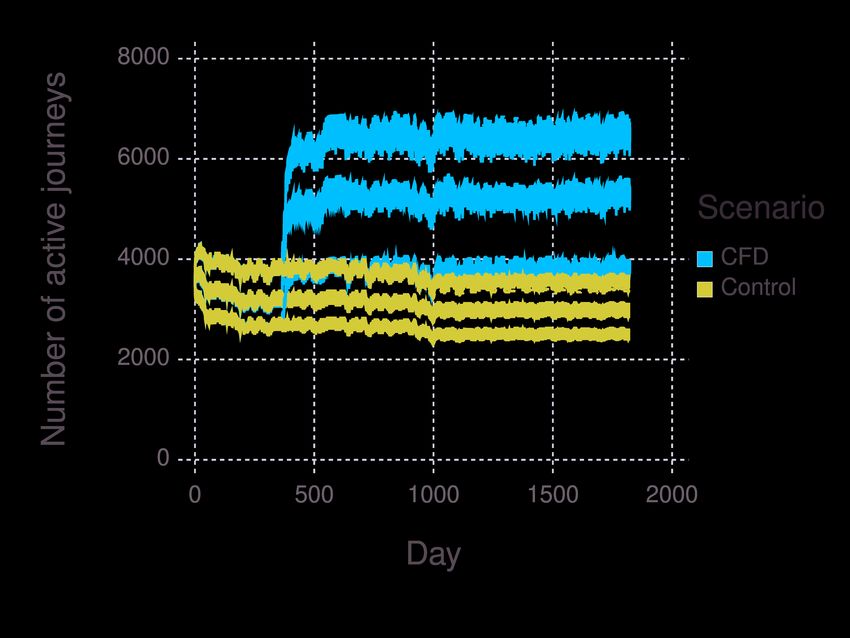
9tive commutes. Also, it appears to introduce more gests that targeted behaviour change programmes
instability, as shown in the figure. can change the behaviour of motivated subgroups,
Figure 2 shows the CFD scenario’s effect across resulting in shifts of around 5% of all trips at a
the 3 subcultures. In the control scenario, as ex- population level (Ogilvie et al., 2004). Interventions
pected, the pro-driving subculture (B) has the least that promote accessibility to active travel infras-
number of active journeys. This is followed by the tructure also appear to hold some promise (Panter
pro-cycling subculture (A) and then the pro-active- et al., 2019); if our model was to be calibrated with
travel subculture (C). The CFD intervention causes real-world environment data, it may be possible to
the pro-driving subculture (B) to perform more investigate the effect of changing the environmental
active journeys than the pro-active-travel subcul- supportiveness.
ture (C) in the control scenario. The others are Attempts to increase active commuting are not
greater in turn (C is greater than A which is greater always successful (Yang et al., 2010). Some interven-
than B). The gap between the subcultures is also tions, such as some built environment interventions
widened with the intervention having most effect in have worked well (Aldred et al., 2019). However,
the pro-active-travel group. other types of interventions have not (Martin et al.,
2012; Petrunoff et al., 2016; Sun et al., 2018). This
study has identified that a ‘nudge’ of car-free days,
4 Discussion in our model, causes a lasting change in behaviour.
As a result of people have fixed habits, unless they
This paper describes and presents MOTIVATE, an have a need to divert from their habit, they will
agent-based model which incorporates social norms not change from their preferred mode of transport.
related travel behaviour in simulations of the im- Car-free days are one kind of intervention which
pact of active commuting interventions. This model seeks to nudge people in to changing from habitual
serves as a tool, which could be populated with car use, our model shows it has the potential to have
real-world environment data, to investigate how so- a large relative effect. Car-free days are similar to
cial norms influence active travel interventions. We congestion charging in London, where areas of Cen-
demonstrated the utility of this model through the tral London (not including Waltham Forest) have
implementation of a scenario introducing car-free a £15 daily charge, with an additional £12.50 for
days against a control scenario. Overall, introduc- older vehicles (as of February 2022) in Inner London
ing car-free days on Wednesdays increased the odds (within the North and South Circular Roads). This
of active travel by 77.7% (OR 1.777; 89% HPDI: fiscal intervention attempts to push people in to not
[1.777, 1.777]) in the four years following interven- using their vehicle. This has been shown to cause
tion implementation. This is a large relative in- an increase in cycling, as people substitute vehicle
crease; however, absolute effects are modest, given use for bicycle use (Green et al., 2020).
that the odds of active commuting in the control Our model differs from existing models of trans-
scenario were 0.091 (89% HPDI: [0.091, 0.091]). We port systems (Axhausen and ETH Zürich, 2016;
simulated the impact of these interventions and Naiem et al., 2010; Hager et al., 2015; Bernhardt,
compared them to a control scenario. 2007), as it is not a traffic simulation – we do not
Car-free days force an individual to make a sig- aim to model traffic flow through a city. The in-
nificant change to commuting behaviour once per tended purpose of our model is not to make accurate
week. This constraint not only reduces the use of predictions of how people commute to work. Rather,
inactive commute modes on that specific day but the purpose is to explore how a range of diverse form
may also act as a ‘nudge’ to change overall commut- of inputs, including multiple social networks captur-
ing preferences by exposing individuals to active ing the effect of peers, as well as neighbours, habit,
commuting and shifting norms around active com- and variable environment parameters, such as the
muting on non-car-free days. This is shown in our weather, affect the decision to perform behaviour.
model, as on non-Wednesdays, in the car-free days For example, in 2 we show how the CFD intervention
intervention scenario, the odds of active travel were may affect members of different psychological sub-
70.3% (OR: 1.703; 89% HPDI: [1.703, 1.703]) greater cultures differently. We also see that habit causes
than the control scenario. Previous research sug- the CFD intervention to be sustained on non-car-
10Figure 1: 14 day moving average of active commutes separated by scenario and run. The scenarios
are CFD and Control. For 200 networks each with the same population, each scenario was run. The
weather pattern was kept constant across all runs. The dashed vertical line indicates the date at which
the intervention was introduced. n = 111 166 in all runs.
free days, where there were 70.3% (OR: 1.703; 89% that car-free days are effective. Such information,
HPDI: [1.703, 1.703]) move active journeys than the in the context of our model assumptions, may help
control scenario. This model can be used to ex- decision-makers better select and prioritise active
plore the effect of interventions on various aspects commuting interventions in the absence of a strong
of the decision-making process, such as habit, so- evidence base on intervention effectiveness. Such
cial networks, congestion, and the actions of peers models may also help research funders prioritise
and neighbours. This is a complement to models primary evaluations of potentially promising active
that more accurately model the spread of individ- commuting interventions identified by simulations
uals through urban environments. By combining (Ogilvie et al., 2020). This model may help to gen-
the evidence generated by real-world studies, traffic erate an understanding of currently radical policy
simulations, and simulations of the decision-making options – such as weekly car bans – and how the
process (such as ours), a greater understanding of underlying social structures impact the effectiveness
transport behaviour may be attained. of these interventions.
In common with all agent-based models, the re-
sults presented in this paper are not necessarily an 4.1 Strengths and limitations
accurate prediction of real-world intervention effects;
the only way to obtain this is to perform the inter- The strengths in this approach have been the use of
vention in the real-world. However, the utility of a microsimulation approach to generate a realistic
the presented model is in allowing the comparison of synthetic population for use in the model. This has
the relative effectiveness of a range of interventions been grounded in data from official statistics. The
under consistent model conditions in order to aid open-source nature of the model allows for refine-
public decision-making. In this study, we observe ment and adaptation of the MOTIVATE model and
11Figure 2: 14 day moving average of active commutes separated by scenario, run, and subculture (A / B /
C). The scenarios are CFD and Control. For 200 networks each with the same population, each scenario
was run. The weather pattern was kept constant across all runs. The dashed vertical line indicates the
date at which the intervention was introduced. n = 111 166 in all runs.
use of the model by other researchers or policymak- economic or social influences as part of the travel
ers for evaluation purposes. budget or travel cost as appropriate.
There are weaknesses in our approach which fur-
ther work could address. The environmental data
is not grounded in real data. Further work could
use geographic data to properly calibrate model The highest-posterior density intervals presented
inputs. It also only considers commuting behaviour; in the results cannot be interpreted as intervals of
personal journeys are excluded. Further work could what would happen in the real world. Normally,
be undertaken to extend the open-source model to statistical models directly model real-world data, as
allow for personal journeys to be modelled. Fur- such the statistical model is one of the real-world
thermore, it does not consider the processes which data-generating process, and assuming that the
may drive individuals to purchase cars or bicycles. model is not mis-specified intervals can be inter-
Encouraging people to purchase bicycles or give-up preted in the terms of the real world. This is not
cars may be a successful intervention, though our the case in this statistical model. Here, the statisti-
model cannot currently assess this. The fiscal cost cal model it is directly modelling results from the
of travel is also disregarded. Clearly, the financial agent-based model, and as such it can only be inter-
costs of travel is a major factor in deciding how to preted in terms of the simulated model ‘world’ – the
travel – if you cannot afford a car, you are unable agent-based model is the data-generating process.
to drive. Future work could consider how pricing In order to interpret it in terms of the real world,
affects commuting behaviour in the context of your we would need to strengthen the link between the
social environment as well as the built environment. simulated model world and the real-world through
There is room to include further environmental, further calibration and validation.
124.2 Conclusion Data accessibility
The MOTIVATE model and the findings presented The software and results are available to download
are an initial step in helping to improve under- under an open license (https://doi.org/10.5281/
standing in the design, prioritisation and impacts zenodo.5993329).
of active commuting interventions. The presented
agent-based model incorporates social norms related
to travel behaviour in order to provide a more realis- Competing interests
tic representation of the socio-ecological systems in
which active commuting interventions are deployed. We have no competing interests.
The utility of the model has been demonstrated
by simulating introducing car-free Wednesdays. In
silico studies are potentially a cost-effective way of References
aiding public health decision-making and setting
Rachel Aldred. ‘On the outside’: Constructing
research priorities. Utilising In silico studies, such
cycling citizenship. Soc Cult Geogr, 11(1):35–52,
as MOTIVATE and more traditional traffic sim-
2010. doi: 10.1080/14649360903414593.
ulations, could be a cost-effective way of aiding
public health decision-making and setting research Rachel Aldred and John Dales. Diversifying and nor-
priorities. It is also useful to see this ABM as a malising cycling in London, UK: An exploratory
representative of a new class of model that draws study on the influence of infrastructure. J Transp
on what we understand about both social and envi- Health, 4:348–362, 2017. doi: 10.1016/j.jth.2016.
ronmental effects in ways that point towards more 11.002.
actionable insights across a range of applications
not only in public health, but in any area where Rachel Aldred, James Woodcock, and Anna Good-
place-based and network-based effects overlap. man. Does More Cycling Mean More Diversity
in Cycling? Transp Rev, 34(1):28–44, 2016. doi:
10.1080/01441647.2015.1014451.
Authors’ contributions Rachel Aldred, Joseph Croft, and Anna Good-
man. Impacts of an active travel intervention
DL, JR, SM, and SC designed the study. DL per- with a cycling focus in a suburban context: One-
formed the synthetic population generation. All year findings from an evaluation of London’s in-
authors designed the agent-based model. RG im- progress mini-Hollands programme. Transp Res
plemented the agent-based model. RG conducted Part A Policy Pract, 123:147–169, 2019. doi:
the statistical analyses of the results. All authors 10.1016/j.tra.2018.05.018.
drafted and approved the manuscript.
Lars Bo Andersen. Active commuting is beneficial
for health. BMJ, 357:j1740, 2017. doi: 10.1136/
bmj.j1740.
Funding statement Kay W. Axhausen and ETH Zürich. The Multi-
Agent Transport Simulation MATSim. Ubiquity
This research was funded by KCL–LSHTM Press, August 2016. ISBN 978-1-909188-75-4. doi:
seed funding. RG is supported by a Medi- 10.5334/baw.
cal Research Council Studentship [grant number:
MR/N0136638/1]. SC is funded by Health Data Dag Balkmar. Towards an Intersectional Ap-
Research UK (HDR-UK). HDR-UK is an initiative proach to Men, Masculinities and (Un)sustainable
funded by the UK Research and Innovation, De- Mobility: The Case of Cycling and Modal
partment of Health and Social Care (England) and Conflicts. In Christina Lindkvist Scholten
the devolved administrations, and leading medical and Tanja Joelsson, editors, Integrating Gen-
research charities. der into Transport Planning : From One to
13Many Tracks. Palgrave Macmillan, 2019. doi: approach. Soc Sci Med, 65(9):1825–1838, 2007.
10.1007/978-3-030-05042-9_9. doi: 10.1016/j.socscimed.2007.05.036.
Albert-László Barabási and Réka Albert. Emer- Department for Transport. NTS0608: Bicycle own-
gence of Scaling in Random Networks. Science, ership by age: England, 2020.
286(5439):509–512, 1999. doi: 10.1126/science.
286.5439.509. Monica Dinu, Giuditta Pagliai, Claudio Macchi,
and Francesco Sofi. Active Commuting and Mul-
K Bernhardt. Agent-based modeling in transporta- tiple Health Outcomes: A Systematic Review and
tion. Artificial Intelligence in Transportation, 72, Meta-Analysis. Sports Med, 49:437–542, 2018. doi:
2007. 10.1007/s40279-018-1023-0.
Michael Betancourt. A Conceptual Introduction Mark Falcous. Why We Ride: Road Cyclists, Mean-
to Hamiltonian Monte Carlo. arXiv:1701.02434 ing, and Lifestyles. J Sport Soc Issues, 41(3):
[stat], July 2018. 239–255, 2017. doi: 10.1177/0193723517696968.
Jeff Bezanson, Alan Edelman, Stefan Karpinski, Tatiana Filatova, Peter H. Verburg, Dawn Cassan-
and Viral B. Shah. Julia: A Fresh Approach dra Parker, and Carol Ann Stannard. Spatial
to Numerical Computing. SIAM Review, 59(1): agent-based models for socio-ecological systems:
65–98, January 2017. ISSN 0036-1445, 1095-7200. Challenges and prospects. Environ Model Softw,
doi: 10.1137/141000671. 45:1–7, 2013. doi: 10.1016/j.envsoft.2013.03.017.
David J. Blok, Frank J. van Lenthe, and Sake J. de Ellen Flint and Steven Cummins. Active commut-
Vlas. The impact of individual and environmen- ing and obesity in mid-life: Cross-sectional, ob-
tal interventions on income inequalities in sports servational evidence from UK Biobank. Lancet
participation: Explorations with an agent-based Diabetes Endocrinol, 4(5):420–435, 2016. doi:
10.1016/S2213-8587(16)00053-X.
model. Int J Behav Nutr Phys Act, 15:107, 2018.
doi: 10.1186/s12966-018-0740-y. Ellen Flint, Steven Cummins, and Amanda Sacker.
Associations between active commuting, body fat,
Carlos A. Celis-Morales, Donald M. Lyall, Paul
and body mass index: Population based, cross
Welsh, Jana Anaderson, Lewis Steell, Yibing Guo,
sectional study in the United Kingdom. BMJ,
Reno Maldonado, Daniel F. Mackay, Jill P. Pell,
349:g4887, 2014. doi: 10.1136/bmj.g4887.
Naveed Sattar, and Jason M. R. Gill. Association
between active commuting and incident cardio- Ellen Flint, Elizabeth Webb, and Steven Cum-
vascular disease, cancer, and mortality: Prospec- mins. Change in commute mode and body-mass
tive cohort study. BMJ, 357:j1456, 2017. doi: index: Prospective, longitudinal evidence from
10.1136/bmj.j1456. UK Biobank. Lancet Public Health, 1(2):e46–e45,
2016. doi: 10.1016/S2468-2667(16)30006-8.
Christelle Clary, Daniel Lewis, Elizabeth Limb,
Claire M. Nightingale, Bina Ram, Angie S. Page, Hong Ge, Kai Xu, and Zoubin Ghahramani. Tur-
Ashley R. Cooper, Annew Ellaway, Billie Giles- ing: A Language for Flexible Probabilistic In-
Corti, Peter H. Whincup, Alicja R. Rudnicka, ference. In Amos Storkey and Fernando Perez-
Derek G. Cook, Christopher G. Owen, and Steven Cruz, editors, Proceedings of the Twenty-First
Cummins. Longitudinal impact of changes in the International Conference on Artificial Intelli-
residential built environment on physical activ- gence and Statistics, volume 84 of Proceedings
ity: Findings from the ENABLE London cohort of Machine Learning Research, pages 1682–1690.
study. Int J Behav Nutr Phys Act, 17:96, 2020. PMLR, April 2018.
doi: 10.1186/s12966-020-01003-9.
Andrew Gelman, John Carlin, Hal Stern, David
Steven Cummins, Sarah Curtis, Ana V. Diez-Roux, Dunson, Aki Vehtari, and Donald Rubin.
and Sally Macintyre. Understanding and repre- Bayesian Data Analysis. CRC Press, Boca Raton,
senting ‘place’ in health research: A relational FL, USA, third edition, 2014.
14Colin P. Green, John S. Heywood, and regional levels. J Transp Geogr, 34(C):282–296,
Maria Navarro Paniagua. Did the Lon- 2014. doi: 10.1016/j.jtrangeo.2013.07.008.
don congestion charge reduce pollution?
Reg Sci Urban Econ, 84:103573, 2020. doi: Glenn Lyons and Kiron Chatterjee. A human per-
10.1016/j.regsciurbeco.2020.103573. spective on the daily commute: Costs, benefits
and trade-offs. Transp Rev, 28(2):181–198, 2008.
Robert Greener, Daniel Lewis, Jon Reades, Simon doi: 10.1080/01441640701559484.
Miles, and Steven Cummins. Software and results
for: Incorporating social norms into a configurable Adam Martin, Marc Suhrcke, and David Ogilvie.
agent-based model of commuting behaviour, 2022. Financial Incentives to Promote Active Travel.
Am J Prev Med, 43(6):e45–e57, 2012. doi: 10.
Karsten Hager, Jürgen Rauh, and Wolfgang Rid. 1016/j.amepre.2012.09.001.
Agent-based modeling of traffic behavior in grow-
ing metropolitan areas. Transportation Research Nicholas D. Matsakis and Felix S. Klock. The
Procedia, 10:306–315, 2015. rust language. In HILT ’14: Proceedings of
the 2014 ACM SIGAda Annual Conference on
Jane Jacobs. The Death and Life of Great American High Integrity Language Technology, pages 103–
Cities. Jonathan Cape, London, 1962. 104, New York, NY, United States, November
James Jarrett, James Woodcock, Ulla K. Griffiths, 2014. Association for Computing Machinery. doi:
Zaid Chalabi, Phil Edwards, and Ian Roberts. 10.1145/2663171.2663188.
Effect of increasing active travel in urban England
Richard McElreath. Statistical Rethinking: A
and Wales on costs to the National Health Service.
Bayesian Course With Examples in R and Stan.
Lancet, 379(9832):2198–2205, 2012. doi: 10.1016/
Texts in Statistical Science. CRC Press, Boca
S0140-6736(12)60766-1.
Raton, FL, USA, second edition, 2020.
Matthew W. Knuiman, Hayley E. Christian, Mark L.
Met Office. Met Office Hadley Centre Observation
Divitini, Sarah A. Foster, Fiona C. Bull, Han-
Data, 2021.
nah M. Badland, and Billie Giles-Corti. A Longi-
tudinal Analysis of the Influence of the Neighbor- Graham F. Moore, Rhiannon E. Evans, Jemma
hood Built Environment on Walking for Trans- Hawkins, Hannah Littlecott, G. J. Melendez-
portation: The RESIDE Study. Am J Epidemiol, Torres, Chris Bonell, and Simon Murphy. From
180(5):453–461, 2014. doi: 10.1093/aje/kwu171. complex social interventions to interventions in
John Kruschke and an O’Reilly Media Company Sa- complex social systems: Future directions and un-
fari. Doing Bayesian Data Analysis, 2nd Edition. resolved questions for intervention development
2014. and evaluation. Evaluation, 25(1):23–45, 2019.
doi: 10.1177/1356389018803219.
Pietro Lanzini and Sana Akbar Khan. Shedding
light on the psychological and behavioral deter- Amgad Naiem, Mohammed Reda, Mohammed El-
minants of travel mode choice: A meta-analysis. Beltagy, and Ihab El-Khodary. An agent based
Transp Res Part F Traffic Psychol Behav, 48:13– approach for modeling traffic flow. In 2010 The
27, 2017. doi: 10.1016/j.trf.2017.04.020. 7th international conference on informatics and
systems (INFOS), pages 1–6. IEEE, 2010.
Robin Lovelace and Dimitris Ballas. ‘Truncate,
replicate, sample’: A method for creating integer Office for National Statistics. Location of usual
weights for spatial microsimulation. Comput En- residence and place of work by method of travel
viron Urban Syst, 41:1–11, 2013. ISSN 0198-9715. to work, 2014.
doi: 10.1016/j.compenvurbsys.2013.03.004.
Office for National Statistics, National Records of
Robin Lovelace, Dimitris Ballas, and Matt Watson. Scotland, and Northern Ireland Statistics and
A spatial microsimulation approach for the anal- Research Agency. 2011 Census aggregate data,
ysis of commuter patterns: From individual to 2017.
15David Ogilvie, Matt Egan, Val Hamilton, and Mark Felix Greaves, Laura Harper, Penelope Hawe,
Petticrew. Promoting walking and cycling as an Laurence Moore, Mark Petticrew, Eva Rehfuess,
alternative to using cars: Systematic review. BMJ, Alan Shiell, James Thomas, and Martin White.
329:763, 2004. doi: 10.1136/bmj.38216.714560.55. The need for a complex systems model of evidence
for public health. Lancet, 390(10112):2602–2604,
David Ogilvie, Adrian Bauman, Louise Foley, Cor- 2017. doi: 10.1016/S0140-6736(17)31267-9.
nelia Guell, David Humphreys, and Jenna Pan-
ter. Making sense of the evidence in population Harry Rutter, Nick Cavill, Adrian Bauman, and
health intervention research: Building a dry stone Fiona Bull. Systems approaches to global and na-
wall. BMJ Glob Health, 5:e004017, 2020. doi: tional physical activity plans. Bull World Health
10.1136/bmjgh-2020-004017. Organ, 97(2):162–165, 2019. doi: 10.2471/BLT.
18.220533.
Jenna Panter, Oliver Mytton, Stephen Sharp, Søren
Brage, Steven Cummins, Anthony A. Laverty, James F. Sallis, Ester Erin, Terry L. Conway,
Katrien Wijndaele, and David Ogilvie. Using Marc A. Adams, Lawrence D. Frank, and Michael
alternatives to the car and risk of all-cause, car- Pratt. Physical activity in relation to urban envi-
diovascular and cancer mortality. Heart, 104:1749– ronments in 14 cities worldwide: A cross-sectional
1755, 2018. doi: 10.1136/heartjnl-2017-312699. study. Lancet, 387(10034):2207–2217, 2016. doi:
10.1016/S0140-6736(15)01284-2.
Jenna Panter, Cornelia Guell, David Humphreys,
and David Ogilvie. Title: Can changing the Feiyang Sun, Peng Chen, and Junfeng Jiao. Pro-
physical environment promote walking and cy- moting Public Bike-Sharing: A Lesson from
cling? A systematic review of what works the Unsuccessful Pronto System. Transp Res
and how. Health Place, 58:102161, 2019. doi: Part D Transp Environ, 63:533–547, 2018. doi:
10.1016/j.healthplace.2019.102161. 10.1016/j.trd.2018.06.021.
Tamas K. Papp, Dilum Aluthge, JackRab, David University of Essex, Institute for Social and Eco-
Widmann, Julia TagBot, Morten Piibeleht, Pietro nomic Research, NatCen Social Research, and
Monticone, and St–. Tpapp/DynamicHMC.jl: Kantar Public. Understanding Society: Waves
V3.1.1. Zenodo, October 2021. 1–10, 2009–2019 and Harmonised BHPS: Waves
1–18, 1991–2009, 2020.
Richard Patterson, Jenna Panter, Eszter P. Vamos,
Steven Cummins, Christopher Millett, and An- Duncan J. Watts and Steven H. Strogatz. Collective
thony A. Laverty. Associations between commute dynamics of ‘small-world’ networks. Nature, 393:
mode and cardiovascular disease, cancer, and 440–442, 1998. doi: 10.1038/30918.
all-cause mortality, and cancer incidence, using
linked Census data over 25 years in England and World Health Organization. Physical
Wales: A cohort study. Lancet Planet Health, 4 Activity. https://www.who.int/news-
(5):e186–e194, 2020. doi: 10.1016/S2542-5196(20) room/fact-sheets/detail/physical-activity,
30079-6. 2020. Archived at https://web.archive.
org/web/20220215115309/https://www.
Nick Petrunoff, Chris Rissel, and Li Ming Wen. The who.int/news-room/fact-sheets/detail/
Effect of Active Travel Interventions Conducted in physical-activity.
Work Settings on Driving to Work: A Systematic
Review. J Transp Health, 3(1):61–76, 2016. doi: Lin Yang, Shannon Sahlqvist, Alison McMinn, Si-
10.1016/j.jth.2015.12.001. mon J. Griffin, and David Ogilvie. Interventions
to Promote Cycling: Systematic Review. BMJ,
Roads Task Force. Who travels by car in London and 341:c5293, 2010. doi: 10.1136/bmj.c5293.
for what purpose? Technical Note 14, Transport
for London, 2013. Yong Yang and Ana V. Diez-Roux. Using an agent-
based model to simulate children’s active travel
Harry Rutter, Natalie Savona, Ketevan Glonti, to school. Int J Behav Nutr Phys Act, 10:67, 2013.
Jo Bibby, Steven Cummins, Diane T. Finegood, doi: 10.1186/1479-5868-10-67.
16You can also read