Journal of the Mechanics and Physics of Solids - Sites at USC
←
→
Page content transcription
If your browser does not render page correctly, please read the page content below
J. Mech. Phys. Solids 151 (2021) 104382
Contents lists available at ScienceDirect
Journal of the Mechanics and Physics of Solids
journal homepage: www.elsevier.com/locate/jmps
Mechanics of photosynthesis assisted polymer strengthening
Kunhao Yu, Zhangzhengrong Feng, Haixu Du, Qiming Wang *
Sonny Astani Department of Civil and Environmental Engineering, University of Southern California, Los Angeles, CA 90089, United States
A R T I C L E I N F O A B S T R A C T
Keywords: Plant cells utilize photosynthesis to produce glucose that is delivered to selected locations to form
Self-strengthening stiff polysaccharides (e.g., chitin, chitosan, and cellulose), which strengthen the plant structures.
Photosynthesis Such a photosynthesis-assisted strengthening behavior in plants has rarely been imitated in
Glucose
synthetic material systems. We here propose a synthetic polymer system embedded with
Polymer network model
Engineered living materials
extracted plant chloroplasts, which allow for the photosynthesis-assisted mechanical strength
ening of the polymer matrix. The strengthening mechanism relies on an additional crosslinking
reaction between the photosynthesis-produced glucose and side groups within the polymer ma
trix. We develop a theoretical framework to model the photosynthesis-assisted strengthening
behaviors of polymers. The glucose production of the embedded chloroplasts will be first modeled
with a general photosynthesis theory, and the exportation of glucose to the polymer matrix is
modeled with an enzyme-assisted mass transport theory. Next, a polymer strengthening network
model with glucose molecules as additional crosslinkers is presented. Effects of the illumination
period, the concentration of embedded chloroplasts, and the light intensity on the stiffness
strengthening are studied. The theoretical results consistently agree with the experimental results
of the photosynthesis-assisted polymer strengthening.
1. Introduction
Plants offer continuous sources of inspiration for the engineering endeavor. Engineering materials inspired by plants provide great
promise for designing and optimizing material properties and functionalities, such as hydrophobicity (Barthlott et al., 2010; Tricinci
et al., 2015; Zeiger et al., 2016), mechanical properties (Gan et al., 2019; Li and Wang, 2015b; Sehaqui et al., 2010), remodeling (Del
Dottore et al., 2018), self-healing (Yu et al., 2020a,2019b), and shape-changing (Armon et al., 2011; Correa et al., 2015; Li and Wang,
2015a, b). Of particular interest is plants’ strengthening behavior: Plant cells utilize photosynthesis to produce glucose that is delivered
to selected locations to form stiff polysaccharides (e.g., chitin, chitosan, and cellulose), which strengthen the plant structures (Fig. 1a)
(Barthelemy and Caraglio, 2007; Popper et al., 2011). For example, the stiffness of a young stem is typically in the order of kilopascal,
while the stiffness of a mature trunk can reach as high as several gigapascals (Shah et al., 2017). Although such a
photosynthesis-assisted strengthening behavior is the basis of plants’ growth and remodeling, how to imitate such strengthening
behavior in a synthetic material system remains largely elusive.
Here, we propose a synthetic polymer system embedded with extracted plant chloroplasts, which allow for the photosynthesis-
assisted mechanical strengthening of the polymer matrix (Fig. 1b)(Yu et al., 2021). The strengthening mechanism relies on an
additional crosslinking reaction between the photosynthesis-produced glucose and side groups within the polymer matrix, thus
* Corresponding author.
E-mail address: qimingw@usc.edu (Q. Wang).
https://doi.org/10.1016/j.jmps.2021.104382
Received 1 December 2020; Received in revised form 12 February 2021; Accepted 25 February 2021
Available online 27 February 2021
0022-5096/© 2021 Elsevier Ltd. All rights reserved.
K. Yu et al. Journal of the Mechanics and Physics of Solids 151 (2021) 104382
forming a stiff region with additional crosslinks (Fig. 1b). This material system provides a unique platform for strengthening and
remodeling engineering materials via the communication between synthetic polymers and natural photosynthesis processes, thus
opening the door for the design of hybrid synthetic-living materials, for applications such as smart composites and soft robotics.
Moreover, the photosynthesis-assisted strengthening can usually be delivered locally to achieve on-demand strengthening perfor
mance, or to impart graded stiffness with graded light intensity, which has been a longstanding challenge in traditional fabrication
processes that require continuously switching materials during fabrication (Bartlett et al., 2015). Despite the great potential, the
fundamental understanding of this class of hybrid synthetic-living materials with living chloroplasts has been left behind due to two
key reasons. First, the underlying mechanism between the living chloroplasts and the synthetic polymer system hasn’t been well
understood. Although several biochemical models have been proposed to capture the photosynthesis behavior of plants (Farquhar
et al., 1980; Zhu et al., 2013), there is no theoretical model to quantitatively understand the photosynthesis process of extracted
chloroplasts within a polymer matrix. It remains elusive how photosynthesis-produced glucose molecules interact with the polymer
network. It is also unclear how to mechanistically understand the effects of the concentration and photosynthesis conditions of
embedded chloroplasts on the material strengthening behavior. Second, the understanding of strengthening networks based on
additional crosslinking remains elusive. How the additional crosslinks affect the existing polymer networks remains unknown. How
Fig. 1. (a) Schematics to illustrate photosynthesis-assisted remodeling of plants. The photosynthesis-produced glucose undergoes a condensation
reaction to form stiff polysaccharides (e.g., cellulose). (b) Schematics to illustrate photosynthesis-assisted remodeling of a synthetic polymer. The
photosynthesis-produced glucose undergoes a reaction with isocyanate (NCO) side groups to form additional crosslinks. (c) Schematic and sample
with free NCO groups and embedded chloroplasts before and after undergoing 4-h light illumination and 4-h darkness. (d) Uniaxial tensile stress-
strain curves of one experimental group and two control groups. The experimental group includes samples with free NCO groups and embedded
chloroplasts undergoing 4-h light illumination and 4-h darkness. The control 1 group includes samples with free NCO groups and embedded
chloroplasts undergoing 8-h darkness. The control 2 group includes samples with free NCO groups but without chloroplasts undergoing 4-h light
illumination and 4-h darkness. (e) Young’s moduli of three groups of samples.
2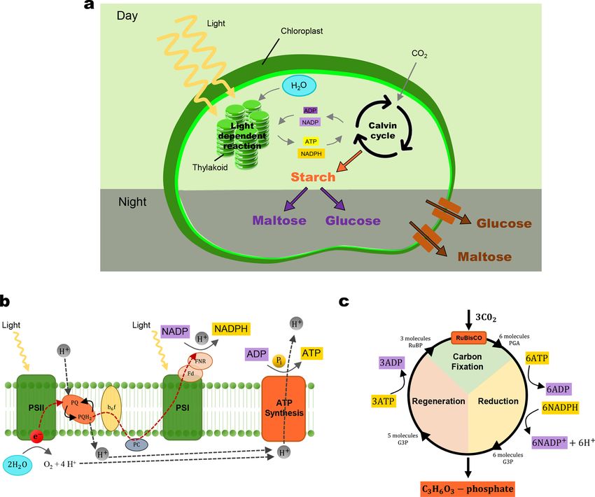
K. Yu et al. Journal of the Mechanics and Physics of Solids 151 (2021) 104382
the additional crosslinks affect the polymer chain evolution is also ambiguous. The missing of these aspects of theoretical under
standing would significantly drag down the innovation of photosynthesis-assisted hybrid synthetic-living materials.
In this paper, we present a theoretical framework to model the self-strengthening behaviors of polymers assisted by the photo
synthesis process. The strengthening mechanism of the synthetic polymer is shown in Fig. 1b. The photosynthesis-produced glucose
can facilitate additional crosslinking reactions in the polymer matrix upon exposure to white light. The photosynthesis-assisted
crosslinking is forming due to the reaction of open free isocyanate (NCO) groups in the material matrix and hydroxyl (OH) groups
on the glucose, which enables the enhancement of mechanical properties of materials including Young’s modulus and tensile strength
(Figs. 1c-e). The photosynthesis-assisted glucose production of the embedded chloroplasts will be first modeled with a general
photosynthesis theory. Then, the exportation of glucose from the chloroplasts to the polymer matrix is modeled with an enzyme-
assisted mass transport theory. Next, the original polymer matrix is modeled with a network model with homogeneous chain
length distribution. When the photosynthesis-produced glucose is introduced in the polymer matrix and form the additional crosslinks,
inhomogeneous chain lengths are considered following two different algorithms. The formation of additional crosslinks will be
examined by the comparison between experimental and theoretical results. Effects of the illumination period, the concentration of
embedded chloroplasts, and the light intensity on the stiffness strengthening will be studied. The theoretical model can consistently
explain experimentally observed photosynthesis-assisted strengthening.
The plan of the paper is as follows. Section 2 introduces the experiments about the photosynthesis-assisted strengthening of a
chloroplast-embedded polymer system. In Section 3, we present the theoretical model system by first considering the general theory
for the photosynthesis process in the material matrix, then the model for polymer strengthening by additional crosslinking. In Section
4, we present the theoretical results from the photosynthesis model and then from the polymer strengthening model. With respective
experiments and theories, the effects of the illumination period, the concentration of embedded chloroplasts, and the light intensity
will be studied. The concluding remarks will be presented in Section 5.
2. Experimental
The polymer was prepared by embedding the extracted chloroplasts in a synthetic polymer matrix. The polymer with free NCO
groups was prepared by preheating 0.01 mole of Poly(tetrahydrofuran) (PolyTHF, average molar mass 650 g/mol) at 100 ◦ C, and
exposed to the nitrogen environment for 1 h to remove moisture and oxygen. 0.02 mole of isophorone diisocyanate (IPDI), 10 wt% of
dimethylacetamide (DMAc), and 1 wt% of dibutyltin dilaurate (DBTDL) were mixed with the preheated PolyTHF at 70 ◦ C, and stirred
with a magnetic stir bar for 1 h. After reducing the temperature to 40 ◦ C, 0.01 mole of 2-Hydroxyethyl methacrylate (HEMA) was
added and mixed for 1 h to complete the synthesis (0.02 mole of HEMA was added for the polymer without free NCO groups). Then, we
extracted living chloroplasts from spinach leaves (Joly and Carpentier, 2011). The HEPES buffer solution was prepared by mixing
HEPES buffer (30 × 10− 3 M, pH 5.0–6.0), poly(ethylene glycol) (Mw. 8000, 10% (w /v)), MgCl2 (2.5 × 10− 3 M), K3 PO4 (0.5 ×
10− 3 M), and DI Water. The HEPES buffer solution was then magnetically stirred for 3 h. NaOH solution was added to adjust the pH
value to be around 7.6. The HEPES buffer solution was then stored in the fridge at 4 ◦ C for 3 h before use. Then, the fresh baby spinach
leaves (Spinacia oleracea L.) were washed with DI water and then dried to remove the surface water. Next, the middle veins of the
leaves were removed to obtain 65 g leaf meat from about 100 g of fresh leaves. Then, the leaf meat was ground with 100 ml HEPES
buffer solution in the pre-chilled kitchen blender for about 2 min until the mixture became homogeneous. The mixture was centrifuged
with 4000 RPM for 15 min at 4 ◦ C (Eppendorf 5804R). Then, the supernatant was removed, and the chloroplast pellet was
re-suspended in the HEPES buffer solution. After adding the suspended mixture on the top of 5 mL of 40% Percoll in two pre-chilled
tubes, we centrifuged the mixture at 3636 RPM for 8 min at 4 ◦ C. Later, we removed the supernatant and kept the pellet. Next, we
washed the pellet by adding 10 mL HEPES buffer solution and piped it out twice to remove Percoll. Before using the extracted
chloroplast, we put the tubes upside down in the fridge for 1 h to get rid of the remained water or buffer solution from the chloroplast
pellet. Extracted chloroplasts of various weight percent from 0 wt% to 5 wt% were gently mixed with the prepared polymer inks (with
or without free NCO groups) using a magnetic stir bar for 30 min at 4∘ C in a dark environment to prevent the degradation of chlo
roplasts. Then, 2 wt% of photoinitiator (phenylbis(2,4,6-trimethylbenzoyl) phosphine oxide) was mixed with the polymer inks. The
polymer was fully cured under white light from a white-light projector for 60 s.
To allow for the photosynthesis process, we placed the prepared chloroplast-embedded polymer samples in a white-light chamber
(CL-1000 Ultraviolet Crosslinker with five UVP 34–0056–01 bulbs, light intensity 69.3W/m2 ) and undergone various light illumi
nation periods (0–4 h) and the respective darkness periods (same length of the illumination period). For example, the 15-min group
went through 15-min light illumination and 15-min darkness. For the samples with various weight concentrations (0–5 wt%) of
chloroplasts, they went through 4-h light illumination and 4-h darkness. After the illumination and darkness process, the samples were
then uniaxially stretched until rupture with a strain rate of 0.05 s− 1 with a mechanical tester (Instron, model 5942). The Young’s
modulus of each sample was calculated from the obtained tensile stress-strain curves (Figs. 1de).
To verify that photosynthesis can indeed assist the polymer strengthening, we study three sample groups for comparison: The
experimental group includes polymer samples with free NCO groups and embedded chloroplasts, going through 4-h illumination and
4-h darkness, control 1 group that includes polymer samples with free NCO groups and embedded chloroplasts, going through 8-h
darkness, and control 2 group that includes polymer samples with free NCO groups but without chloroplasts, going through 4-h
light illumination and 4-h darkness. We compare the mechanical properties of three sample groups via uniaxial tensile tests
(Fig. 1d). Compared to controls 1 and 2, the experimental group exhibits higher Young’s modulus by a factor of 620% (Fig. 1e) and
higher tensile strength by a factor of 350%.
3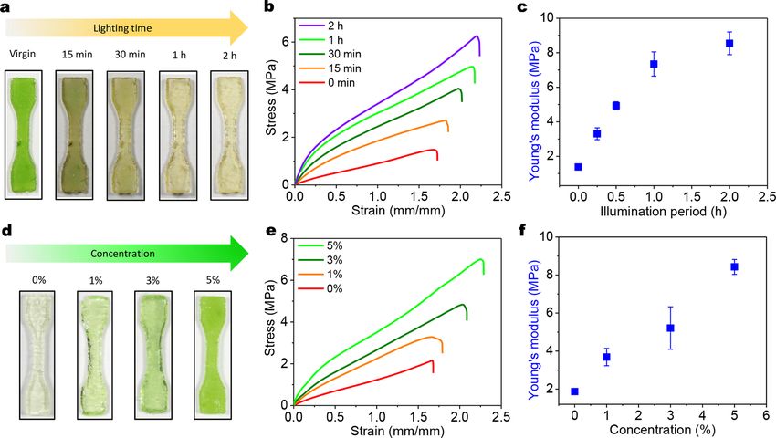
K. Yu et al.                                                                               Journal of the Mechanics and Physics of Solids 151 (2021) 104382

    In addition, we study the effects of two vital factors on the strengthening performance: concentration of embedded chloroplasts and
light illumination period (Fig. 2). First, we employ various light illumination periods (white light intensity 0–69.3 W /m2 ) to process
the polymer samples with 5 wt% chloroplasts and free NCO groups. Tensile stress-strain curves show that Young’s moduli increase
with increasing illumination time within 0–2 h (Fig. 2a-c). Then, we investigate polymer samples with chloroplasts of various weight
concentrations (0–5 wt%) and free NCO groups (processed with 4-h illumination and 4-h darkness). Tensile stress-strain curves show
that Young’s moduli increase with increasing chloroplast concentrations over 0–5 wt%, (Figs. 2d-f).

3. Theoretical model

   In this section, we will establish a theoretical framework to understand the fundamental mechanics of photosynthesis-assisted
polymer strengthening. The theory will explain the mechanisms of two processes: (1) Glucose is produced by the photosynthesis
process within chloroplasts and then exported from the chloroplasts to the polymer matrix (Section 3.1), and (2) additional crosslinks
are formed within the polymer network through the reaction between glucose and the NCO side groups (Section 3.2).

3.1. Part 1: glucose production and exportation

   With the extracted chloroplasts embedded in the polymer matrix, the energy from light can trigger the photosynthesis process to
produce glucose. The overall process of photosynthesis is shown in Fig. 3a (Gregory, 1977; Lawlor, 1993). During the daytime,
chloroplasts first convert light energy to the energy-carrier molecules, and these molecules are simultaneously used to produce starch
that is stored in the chloroplast. During the night, the accumulated starch is broken down as glucose and exported out of the chloroplast
(Fig. 3a). In Section 3.1.1, we will model the conversion of light energy to chemical energy by considering a light-dependent reaction
(Fig. 3b). In Section 3.1.2, we will model the production of starch by considering a photosynthetic carbon reduction (PCR) cycle or
usually called the Calvin cycle (Fig. 3c). In Section 3.1.3, we will model the starch degradation and glucose export by using the
Michaelis-Menten kinetic.

3.1.1. Kinetics of the light-dependent reaction
    In the light-dependent reaction, the pigment chlorophyll can convert light energy to chemical energy in the form of adenosine
triphosphate (ATP) and nicotinamide adenine dinucleotide phosphate (NADPH) (Fig. 3b), which are later used to produce glucose in
the next stage of photosynthesis (Gregory, 1977; Lawlor, 1993). Photochemically, one molecule of the pigment chlorophyll absorbs

Fig. 2. (a) Samples with 5 wt% chloroplasts after the photosynthesis processes with various light illumination periods. (b) Uniaxial tensile stress-
strain curves, (c) Young’s moduli of samples with 5 wt% chloroplasts after the photosynthesis processes with various light illumination periods. Note
that each light illumination period follows up with the same period of darkness period. (d) Samples with embedded chloroplasts of various weight
concentrations. (e) Uniaxial tensile stress-strain curves, (f) Young’s moduli of various weight concentrations samples undergo 4-h light illumination
and 4-h darkness.

                                                                         4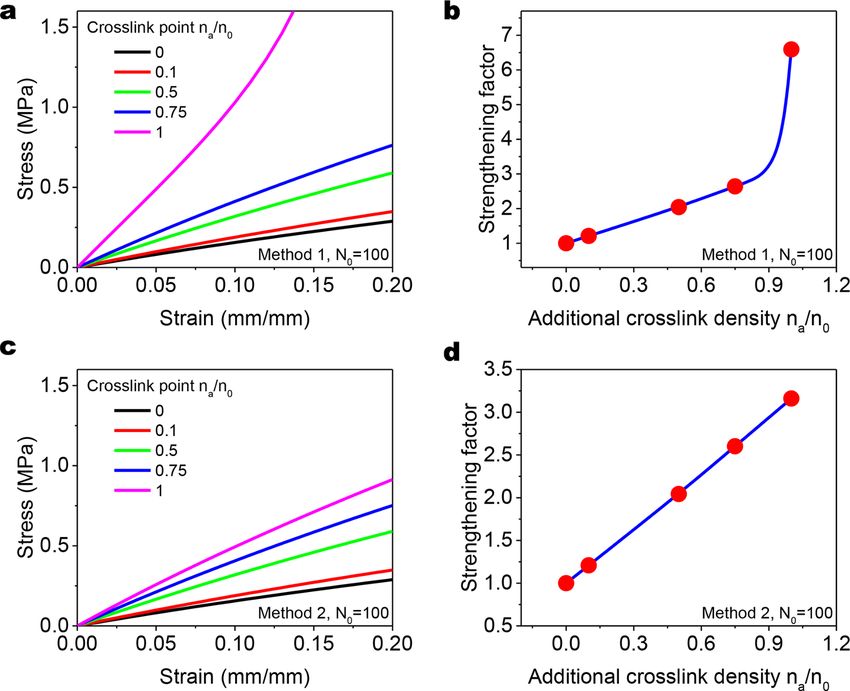
K. Yu et al. Journal of the Mechanics and Physics of Solids 151 (2021) 104382
Fig. 3. Schematics of chloroplast to illustrate (a) overall photosynthesis process during day and night (b) light-dependent reaction (c) photosyn
thetic carbon reduction (PCR) cycle.
one photon and loses one electron (Von Caemmerer, 2000). This electron transfers to a modified form of chlorophyll called pheo
phytin, which passes the electron to a quinone molecule, starting the flow of electrons down to an electron transport chain that leads to
the ultimate reduction of NADP to NADPH (Fig. 3b). In addition, this process creates a proton gradient (energy gradient) across the
chloroplast membrane, which is used by photophosphorylation in the synthesis of ATP (Fig. 3b). The chlorophyll molecule ultimately
regains the electron when a water molecule is split in a process called photolysis (or water splitting), which releases a dioxygen (O2 )
molecule. The overall equation of the light-dependent reaction is written as
2 H2 O + 2 NADP+ + 3 ADP + 3 Pi + 4 hν → 2 NADPH + 2 H+ + 3 ATP + O2 (1)
The net-reaction can be reduced as (Barber, 2017; Kok et al., 1970; Von Caemmerer, 2000; Yeung et al., 2015)
2 H2 O + 4 hν → 4 H+ + O2 (2)
We consider a light source with an initial light intensity I0 is illuminated on a polymer matrix with embedded chloroplasts. Due to
the semitransparent color of the chloroplast-embedded sample, the light propagation will be attenuated through the polymer matrix,
which can be described with the Beer-Lambert law (Long et al., 2011, 2009, 2013; Yu et al., 2019a),
∂I(z)
= − AI(z) (3)
∂z
where the light illumination is along the z-axis, I(z, t) is the light intensity at position z along the z-axis at time t, A is the absorption
coefficient of the material. The light propagation direction is along a single axis (the z-axis); thus, we consider the light attenuation as a
5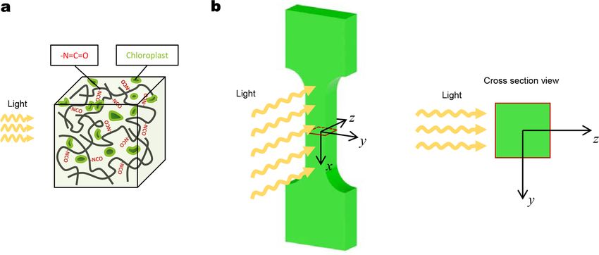
K. Yu et al. Journal of the Mechanics and Physics of Solids 151 (2021) 104382
1D problem (Fig. 4). The absorption coefficient can be estimated as (Vogelmann and Evans, 2002)
A = α1 η (4)
where α1 is the light absorption coefficient, and η is the mass concentration of the chloroplast within a unit volume of material (e.g.,
0–5%, dimensionless). Here, we assume the polymer is incompressible, and thus the amount of chloroplast per unit volume will remain
constant throughout the deformation.
With a constant initial light intensity I0 , the light intensity along the sample thickness direction (z-axis) can be written as (Eq. (3)
and Fig. 4b),
I(z) = I0 exp(− Az) (5)
The chloroplasts embedded in the matrix absorb the photons via pigment chlorophyll and release electrons in the chloroplast. The
governing equation of the absorbed photon concentration by the chlorophyll Cp (z, t) can be written as (Long et al., 2011, 2009, 2013;
Yu et al., 2019a; Zhao et al., 2015),
∂Cp (z, t) 1 I(z)
= εc ηM α2 (6)
∂t NA hc/λ
where εc is the photosynthetic energy conversion efficiency of photon energy, ηM (mol/m3) is the molar concentration of the chlo
rophyll, α2 is the molar absorptivity of chlorophyll, NA = 6.02 × 10²³ mol− 1 is the Avogadro number, h = 6.63 × 10− 34 Js is the
Plank constant, c = 3 × 10⁸ ms− 1 is the speed of light, and λ = 550 nm is the mean wavelength of white light. Note that, ηM should be
in a linear relationship with η, i.e., ηM = φη, where φ ≈ 2.2 × 10− 3 mol/m3 (Von Caemmerer, 2000). In practice, chloroplasts do not
convert all radiation energy into biomass energy, mainly due to the respiration requirements, reflection, and the need for optimal solar
radiation levels. The overall photosynthetic efficiency is estimated between 3 and 6% of total photon energy (Bugbee and Salisbury,
1988; Zhu et al., 2010).
From Eqs. (1) and (2), the absorbed photon by the chlorophyll is used to create a proton gradient and then store the biomass energy
in the chemical forms of ATP and NADPH. Since the formation of ATP and NADPH both require protons, to simplify the problem, we
here consider the production of protons CH+ as an irreversible chemical kinetic with photon energy to represent the formation of ATP
and NADPH written as (Lei et al., 2007)
∂CH+
= k1 Cp (z, t) (7)
∂t
where k1 (s− 1 ) is the reaction rate to produce protons.
3.1.2. Photosynthetic carbon reduction (PCR) cycle
After the NADPH and ATP are generated from the light-dependent reaction, these energy-carrier molecules are simultaneously used
to produce the glucose through the photosynthetic carbon reduction cycle (PCR cycle). In the PCR cycle, an enzyme called RuBisCO
captures carbon dioxide from the atmosphere and uses the energies from NADPH and ATP to release hydrocarbon sugar (Fig. 3c).
Fig. 4. (a) Schematics to illustrate the experiment procedure of light illuminate on the sample. (b) The global Cartesian coordinate system is
constructed on the testing area. The light illumination direction is along the z-axis.
6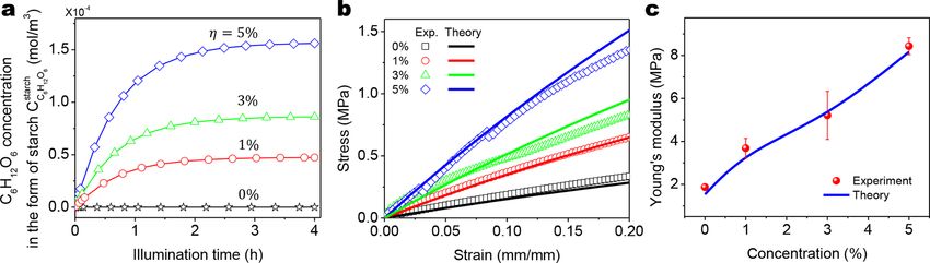
K. Yu et al. Journal of the Mechanics and Physics of Solids 151 (2021) 104382
During the daytime, the released hydrocarbon sugar is temporarily stored in the chloroplast in the form of starch (Graf et al., 2010;
Smith et al., 2005). The overall equation for PCR cycle is written as (Gregory, 1977; Lawlor, 1993; Von Caemmerer, 2000)
(8)
RuBisCO
3 CO2 + 2 ATP + 6 NADPH + 6 H+ ̅̅̅→ C3 H6 O3 − phosphate + 2 ADP + 8 Pi + 3 H2 O + 6 NADP+
Eq. (8) can be reduced by normalizing the coefficients as
1 RuBisCO 1 1
CO2 + H+ ̅̅̅→ C6 H12 O6 + H2 O (9)
4 24 4
The chemical kinetics between proton (H+ ) and the produced C6 H12 O6 in the form of starch during PCR cycle can be explained by
the enzyme activity of RuBisCO following the Michaelis-Menten kinetics (Flamholz et al., 2019; Kubien et al., 2008; Zhu et al., 1998),
written as,
( / ) ( )
∂ CCstarch
6 H12 O6
24 kcat1 CRubisco CH+ CCstarch
= − kt 6 H12 O6
(10)
∂t CH+ + kM1 24
where Cstarch − 1
C6 H12 O6 is the concentration of the produced C6 H12 O6 in the form of starch, kcat1 (s ) is the catalytic rate of RuBisCO, CRubisco is
the concentration of the enzyme RuBisCO, kM1 is the Michaelis constant of RuBisCO, and kt is the termination rate of starch synthesis.
We assume the gradually increased accumulation of starch in the chloroplast will result in termination of starch production, which has
been found as a self-limiting process once the chloroplasts become saturated with transitory starch (Longland and Byrd, 2006). Note
that the formation of starch typically requires a condensation reaction between a number of C6 H12 O6 molecules, which kick out water
molecules (Gregory, 1977; Lawlor, 1993; Von Caemmerer, 2000). However, the molar mass of starch is typically unknown; therefore,
we only consider the amount of the smallest unit C6 H12 O6 within the starch, but not directly consider the amount of the large starch
molecule.
The production of starch during the photosynthesis process involves both the light-dependent reaction and the PCR cycle. The
photon energy will first facilitate the production of biomass energies in the light-dependent reaction, and the enzyme will then
facilitate the biomass energies to produce starch stored in the chloroplast (Smith et al., 2005). Therefore, these two processes are
strongly coupled. Light can facilitate the production of biomass energy, and at the same time, the biomass energies are utilized by the
enzyme to produce starch. This kinetic equation can effectively represent the overall photosynthesis chemical reaction, which is
summarized as (Gregory, 1977; Lawlor, 1993; Von Caemmerer, 2000)
(11)
12hν
6 H2 O + 6 CO2 ̅→ C6 H12 O6 + 6 O2
3.1.3. Glucose exportation to matrix
During the night (darkness period), the accumulated starch in the chloroplast is first broken down into simple sugar such as maltose
and glucose, which are then exported through the chloroplast membrane to the polymer matrix by glucose transporter (Fig. 3a)
(Schafer et al., 1977; Servaites and Geiger, 2002). It is noteworthy that both maltose and glucose molecules have hydroxyl groups
(OH), which can have a strong reaction with NCO groups within the initial polymer network. Since glucose is the simplest form of sugar
and maltose is merely a form of multiple condensed glucose molecules, for simplicity, we here consider the product exported from the
chloroplasts is glucose.
The breaking-down process of starch to form glucose molecules can be considered as a simple relationship with the darkness time
(Chew et al., 2014; Graf et al., 2010; Lu et al., 2005), written as
dCgin dCCstarch
=− 6 H12 O6
= kd CCstarch
6 H12 O6
(12)
dt dt
where Cgin is the concentration of glucose in the chloroplasts, kd is the degradation rate of starch and Cstarch
C6 H12 O6 is the C6 H12 O6 con
centration in the form of starch.
The glucose molecules can be transported across the membrane of the chloroplast, assisted by the transportation enzyme (Nag
et al., 2011). The enzyme-catalyzed transportation of glucose from chloroplast to material matrix can be explained with the
Michaelis-Menten kinetics (Nag et al., 2011), written as
dN kcat2 Ctrans Cgin
= (13)
dt Cgin + kM2
where dN/dt is the export rate of the glucose through the membrane transporter, kcat2 is the catalytic rate of glucose transport, Ctrans is
the concentration of transportation enzyme, and kM2 is the Michaelis constant of the enzyme. The incremental concentration of glucose
per unit volume in the material matrix can thus be calculated as
dN 1 kcat2 Ctrans Cgin
= dt (14)
Vout Vout Cgin + kM2
where Vout is a unit volume of the material matrix. Therefore, the total concentration of glucose in a unit volume of the material matrix
7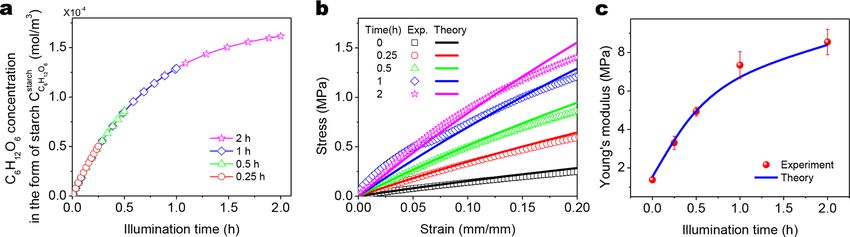
K. Yu et al. Journal of the Mechanics and Physics of Solids 151 (2021) 104382
at darkness time tdark can be calculated as
∫tdark ∫tdark
1 1 kcat2 Ctrans Cgin
Cgout = dN = dt (15)
Vout Vout Cgin + kM2
0 0
Note that the chloroplast-produced glucose in the material matrix is a function of light intensity, light illuminating time, darkness
time, and concentration of the embedded chloroplasts. We will further discuss the effects of these factors on the strengthening be
haviors in Section 4.
3.2. Part 2: polymer strengthening by additional crosslinking
The initial polymer matrix is first crosslinked by the photoradical initiated addition reaction of the acrylate groups (Fig. 5a). Within
this initial polymer network, NCO groups are active sites that can have a strong reaction with hydroxyl groups (OH) on the chloroplast-
produced glucose to form urethane linkages (-NH–CO–O-). We here consider these newly formed urethane linkages as the new
crosslinks additional to the acrylate-enabled crosslinks within the designed polymer matrix. In Section 3.2.1, we will first model the
initial polymer network by considering a homogeneous chain length distribution network model; and in Section 3.2.2, we will model
the strengthening of material by considering the formation of inhomogeneous chain lengths due to the additional crosslinks.
3.2.1. Initial polymer network
Before strengthening, the polymer network is assumed to feature a homogenous chain length. The chain length is described by the
Kuhn length, denoted as N0 and chain number per unit volume as n0 . The strain energy density of the polymer network can be written
Fig. 5. (a) Schematics to show the formation of additional crosslinks through the reaction between the free NCO groups and the glucose. (b)
Schematics to show the formation of one crosslink between two chains with the length of N0 . We assume each chain with the initial length of N0
becomes two chains with the length of N0 /2. (c) Schematics to show the formation of one crosslink between a chain with the length of N0 /2i and a
chain with the length of N0 /2j . We assume the crosslink formed between a chain with the length of N0 /2i and a chain with the length of N0 /2j
induces four chains with respective half lengths, where i = 0, 1, 2⋯ and j = 0, 1, 2⋯.
8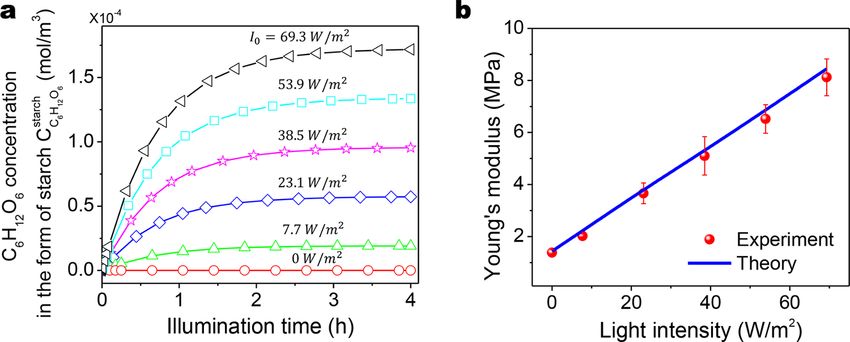
K. Yu et al. Journal of the Mechanics and Physics of Solids 151 (2021) 104382
as (Arruda and Boyce, 1993; Treloar, 1975)
( )
β0 β0
W0 = n0 kB TN0 + ln (16)
tanhβ0 sinhβ0
where kB is the Boltzmann constant, T is the temperature in Kelvin, and
( )
Λ
β0 = L− 1 √̅̅̅̅̅̅ (17)
N0
where L− 1 () is the inverse Lagrange function and Λ is the chain stretch. Here, we follow an affine deformation assumption that the
microscopic deformation at the polymer chain level affinely follows the macroscopic deformation at the material level in three
principal directions; therefore, the chain stretch can be expressed as
√̅̅̅̅̅̅̅̅̅̅̅̅̅̅̅̅̅̅̅̅̅̅̅̅
Λ = λ21 + λ22 + λ23 (18)
This affine deformation assumption has been widely adopted for deriving the constitutive models for rubber-like materials, such as
neoHookean model (Treloar, 1975) and Arruda-Boyce model (Arruda and Boyce, 1993). Note that Eq. (18) is slightly different from
√̅̅̅̅̅̅̅̅̅̅̅̅̅̅̅̅̅̅̅̅̅̅̅̅̅̅̅̅̅̅̅̅̅̅
the corresponding relationship in the Arruda-Boyce model where the relationship is Λ = (λ21 + λ22 + λ23 )/3. The chain stretch
expressed in Eq. (18) is adopted for deriving the neoHookean model (Rubinstein and Colby, 2003; Treloar, 1975). We here adopt the
network architecture from the neoHookean model but not the Arruda-Boyce network model, because a general network architecture
that does not necessarily follow the eight-chain structure is more consistent with the network structure with additional crosslinks
shown in Section 3.2.2.
If the material is incompressible, the Cauchy stresses in three principal directions can be written as
⎧
⎪
⎪ ∂W0
⎪ σ 1 = λ1
⎪ − P
⎪
⎪ ∂λ1
⎪
⎪
⎨ ∂W
σ 2 = λ2 0 − P (19)
⎪
⎪
⎪
∂λ2
⎪
⎪
⎪
⎪ ∂W0
⎪
⎩ σ 3 = λ3 − P
∂λ3
1/2
where P is the hydrostatic pressure. Under uniaxially stretch with λ1 = λ and λ2 = λ3 = λ− , the Cauchy stresses σ 2 and σ3 vanish. The
Cauchy stress σ 1 can be formulated as
∂W0 ∂W0
σ1 = λ1 − λ2 (20)
∂λ1 ∂λ2
The corresponding nominal stress s1 along λ1 direction can be formulated as
⎛√̅̅̅̅̅̅̅̅̅̅̅̅̅̅̅̅̅̅̅⎞
σ1 √̅̅̅̅̅̅ λ − λ− 2 λ2 + 2λ− 1 ⎠
s1 = = n0 kB T N0 √̅̅̅̅̅̅̅̅̅̅̅̅̅̅̅̅̅̅̅L− 1 ⎝ (21)
λ1 λ2 + 2λ− 1 N0
Through Eq. (21), we can obtain the uniaxial tensile stress-strain behaviors of polymer samples before strengthening. Only two
fitting parameters (chain number density n0 and polymer chain length N0 ) are required.
3.2.2. Strengthening by forming additional crosslinks
Once the glucose is exported to the polymer matrix, the reactions between the free NCO groups and the OH groups on the glucose
will form additional crosslinks (Fig. 5a). For forming a crosslink, one glucose molecule (with 5 OH groups) is only required to bridge
two NCO groups. Thus, one glucose molecule is able to at best form 2.5 crosslinks within the network. The number of the introduced
glucose molecules per unit volume is denoted as ng and the formed additional crosslink number per unit volume is denoted as na . We
should have ng ≤ na ≤ 2.5ng .
As shown in Fig. 5b, two polymer chains with chain length N0 will become four polymer chains with shorter lengths after
introducing an additional crosslink. In a general case, these four polymer chains may have different chain lengths. Here, to capture the
essential physics with a simple mathematic formulation, we assume these four polymer chains have the same chain length, as N0 /2. In
a more general case shown in Fig. 5c, we assume the crosslink formed between a chain with length N0 /2i and a chain with length N0
/2j induces four chains with respective half lengths, where i = 0, 1, 2⋯ and j = 0, 1, 2⋯.
After introducing na additional crosslinks per unit volume, the initially homogeneous chain length (N0 ) will become inhomoge
neous, with a chain length distribution over length of N0 , N0 /2, …., and N0 /2m , where m ≥ 1. The value of m can be constrained by
choosing the largest m to ensure
N0
≥ Nmin (22)
2m
9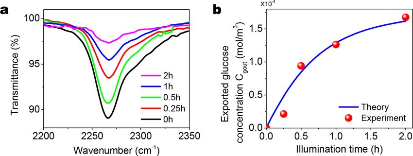
K. Yu et al.                                                                       Journal of the Mechanics and Physics of Solids 151 (2021) 104382

where Nmin is the admissible smallest chain length.
    To estimate the chain number of each type of chain length per unit volume, we treat the additional crosslinking process as m steps.
In each step, a certain amount of additional crosslinking point is introduced. We employ two methods as follows.

3.2.2.1. Method 1: equal number of incremental crosslinking points. In method 1, we assume that probabilities of forming a crosslinking
on the chain with length N0 /2i and the chain with length N0 /2j are equal, where i = 0, 1, 2⋯ and j = 0,1,2⋯. Under this assumption,
the incremental additional crosslinking density for each step is equal, denoted as dna :
                 na
         dna =                                                                                                                               (23)
                 m
     In the following, we will go through each step to calculate the volume density of polymer chains with length N0 /2j and denote it as
Cj , where j = 0, 1, 2⋯. In step 1, some of the initial chains with length N0 become shorter chains with length N0 /2 after adding dna
crosslinking point if 2dna ≤ n0 . At the end of step 1, we have:
         C0 = n0 − 2dna                                                                                                                      (24)

         C1 = 4dna                                                                                                                           (25)
   In step 2, three possible routes to form the crosslinking: between two chains with length N0 , between two chains with length N0 /2,
and between a chain with length N0 and a chain with length N0 /2. The probabilities for partitioning chains with length N0 and chains
with length N0 /2 are equal. Therefore, at the end of step 2, we have:
         C0 = n0 − 2dna − 2(dna / 2)                                                                                                       (26a)

         C1 = 4dna + 4(dna / 2) − 2(dna / 2)                                                                                               (26b)

         C2 = 4(dna / 2)                                                                                                                   (26c)
    Similarly, at the end of step 3, we have:
         C0 = n0 − 2dna − 2(dna / 2) − 2(dna / 3)                                                                                          (27a)

         C1 = 4dna + 4(dna / 2) − 2(dna / 2) + 4(dna / 3) − 2(dna / 3)                                                                     (27b)

         C2 = 4(dna / 2) + 4(dna / 3) − 2(dna / 3)                                                                                         (27c)

         C3 = 4(dna / 3)                                                                                                                   (27d)
    Eventually, at the end of step m, we have:
                      (                  )
                           1 1         1
       C0 = n0 − 2dna 1 + + + ⋯ +                                                                                                          (28a)
                           2 3         m
                         (              )
                             1 1      1
         C1 = 2dna + 2dna 1 + + + ⋯ +                                                                                                      (28b)
                             2 3      m
                                  (         )
                                   1 1    1
         C2 = 2(dna / 2) + 2dna     + +⋯+                                                                                                  (28c)
                                   2 3    m
    ……
                                  (                )
                                      1   1      1
         Cj = 2(dna / j) + 2dna         +   +⋯ +                                                                                           (28d)
                                      j j+1      m
    ……
         Cm = 4(dna / m)                                                                                                                   (28e)

    The volume density of chains with length N0 /2j at the end of step m can be summarized as
                        (                  )
                    2na      1 1         1
               n0 −       1+ + +⋯+           , j=0
                     m       2 3         m
                 (                 )
             2n 2        1       1
       Cj = { a     +       +⋯+      , 1 ≤ j ≤ m − 1 (if m ≥ 2)                                                                              (29)
              m j j+1            m
                                  4na
                                      , j=m
                                  m2

                                                                         10
K. Yu et al. Journal of the Mechanics and Physics of Solids 151 (2021) 104382
After strengthening, the polymer chain length is inhomogeneous with a chain length distribution over length of N0 , N0 /2, …., and
N0 /2m , where m ≥ 1. The chain length distribution is shown in Eq. (29). We assume that under deformation, each polymer chain
deform following an affine deformation assumption that the microscopic polymer chain deformation affinely follows the macroscopic
deformation in three principal directions; thus, the chain stretch of the chain with length N0 /2j (j = 0, 1, 2⋯) can be expressed as
(Wang and Gao, 2016; Wang et al., 2017, 2015; Xin et al., 2019; Yu et al., 2020b, 2018, 2019a)
√̅̅̅̅̅̅̅̅̅̅̅̅̅̅̅̅̅̅̅̅̅̅̅̅
Λj = λ21 + λ22 + λ23 (30)
The strain energy of the whole polymer network per unit volume can be formulated as (Wang and Gao, 2016; Wang et al., 2017,
2015; Xin et al., 2019; Yu et al., 2020b, 2018, 2019a)
∑ m [ ( )( )]
N0 βj βj
Ws = Cj kB T j + ln (31)
j=0
2 tanhβj sinhβj
( )
Λj
βj = L− 1
√̅̅̅̅̅̅̅̅̅̅̅
/ ̅ (32)
N0 2j
1/2
where the chain stretch Λj is given in Eq. (30). Under uniaxial tension with λ1 = λ and λ2 = λ3 = λ− , the tensile nominal stress of the
incompressible polymer after strengthening can be calculated as
[ (√̅̅̅̅̅̅̅̅̅̅̅̅̅̅̅̅̅̅̅)]
∑m √̅̅̅̅̅̅̅̅̅̅̅
/ ̅ λ − λ− 2 λ2 + 2λ− 1
ss1 = Cj k B T N0 2 j √̅̅̅̅̅̅̅̅̅̅̅̅̅̅̅̅̅̅̅L− 1
/ (33)
j=0 λ2 + 2λ− 1 N0 2j
In method 1, there is a hidden requirement for the relationship between na and m. For example, if m = 1, the maximal possible
crosslinking point density is n0 /2. This condition is to ensure the chain density of chains with length N0 is not negative. For a certain m,
the requirement of the possible crosslinking point density is
/[ ( )]〈 / /[ ( )]
1 1 1 1 1 1
(m − 1) 2 1+ + +⋯ + na n0 ≤ m 2 1+ + +⋯ + (34)
2 3 m− 1 2 3 m
3.2.2.2. Method 2: unequal number of incremental crosslinking points. In method 2, we assume that the probability of forming a
crosslinking on the chain with length N0 /2i is higher than that of forming a crosslinking on the chain with length N0 /2j when i < j. In
an extreme case, the crosslinking occurs first on the chain with length N0 /2i , and then on the chain with length N0 /2i+1 . In other
words, the crosslinking reaction on the longer chains always happens before the crosslinking reaction on the short chains. Following
the assumption, we can naturally define the ith step as the step with the occurrence of the crosslinking reaction on the chain with
length N0 /2i− 1 . The process will move to the next step only when there are enough crosslinkers to consume all the chains with length
N0 /2i− 1 .
If the crosslinking reaction stops at step 1, there are only two types of chains: chains with length N0 and N0 /2. Their volume
densities can be calculated as
C0 = n0 − 2na (35a)
C1 = 4na (35b)
The requirement is 0 < na /n0 ≤ 1/2.
If the crosslinking reaction stops at step 2, there are only two types of chains: chains with length N0 /2 and N0 /22 . Their volume
densities can be calculated as
( n0 )
C1 = 2n0 − 2 na − = 3n0 − 2na (36a)
2
( n0 )
C2 = 4 na − (36b)
2
The requirement is 1/2 < na /n0 ≤ 3/2.
If the crosslinking reaction stops at step m, at the end of step m, there are only two types of chains: chains with lengths N0 /2m− 1 and
N0 /2m . Their volume densities can be calculated as
[ ( ) ]
1
Cm− 1 = 2m− 1 n0 − 2 na − 2m− 2 − n0 = (2m − 1)n0 − 2na (37a)
2
[ ( ) ] ( )
1 1
Cm = 4 na − 2m− 2 − n0 = 4na − 4 2m− 2 − n0 (37b)
2 2
11K. Yu et al. Journal of the Mechanics and Physics of Solids 151 (2021) 104382
The requirement is for the additional crosslink density to reach step m is
/
2m− 1 − 1 2m − 1
< na n0 ≤ (38)
2 2
After strengthening, the strain energy function can be formulated as (Wang and Gao, 2016; Wang et al., 2017, 2015; Xin et al.,
2019; Yu et al., 2020b, 2018, 2019a)
∑m [ ( )( )]
N0 βj βj
Ws = Cj k B T j + ln (39)
j=m− 1
2 tanhβj sinhβj
( )
Λj
βj = L− 1
√̅̅̅̅̅̅̅̅̅̅̅
/ ̅ (40)
N0 2j
where the chain stretch Λj is given in Eq. (30) and Cj for j = m − 1 and j = m are given in Eq. (37). Under uniaxial tension with λ1 = λ
and λ2 = λ3 = λ− 1/2 , the nominal tensile stress of the incompressible polymer after strengthening can be calculated as
[ (√̅̅̅̅̅̅̅̅̅̅̅̅̅̅̅̅̅̅̅)]
∑m √̅̅̅̅̅̅̅̅̅̅̅
/ ̅ λ − λ− 2 λ2 + 2λ− 1
ss1 = Cj kB T N0 2j √̅̅̅̅̅̅̅̅̅̅̅̅̅̅̅̅̅̅̅L− 1 / (41)
j=m− 1
2
λ + 2λ − 1 N0 2j
4. Results
In this section, we first present the theoretical results calculated from the theory for glucose production and exportation (Section
4.1) and then from the theory for polymer strengthening by additional crosslinks (Section 4.2). In Section 4.3, we will integrate two
parts of the theories and discuss the results for glucose-enabled additional crosslinks in the polymer matrix. By coupling the photo
synthesis theory in Section 3.1 and the strengthening model in Section 3.2, we examine the effects of the illumination period, the
Table 1
Definition, value, and estimation source of the employed parameters. The estimation source is given for each parameter. I0 , η, and t are directly from
experiments. N0 and n0 is estimated based on the stress-strain behaviors of the polymer.
Parameter Definition Fig. 6 Fig. 7,8 Fig. 9 Fig. 10, Fig. 12 Fig. 13 Estimation source
11
I0 (J s− 1
m− 2 ) Initial light intensity 69.3 N/A N/A 69.3 69.3 0–69.3 Experimental data
α1 (m ) − 1 Light absorption coefficient of 2000 N/A N/A 2000 2000 2000 (Vogelmann and Evans,
the chloroplast 2002)
η (%) Mass concentration of the 5 N/A N/A 5 0–5 5 Experimental data
chloroplast
εc (%) Photosynthetic energy 5 N/A N/A 5 5 5 (Bugbee and Salisbury,
conversion efficiency of photon 1988; Zhu et al., 2010)
energy
α2 (m2 mol− 1 ) Molar absorptivity of 1 × N/A N/A 1 × 10³ 1 × 10³ 1 × 10³ (Ergun et al., 2004)
chlorophyll 103
k 1 ( s− 1 ) Reaction rate to produce proton 1 × N/A N/A 1 × 10⁴ 1 × 10⁴ 1 × 10⁴ (Lei et al., 2007)
104
kcat1 ( s− 1 ) Catalytic rate of RuBisCO 3.13 N/A N/A 3.13 3.13 3.13 (Flamholz et al., 2019;
Kubien et al., 2008)
CRubisCO (mol m − 3
) Concentration of RuBisCO 0.008 N/A N/A 0.008 0.008 0.008 (Kubien et al., 2008)
kM1 (mol m− 3 ) Michaelis constant of RuBisCO 0.0021 N/A N/A 0.0021 0.0021 0.0021 (Kubien et al., 2008)
k t ( s− 1 ) Termination rate of the starch 0.0004 N/A N/A 0.0004 0.0004 0.0004 Fitting parameter
synthesis
k d ( s− 1 ) Degradation rate of starch 0.003 N/A N/A 0.003 0.003 0.003 (Lu et al., 2005)
kcat2 ( s− 1 ) Catalytic rate of glucose 240.28 N/A N/A 240.28 240.28 240.28 (Nag et al., 2011)
transport
Ctrans (mol m− 3 ) Concentration of transportation 0.02 N/A N/A 0.02 0.02 0.02 (Nag et al., 2011)
enzyme
kM2 (mol m− 3 ) Michaelis constant of enzyme 19.3 N/A N/A 19.3 19.3 19.3 (Nag et al., 2011)
N0 Initial chain length N/A 100 40–2000 400 400 400 Chosen based on the
material
n0 (m− 3 ) Initial chain number density N/A 4.5 × 4.5 × 4.5 × 4.5 × 4.5 × Chosen based on the
1019 1019 1019 1019 1019 material
na /n0 Normalized additional crosslink N/A 0–5 2.5 N/A N/A N/A Chosen based on the
density material
t (h) Illumination time 2 N/A N/A 0–2 4 4 Experimental data
12K. Yu et al. Journal of the Mechanics and Physics of Solids 151 (2021) 104382
concentration of chloroplasts, and the light intensity on the strengthening performance. The theoretical results are compared with the
experimental results. All used parameters are presented in Table 1.
4.1. Results of part 1 theory
In Section 3.1, a theoretical framework for the production and exportation of glucose was presented. During the illumination
period, light intensity attenuates following the Beer-Lambert law (Eq. (3)). Considering a relatively thin sample (H ∼ 2 mm), we can
calculate the mean light intensity across the thickness, written as,
I0
I≈ [1 + exp(− AH)] (42)
2
where H is the sample thickness. Note that in a real situation the light intensity is inhomogeneous across the thickness: more protons
are produced at the locations closer to the light incident surface. It means that the glucose production and additional crosslinks will
vary across the interface in the later process. Since the sample is thin (i.e., 2 mm), we here simplify the problem by considering an
effectively homogeneous strengthening across the thickness. Using Eq. (42) and integrating Eq. (7), we obtain the governing equation
for the production of protons, expressed as,
∂2 CH+ 1 I
= k1 εc ηM α2 (43)
∂t2 Na hc/λ
Coupling Eqs. (43) and (10), we can calculate the concentration of the produced C6 H12 O6 in the form of starch (Cstarch
C6 H12 O6 ). A typical
curve for the production of C6 H12 O6 is shown in Fig. 6a. During the illumination period (2 h), the concentration of the produced
C6 H12 O6 in the form of starch increases over time and gradually reaches a plateau if the illumination time is long enough (Fig. 6a). The
plateau is determined by the termination of the starch synthesis which is governed by the self-metabolism of the chloroplast.
During the darkness period, the starch begins to break down to form small glucose molecules which are then exported to the
polymer matrix. Since the glucose exportation speed is dependent on the concentration of glucose within the chloroplast (Eq. (13)), the
starch breaking-down and the glucose exportation are strongly coupled. Coupling Eqs. (12)-(15), we can compute the evolution of the
starch breaking-down and the glucose exportation, which are shown in Figs. 6a and 6b, respectively. As shown in Figs. 6a, the starch
rapidly breaks down within 0.5 h. All of the produced C6 H12 O6 molecules within chloroplasts are exported to the polymer matrix (as
glucose molecules); thus, the concentration of the exported glucose increases over time and then reaches a plateau (Fig. 6b).
Fig. 6. (a) The evolution of C6 H12 O6 concentration in the form of synthesized starch in the chloroplast and (b) the evolution of the concentration of
the exported glucose in the matrix over the illumination period (2 h) and the darkness period (2 h).
13K. Yu et al. Journal of the Mechanics and Physics of Solids 151 (2021) 104382
4.2. Results of part 2 theory
We consider the polymer strengthening via forming additional crosslinks in the polymer matrix. To estimate the chain number of
each type of chain length per unit volume, we employ two methods to calculate the amount of additional crosslinking in each
crosslinking step in Section 3.2.2. As shown in Figs. 7ab and 7 cd, the polymer with initial chain length N0 = 100 becomes stronger
with increasing additional crosslinks for both method 1 and method 2. We here define the strengthening factor as the strengthened
Young’s modulus (within 10% strain region) normalized by the non-strengthened Young’s modulus (Figs. 7bd).
When the additional crosslinks density is low (e.g. na /n0 ≤ 1/2), there is only one-step strengthening in either method 1 or method
2, i.e., m = 1 (Figs. 7ac, red and green lines, Figs. 7bd). The strengthening behavior and factor show the same results by both methods.
When the additional crosslinks density is slightly larger than 1/2 (e.g. na /n0 = 0.75), the stress-strain curve and the strengthening
factor calculated from method 1 and 2 are still similar (Figs. 7ac, blue line, Figs. 7bd). However, when na /n0 increases to 1, the stress-
strain curve and strengthening factor calculated from method 1 are much larger than those calculated from method 2 (Figs. 7ac,
magenta line, Figs. 7bd). This is because the step number of method 1 reaches a larger number (m = 5) than the step number of method
2 (m = 2), corresponding to shorter chains in the polymer matrix according to Eqs. (29), (33), and (37).
To investigate the relationships between additional crosslinks density na /n0 and the step number m, we calculate the step numbers
for method 1 and 2 with na /n0 from 0 to 5 (Fig. 8). When na /n0 ≤ 1/2, the step numbers m for methods 1 and 2 are both in the first step
strengthening thus m values are the same. When na /n0 increases to 5, the step number m for method 1 drastically increases to 45.
However, the step number m is still 4 when na /n0 = 5 for method 2.
To further investigate the effect of large step numbers on the polymer strengthening, we take a relatively large crosslinking number
as an example (e.g., na /n0 = 2.5). When na /n0 = 2.5, the step number for method 1 increases to 21 (Fig. 8a), which means that the
shortest chain length in the polymer matrix becomes N0 /221 . This value should be constrained by the admissible smallest chain length
Nmin and the initial chain length N0 of the polymer in Eq. (22). Considering the stress-strain curve shape of the studied polymer
(Fig. 2), the initial chain length N0 is estimated between 60 and 2000. N0 /221 becomes an invalid number for the chain length.
Therefore, under such a situation that additional crosslink density is relatively large, method 1 cannot effectively model the
strengthening behavior, and we can only employ method 2.
Using method 2, we study the effect of the initial chain length N0 of the polymer on the strengthening effect (Fig. 9). When the
initial chain length N0 is very small (e.g. N0 = 40), the polymer can be significantly strengthened. When the initial chain length N0
Fig. 7. Theoretical results for various normalized additional crosslink density na /n0 . (a) Nominal tensile stress-strain curves for method 1. (b)
Strengthening factor in a function of the normalized additional crosslink density for method 1. The strengthening factor is defined as the
strengthened Young’s modulus normalized by the unstrengthened Young’s modulus. (c) Nominal tensile stress-strain curves for method 2. (d)
Strengthening factor in a function of the normalized additional crosslink density for method 2.
14K. Yu et al. Journal of the Mechanics and Physics of Solids 151 (2021) 104382
Fig. 8. Relationships between the step number m and additional crosslink density na /n0 for (a) method 1 and (b) method 2.
> 500, the strengthening factor reaches a plateau of around 6 (Figs. 9ab). When the initial chain length 60 ≤ N0 ≤ 2000, the
strengthening factor varies from 6 to 7.9.
4.3. Results of the integrated theory
Integrating Part 1 and Part 2 theories, we can link the experimental conditions, such as light illumination and chloroplast con
centration, to the resulting polymer strengthening. The connection between the Part 1 theory and Part 2 theory is the relationship
between the concentration of the exported glucose and the concentration of additional crosslinks. We assume that all the exported
glucose molecules are consumed by forming additional crosslinks, because the concentration of the NCO group is high enough. In
addition, as a starting point, we assume one glucose molecule only bridges two NCO groups to form one additional crosslink, that is,
na = ng = Cgout NA (44)
Eq. (44) constructs the connections between Part 1 theory and Part 2 theory. The concentration of the exported glucose calculated
in Part 1 theory can be directly passed to Part 2 theory to determine the strengthening effect.
In the following sub-sections, we will first verify our theory for the glucose production/exportation with experimental results
(Section 4.3.1), and then discuss the effects of the illumination period, the concentration of chloroplasts, and the light intensity on the
polymer strengthening (Sections 4.3.2-4).
4.3.1. Verify the theory of glucose production via experiment
After the chloroplast-embedded polymer samples go through the photosynthesis process (illumination and darkness period), the
glucose will be exported from the chloroplast to the polymer matrix. Since the photosynthesis-produced glucose is expected to
consume free NCO groups to form additional crosslinks, the concentration reduction of free NCO groups can reveal the production and
exportation of glucose. To indicate the concentration of free NCO groups within the polymer matrix, we employ a Fourier transform
infrared (FTIR) spectrometer to measure the transmittance of the sample around 2260 cm− 1 that is corresponding to the NCO bond
stretching vibration (Yu et al., 2020a). We find an evident peak at 2260 cm− 1 in the initial state of the sample (Fig. 10a). After the
Fig. 9. Theoretical results for method 2 with m = 3 and na /n0 = 2.5. (a) Nominal tensile stress-strain curves and (b) strengthening factor for various
initial chain lengths N0 .
15K. Yu et al. Journal of the Mechanics and Physics of Solids 151 (2021) 104382
photosynthesis processes (illumination period and the corresponding darkness period of the same length), the peak at 2260 cm− 1
drops, indicating the reduction of the NCO concentration. With increasing illumination periods (0–2 h), the peak height drops more.
The initial concentration of NCO groups is denoted as CNCO0 , and the concentration of NCO groups after the photosynthesis process with
illumination period ti us denoted as CNCO (ti ). To quantify the concentration reduction of NCO groups, we calculate the area under the
FTIR peak (S(ti )) and normalize the area with the initial peak area at 0 h (S0 ) (Fig. 10a). We approximate the concentration ratio of
NCO groups as
CNCO (ti ) S(ti )
= (45)
C0NCO S0
Since the consumed NCO groups have reacted with glucose molecules and one glucose molecule is assumed to consume two NCO
groups, we obtain the exported glucose concentration as
( )
S(ti )
Cgout (ti ) = 2C0NCO 1 − (46)
S0
where Cgout (ti ) is the concentration of the exported glucose after the illumination period of ti and darkness period of ti , and CNCO
0 can be
calculated from the material recipe (1.75 × 10− 4 mol/m3 ). Fig. 10b shows the relationship between the exported glucose concen
tration and the illumination period. The theoretically calculated concentration of the exported glucose agrees well with the experi
mental results obtained from Eq. (46). As shown in Fig. 10b, the exported glucose concentration increases with the illumination period
and gradually approaches a plateau when the illumination period is long enough.
4.3.2. Effect of the illumination period
With a longer illumination period, the photosynthesis process of chloroplasts is holding longer, thus leading to a higher concen
tration of produced C6H12O6 stored in the form of starch at the end of the light-dependent process (Fig. 11a). According to Eqs. (12)-
(15), the stored starch in the chloroplast will degrade to glucose molecules and then transport to the material matrix, and the glucose
molecules will serve as the additional crosslinks. With Eq. (44), the amount of the exported glucose molecules can be passed to Part 2
theory to obtain the stress-strain behaviors of the strengthened polymers with various light illumination periods (Fig. 11b). Subse
quently, Young’s moduli of the strengthened polymers can be calculated within the strain range of 10% (Fig. 11c). As the illumination
period increases, the concentration of the produced and exported glucose molecule increases, and the polymer thus becomes stiffer
with a higher Young’s modulus. As the illumination period further increases, the concentration of the exported glucose tends to
approach a plateau; thus, Young’s modulus of the strengthened polymer also tends to gradually reach a plateau (Fig. 11c). The
theoretically calculated Young’s moduli of the strengthened polymers for various illumination periods agree with the corresponding
experimental results.
4.3.3. Effect of the chloroplast concentration
The chloroplast concentration greatly influences the polymer strengthening effect (Figs. 2d-f). The effect of the chloroplast con
centration is displayed in two aspects. First, the color of chloroplast-embedded samples varies due to different concentrations of
embedded chloroplasts (Fig. 2d). Due to the color difference, the light attenuation in the material matrix depends on the concentration
of chloroplasts. This point can be modeled by Eqs. (3)-(4), where the light absorption of the material depends on the concentration of
chloroplast embedded in the polymer matrix. With increasing concentration of chloroplasts, the light intensity is attenuated more, and
thus the mean light intensity cross the thickness I is lower (Eq. (42)). Second, a higher concentration of chloroplasts (η) leads to a
higher concentration of chlorophyll (ηM in Eq. (6)), and thus more photon energy will be absorbed to produce the glucose. Since a
Fig. 10. (a) FTIR spectra of experimental group samples (with free NCO groups and embedded chloroplasts) with various light illumination periods.
The zoom-in view of FTIR spectra in the range of 2200 cm− 1 to 2350 cm− 1 indicates the concentration of the free NCO groups. (b) Experimentally
measured and theoretically calculated exported glucose concentration in a function of the illumination time. The experimental results are obtained
using Eq. (46).
16K. Yu et al. Journal of the Mechanics and Physics of Solids 151 (2021) 104382
Fig. 11. (a) The theoretically calculated C6H12O6 concentration in the form of starch for various light illumination periods. (b-c) Experimentally
measured and theoretically calculated stress-strain curves and Young’s moduli for various illumination periods. The Young’s modulus is calculated
from the stress-strain curve within 10% strain.
relatively thin sample (H ∼ 2 mm) is employed here, the effect of light attenuation is much smaller than the effect of light absorption.
Overall, with increasing concentration of chloroplasts, more C6 H12 O6 is synthesized during the light-dependent process (Fig. 12a) and
then is exported as glucose molecules in the polymer matrix. The higher concentration of the exported glucose crosslinkers then leads
to a stronger effect in the polymer strengthening. As shown in Figs. 12ab, as the concentration of chloroplasts increases from 0% to
5%, the resulting polymer matrix becomes stiffer with higher Young’s modulus. The theoretically calculated stress-strain curves and
Young’s moduli agree with the respective experimental results (Figs. 12bc).
4.3.4. Effect of light intensity
Next, we study the effect of the applied light intensity (I0 ) during the light-dependent process on the strengthening behavior.
According to Eqs. (3), (6), (42), and (43), the higher photon energy absorbed by the pigment chlorophyll induces more biomass
energy converted to generate sugars. Theoretical results show that the plateau C6 H12 O6 concentration stored in starch increases with
increasing illuminating light intensity I0 (Fig. 13a). In addition, according to Eqs. (42) and (43), such an increasing trend should be
most linear. Such a linear trend is verified by the theoretically calculated relationship between Young’s modulus of the strengthened
polymer and the applied light intensity I0 (Fig. 13b). The theoretically calculated Young’s moduli agree well with the experimentally
measured results (Fig. 13b).
Concluding remarks
In summary, we presented experiments and theories to study plant-inspired photosynthesis-assisted strengthening behaviors in a
synthetic polymer. The strengthening mechanism relies on an additional crosslinking reaction between the photosynthesis-produced
glucose and side groups within the polymer matrix. We develop a theoretical framework to explain glucose production and expor
tation, and the corresponding polymer strengthening by forming additional crosslinks. The theoretical framework can quantitatively
explain the experimentally observed photosynthesis-assisted polymer strengthening under different experimental conditions, such as
various illumination periods, concentrations of embedded chloroplasts, and light intensities.
The theoretical framework makes two significant advances in the field of solid mechanics. First, it, for the first time, proposes a
simple and easy-to-implement theory to explain the polymer strengthening effect with additional crosslinks. This framework paves the
way for the future mechanistic understanding of polymer network behaviors with incremental crosslinks, such as sequential cross
linking in double-network polymers/gels (Ducrot et al., 2014; Gong et al., 2003; Sun et al., 2012). Second, it, for the first time, proposes
a theoretical framework to bridge the communication between the natural photosynthesis process and synthetic polymer networks.
The communication between living photosynthesis and synthetic polymers may open doors for hybrid synthetic-living materials with
both complex microstructures and biomimetic properties. The theoretical framework proposed in this paper may facilitate the
mechanistic understanding of future hybrid synthetic-living materials.
Of course, the theoretical framework in this paper has been significantly simplified in multiple aspects. These aspects may forecast
future research opportunities. For example, to capture the essence of the theory, we only focus our attention on the stress-strain
behaviors within 20% strain and the corresponding Young’s modulus (Figs. 11–13), but do not fully capture the stress-strain be
haviors of the polymers until breaking during the tensile tests. As shown in Fig. 2, the stress-strain behaviors of the full strain regions
until breaking may involve chain alternation and reorganization that may lead to softening or stiffening (Wang and Gao, 2016; Wang
et al., 2015; Yu et al., 2018).
In addition, we do not consider the saturation of Young’s modulus over various chloroplast concentrations and light intensities. In
Fig. 12, we show that Young’s modulus increases with increasing chloroplast concentration within 0–5%. With further increasing
chloroplast concentration, we expect the modulus to saturate somewhere because chloroplasts that effectively behave like soft fillers
may compromise the material stiffness. In Fig. 13, we show that Young’s modulus increases linearly with the light intensity within 0 −
69.3 W/m3 . With further increasing light intensity, we expect the modulus to saturate somewhere because strong light may damage
17You can also read