Low methane emissions from a boreal wetland constructed on oil sand mine tailings
←
→
Page content transcription
If your browser does not render page correctly, please read the page content below
Biogeosciences, 17, 667–682, 2020
https://doi.org/10.5194/bg-17-667-2020
© Author(s) 2020. This work is distributed under
the Creative Commons Attribution 4.0 License.

Low methane emissions from a boreal wetland constructed
on oil sand mine tailings
M. Graham Clark1,2 , Elyn R. Humphreys1 , and Sean K. Carey2
1 Department   of Geography and Environmental Studies, Carleton University, Ottawa, Ontario, K1S 5B6, Canada
2 School   of Geography and Earth Sciences, McMaster University, Hamilton, Ontario, L8S 4L8, Canada

Correspondence: M. Graham Clark (dr.mg.clark@gmail.com)

Received: 4 July 2019 – Discussion started: 19 August 2019
Revised: 5 December 2019 – Accepted: 7 January 2020 – Published: 10 February 2020

Abstract. A 58 ha mixed upland and lowland boreal plains          1   Introduction
watershed called the Sandhill Fen Watershed was constructed
between 2008 and 2012. In the years following wetting
in 2013, methane emissions were measured using manual             The boreal biome stores large quantities of soil carbon (C)
chambers. The presence of vegetation with aerenchymous            due to the high density of peatlands with some estimates as
tissues and saturated soils were important factors influencing    high as 165 kg C m−2 (Beilman et al., 2008). A legacy of
the spatial variability of methane emissions across the con-      open pit oil sands mining in northern Alberta, Canada, will be
structed watershed. Nevertheless, median methane emissions        that almost 5000 km2 of the boreal landscape (Alberta Gov-
were equal to or less than 0.51 mg CH4 m−2 h−1 even from          ernment, 2017) will require reclamation to restore it to the
the saturated organic soils in the lowlands. Although overall     “equivalent capability” of the pre-mining ecosystems (En-
methane emissions remained low, observations of methane           vironmental Protection and Enhancement Act, 2017). These
ebullition increased over the 3 study years. Ebullition events    engineered landscapes will be important in determining the
occurred in 10 % of measurements in 2013, increasing to           long-term C footprint of the region, potentially helping to
21 % and 27 % of measurements in 2014 and 2015, respec-           offset ecological losses and industrial emissions. Rooney
tively, at the plots with saturated soils. Increasing metal ion   et al. (2012) used land cover classification and reclamation
availability and decreasing sulfur availability was measured      plans to estimate a potential net loss of 11.4–47.3 Tg of the
using buried ion exchange resins at both seasonal and an-         stored soil C from the pre-mining landscape and a reduction
nual timescales potentially as a result of microbial reduction    in CO2 sequestration capacity of the new constructed land-
of these ions. Using principle component analysis, methane        scape by 5.7–7.2 Gg C yr−1 . This loss is expected to occur
fluxes had a significant positive correlation to the leading      as a result of both the decomposition of peat when it is used
principle component which was associated with increasing          in the reclamation of uplands and from the diminished C se-
ammonium, iron, and manganese and decreasing sulfur avail-        questration capacity of engineered landscapes. In particular,
ability (r = 0.31, p < 0.001). These results suggest that an      Rooney et al. (2012) predicted that an insufficient proportion
abundance of alternative inorganic electron acceptors may be      of the disturbed area will be replaced with the C sequestra-
limiting methanogenesis at this time.                             tion capacity of the original boreal wetlands. However, wet-
                                                                  land reclamation in the region is still quite novel, and little is
                                                                  known about the surface–atmosphere exchange of C in these
                                                                  newly engineered wetlands (Nwaishi et al., 2015; Clark et
                                                                  al., 2019).
                                                                     Undisturbed peatlands are long-term CO2 sinks, accumu-
                                                                  lating C as peat over millennia (Rydin and Jeglum, 2006;
                                                                  Vasander and Kettunen, 2006). Yet, on annual timescales
                                                                  the C cycling within peatlands is highly variable and only

Published by Copernicus Publications on behalf of the European Geosciences Union.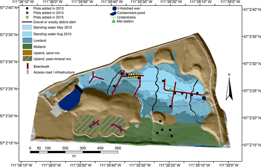
668              M. G. Clark et al.: Low methane emissions from a boreal wetland constructed on oil sand mine tailings

partially understood, particularly with regards to methane         mary productivity is positively correlated with CH4 produc-
(CH4 ) emissions (Vasander and Kettunen, 2006). Wetland            tion (Dacey et al., 1994; Megonigal and Schlesinger, 1997;
CH4 emissions are thought to be the single greatest driver         Vann and Megonigal, 2003; e.g. Whiting and Chanton, 1993;
of inter-annual variability in atmospheric CH4 concentra-          Ziska et al., 1998). Numerous studies have also shown CH4
tion (Bousquet et al., 2006), and globally wetlands are the        emissions increase in warmer soils (Bubier et al., 2005; Bu-
largest non-anthropogenic source of CH4 to the atmosphere          bier and Moore, 1994; Roulet et al., 1992; Whalen, 2005;
(Kirschke et al., 2013). Atmospheric CH4 has 28–34 times           Whiting and Chanton, 1993), although this effect may be
the global warming potential of CO2 over a 100-year time           masked when water table or other environmental factors co-
period but with a perturbation lifetime of 12.4 years in the       vary (Moore et al., 2011).
atmosphere, and its radiative forcing is much greater on              Although constructed peatlands are relatively novel,
decadal timescales (IPCC, 2013). Therefore, CH4 production         restoration of peatlands has occurred for decades by rewet-
and release is an important land–atmosphere climate change         ting drained peat, often by blocking the ditches originally
feedback process (Kirschke et al., 2013). Since methanogen-        used to drain them (Rochefort and Lode, 2006). In a compre-
esis is only favoured at the lowest reduction–oxidation (RE-       hensive review of the literature, the IPCC suggested that CH4
DOX) potentials known to support life, the high rates of CH4       emission rates from rewetted boreal sites with rich organic
emission and low rates of C turnover in peatlands are linked       soils can be estimated as 2.1 mg CH4 m−2 h−1 but encourage
to a scarcity of inorganic electron acceptors in anoxic, sat-      site-specific study because the range in the published litera-
urated soils (Hahn-Schöfl et al., 2011; Peters and Conrad,         ture is very large and not normally distributed (IPCC, 2014).
1995; Thomas et al., 2009). Around the time that Rooney            A follow-up review of the literature by Wilson et al. (2016)
et al. (2012) estimated the C balance for the post-mining          provided additional evidence that CH4 emissions were 1.7
landscapes of Alberta, the first two large-scale wetlands were     to 22.6 times greater for rewetted vs. drained boreal organic
being constructed in the Fort McMurray region. These wet-          soils. The data examined by Wilson et al. (2016) were extrap-
lands were designed and constructed to test theories on how        olated using models of average area (to include multiple sur-
to return the peat-forming and C-capturing capacities to the       face types) and annual rates, to conform with IPCC reporting
mined landscape (Wytrykush et al., 2012). A research gap           standards. Our review of paired studies which directly com-
exists, however, between the modelled predictions of C cy-         pare rewetted and drained environments shows that rewetted
cling by Rooney et al. (2012) and the actual C cycling of con-     boreal and temperate organic soils have an average of 23 and
structed wetlands. Clark et al. (2019) discussed the increas-      64 times the CH4 emissions of their drained counterparts, re-
ing CO2 sink strength over the first 3 years of one of these       spectively (Table S1 in the Supplement). However these dif-
wetlands but did not address emissions of CH4 , which can          ferences in CH4 emissions are highly variable and some stud-
contribute substantially towards the long-term C balance of        ies show a decrease in CH4 emissions after wetting (Christen
some ecosystems (Vasander and Kettunen, 2006). The aim of          et al., 2016; Juottonen et al., 2012; Urbanová et al., 2012;
this study is to evaluate CH4 emissions from this constructed      Waddington and Day, 2007). The few studies which com-
ecosystem and identify the factors which influence their tem-      pare emissions from rewetted and undisturbed wetlands (Ta-
poral and spatial variability.                                     ble S1) show a wide range of results with rewetted wetland
   Methane emissions from wetlands are highly variable in          emissions < 1 % (Juottonen et al., 2012), 19 % (Beetz et al.,
space and time (Moore et al., 1998). Four key wetland char-        2013), 43 % (Urbanová et al., 2012), and 127 % (Christen et
acteristics are typically linked to the temporal and spatial       al., 2016) of the emissions observed in undisturbed wetlands.
variability of CH4 flux in peatlands: water table position, RE-       To determine the CH4 emissions of a closure watershed
DOX, vegetation composition, and temperature (Ding et al.,         in the oil sands mining region of northern Alberta and how
2005; Kim et al., 2012; Limpens et al., 2008; Turetsky et al.,     these emissions compare to those from the restored peat-
2014; Vasander and Kettunen, 2006). Approximately 60 % to          lands listed above, this paper presents 3 years (2013–2015)
90 % of the CH4 produced in peatlands is reoxidized before         of CH4 emission measurements from the Sandhill Fen Water-
it reaches the atmosphere (Le Mer and Roger, 2001). Emis-          shed (SFW), one of the first wetland complexes constructed
sions tend to be higher in areas with a high water table as this   in the Athabasca oil sands region (AOSR). Once water was
limits the potential for CH4 oxidation (Moore et al., 2011),       added to the SFW, approximately 17 ha of the 58 ha construc-
while deep rooting vegetation with aerenchymatous tissues          tion had permanently saturated peat soils with little horizon-
(Couwenberg, 2009; Kludze et al., 1993) allow CH4 to by-           tal or vertical water flow (Nicholls et al., 2016) and thriving
pass the aerated surface peat where aerobic methanotrophic         plant communities including species with aerenchyma (e.g.
communities reside. Aerenchymatous tissues can also trans-         Carex spp.) (Vitt et al., 2016). We hypothesized that these
port oxygen into the rhizosphere, which can increase RE-           areas would be a significant source of CH4 and these CH4
DOX potentials and create unfavourable niches for anaero-          emissions would be an important component of the C bal-
bic microbial communities (Blossfeld et al., 2011). Rhizo-         ance of the SFW. Results of this research will provide im-
spheric microbial communities readily metabolize the labile        portant information on the greenhouse gas and C budget for
organic compounds exuded by roots such that plant net pri-

Biogeosciences, 17, 667–682, 2020                                                        www.biogeosciences.net/17/667/2020/
M. G. Clark et al.: Low methane emissions from a boreal wetland constructed on oil sand mine tailings                       669

reclamation ecosystems in the AOSR and help guide future              In the third growing season (2015) since the ecosystem
strategies for ecosystem design and C management.                  was seeded/planted (see Vitt et al., 2016, for more details),
                                                                   there were four distinct plant communities in the lowland
                                                                   roughly distributed along a soil moisture and water depth
2   Study site                                                     gradient (Vitt et al., 2016). The areas with standing water
                                                                   (Fig. 1) were dominated by Carex aquatilis Wahlenb., Typha
The SFW (57.0403◦ N, 111.5890◦ W) was designed to re-
                                                                   latifolia L., and to a lesser extent Carex utriculata Stokes,
claim sand-capped soft tailings with the conditions needed
                                                                   while areas with the water table near the surface contained
to promote the long-term development of a peat-forming bo-
                                                                   the most species associated with peatlands including sedges
real plains ecosystem (Wytrykush et al., 2012). Details of the
                                                                   and bryophytes (Vitt et al., 2016). The drier areas contained
SFW construction were described by Wytrykush et al. (2012)
                                                                   the largest percentage of weedy species, or species not as-
and others (Biagi et al., 2019; Nicholls et al., 2016; Oswald
                                                                   sociated with peatlands (Vitt et al., 2016). The midland and
and Carey, 2016; Vitt et al., 2016). Clark et al. (2019) de-
                                                                   organic soil regions of the upland were populated by planted
scribed the three main topographic features of the SFW as
                                                                   trees (Populus tremuloides Michx., Betula papyrifera Mar-
a lowland region (the wetland), a midland region (drained
                                                                   shall, Picea glauca Monech, Picea mariana Mill., Larix lar-
but moist organic soils), and an upland region lying 2 to
                                                                   icina Du Roi, and Pinus banksiana Lamb.) and local grasses
6 m above the wetland with well-drained sandy soils and two
                                                                   (e.g. Hordeum jubatum L.) that had naturally colonized the
experimental perched wetland sites with moist organic soils
                                                                   region. Vegetation cover throughout the whole watershed in-
(Fig. 1). The sand of the lowland, midland, and perched wet-
                                                                   creased over time; peak season leaf area index increased from
land regions was covered with 0.5 to 1 m of peat coarsely
                                                                   1.5±0.6 to 2.2±1.1 over the 3 years as measured at 15 plots
mixed with some underlying mineral soil via excavation of
                                                                   (5 midland, 10 lowland) using a plant canopy analyzer (LAI-
nearby peatlands before mining. A goal of the SFW design
                                                                   2200, LI-COR Inc., Lincoln, NE).
was to limit vertical transport of tailings and process-affected
waters (i.e. water with some component of industrial wastew-
ater known to contain salts and naphthenic acids) to the sur-
                                                                   3   Materials and methods
face (Wytrykush et al., 2012). To achieve this, fine sediments
with 26.4 %–46.4 % clay (based on texture analysis) were
                                                                   This study used plot-scale measurements of CH4 fluxes
placed in the lowland regions of the SFW to help minimize
                                                                   over 3 years to assess the temporal and spatial varia-
vertical transport of process-affected waters from the tailings
                                                                   tions in CH4 emissions and the factors that influence their
below.
                                                                   variability. Fluxes were measured using non-steady-state
   Initially, freshwater was pumped into the containment
                                                                   static chambers following methods described by Wilson and
pond in the west end of the SFW in 2013 (Fig. 1). This water
                                                                   Humphreys (2010). Plots were established over the 3 years of
flowed through a leaky gravel dam into the SFW to initially
                                                                   study to sample the dominant landforms and built features of
saturate the lowland region. A downstream pump was used
                                                                   the SFW. In 2013, 15 plots were established across the low-
to remove water from an outlet V-notched weir (Fig. 1). Ex-
                                                                   land and midland of the SFW. In 2014, the number of plots
cept for a few hours of operation, the pumps were not used in
                                                                   was increased to 21 by including plots on the organic soils
2014 or 2015. Four underdrains, which run along the central
                                                                   in the perched wetlands (upland region) and in 2015 was in-
area of the lowland region, were placed to limit the upwelling
                                                                   creased to 29 by adding more plots in the lowland (Fig. 1).
of the salt-rich process water. The underdrains were not op-
                                                                   The 2013 plots were chosen before the pumps were activated
erated after the beginning of the 2014 growing season.
                                                                   and were selected to capture the surface moisture and vegeta-
   After placement and before wetting, the top 0.25 m of
                                                                   tion heterogeneity while maintaining multiple plots on simi-
the donor peat/mineral material in the midland and low-
                                                                   lar landforms. The midland plots were chosen to capture dif-
land had a mean (± SD) C-to-nitrogen (N) ratio of 22.7
                                                                   ferences in the vegetative cover. Two plots were placed on
(±3.4), N content was 0.98 (±0.36) % by dry weight, Ca
                                                                   sandy soils, one directly on exposed tailings sand and the
and Na concentrations were 786.1 (±409.4) and 184.2
                                                                   other on the salvaged mineral soil mixture. In 2014, the new
(±79.0) mg kg−1 , respectively, and electrical conductivity
                                                                   collars were placed on the experimental wetland sites that
was 1980 (±600) µS cm−1 (n = 107). The concentration of
                                                                   were depressions built into the upland hills. Note that these
Fe was 8028 (±2712, n = 13) mg kg−1 and SO2−           4    con-
                                                                   upland plots remained moist but well drained for the duration
centration was high, with a mean of 914.0 (±425.5, n =
                                                                   of the measurements. The eight new collars in the lowland
107) mg S kg−1 . Total S concentration by dry weight was
                                                                   added in 2015 were placed along a moisture gradient tran-
also high at 1.00 % (±0.50 %, n = 12) determined by ox-
                                                                   sect also used for REDOX monitoring (described below).
idation in an induction furnace then quantified through in-
                                                                      The midland plots had water table depths over 0.5 m be-
frared mass spectroscopy with a LECO IR (LECO Corpora-
                                                                   low the surface and all upland plots had water table depths
tion, Saint Joseph, MI).
                                                                   exceeding 1 m. For the remainder of this paper, midland and
                                                                   upland plots were combined into one group called “upland”

www.biogeosciences.net/17/667/2020/                                                        Biogeosciences, 17, 667–682, 2020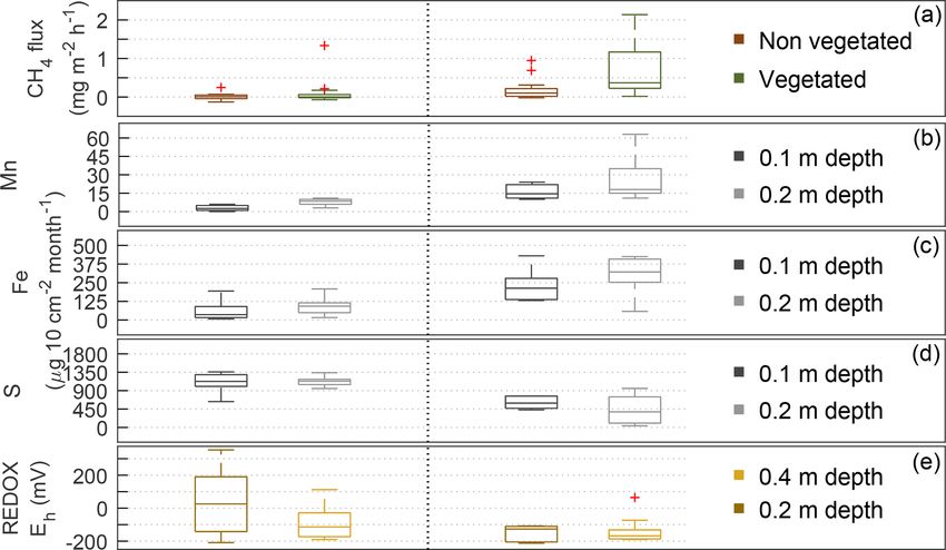
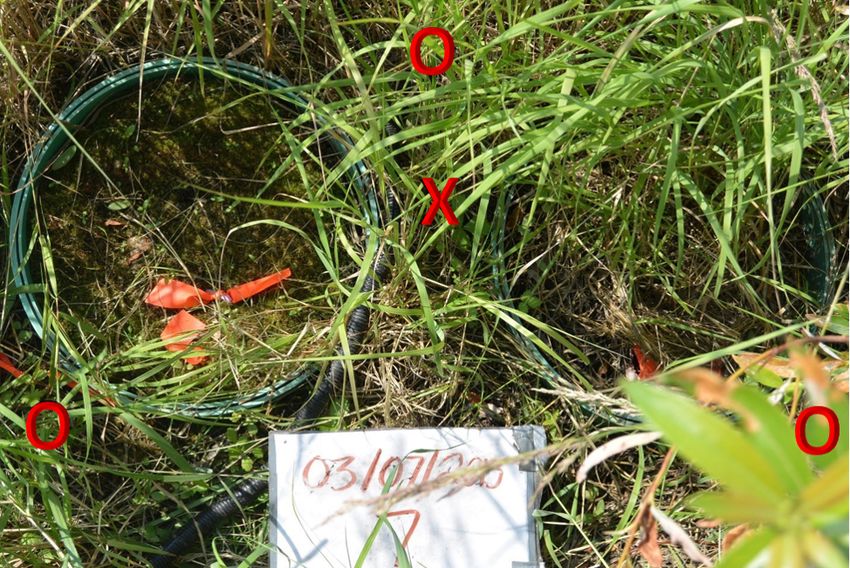
670              M. G. Clark et al.: Low methane emissions from a boreal wetland constructed on oil sand mine tailings

Figure 1. Map of the Sandhill Fen Watershed. Standing water was limited to the lowland region only.

due to their similar soil, water table depth, and vegetation          tained equal pressure with the surroundings (Hutchinson and
characteristics. In the lowland, the “saturated” plots were           Livingston, 2001). During a measurement, the air inside the
those with volumetric soil water content ≥ 86 % (i.e. fully           chamber was mixed by pumping a 60 mL syringe connected
saturated), and all remaining plots were part of the “unsat-          to the chamber sampling line and then pulling 24 mL of air
urated” group. Only five lowland plots switched categories            from the chamber volume at 0, 5, 10, 15, and 20 min inter-
in 2013 and early spring 2014 and 2015, all periods when              vals. The sampled air was injected into a 12 mL evacuated
CH4 emissions were uniformly low with no discernible dif-             vial containing a small amount of magnesium perchlorate to
ferences among the groups. Water table depth was not moni-            remove any water vapour from the air sample. Flux measure-
tored at each plot, but the soil moisture measurement method          ments were made between late May and early August in all
is described below.                                                   3 years, referred to hereafter as the growing season. The air
   Each plot included a pair of 0.19 m tall collars with a sur-       samples were transported to Carleton University where CO2
face area of 0.07 m2 that were inserted until nearly flush            and CH4 concentrations were measured on a gas chromato-
with the soil surface to minimize changes to the microcli-            graph (CP 3800, Varian, CA) within a few months of sam-
mate as a result of the collar (Parkin and Venterea, 2010).           pling. The operational details of the gas chromatograph (GC)
Each pair consisted of one collar that was maintained free            are described in Wilson and Humphreys (2010).
of vegetation by clipping and the other was left undisturbed             During the initial collar installation, five thermocouples
(Fig. 2). A limitation of the undisturbed collar was that any         were buried to a depth of 2, 5, 10, 20, and 50 cm at each
vegetation larger than the flux chambers (0.4 m tall, 0.03 m3 )       plot between the two collars. At the time chamber flux mea-
was trimmed to fit within the chamber. This trimming had              surements were made, soil temperatures were recorded from
the largest effect in the lowland, where some Typha died              the buried thermocouples. A portable soil water sensor that
once trimmed. The collars were made of SDR35 12” PVC                  integrated over the upper 0.2 m of soil (HydroSense, Camp-
sewer pipe with a groove cut into the top edge where an               bell Scientific Inc., Utah, USA) was used to measure volu-
acrylic chamber was placed during measurement. The cham-              metric water content of the soil at three locations surround-
bers were constructed of acrylic and were covered in opaque           ing each of the collars. When there was standing water over
black plastic to reduce heating within the chamber and elim-          0.05 m deep, no manual soil water measurements were made.
inate photosynthetic uptake of CO2 for a respiration analysis         In those cases, the soil moisture was estimated at 87 % (an es-
discussed by Clark et al. (2019). A seal between the cham-            timate of saturated conditions based on an average soil bulk
ber and collar was made by filling the groove with water.             density of 0.28 g cm−3 ).
A small coiled vent tube on the top of the chamber main-

Biogeosciences, 17, 667–682, 2020                                                            www.biogeosciences.net/17/667/2020/
M. G. Clark et al.: Low methane emissions from a boreal wetland constructed on oil sand mine tailings                                671

                                                                         NOS III rods (Vorenhout et al., 2011) inserted into the soil
                                                                         every 2 m alongside the 20 m transect of new plots to eval-
                                                                         uate the impacts of a moisture gradient on CH4 emissions
                                                                         (Fig. 1). The HYPNOS rods were equipped with four plat-
                                                                         inum probes and thermistor temperature sensors, of which
                                                                         the sensors 0.2 and 0.4 m below the surface were used in this
                                                                         study. The reference was a pH probe with a 0.1 M KCl stan-
                                                                         dard buried below the water table near the middle of the tran-
                                                                         sect. The probes were connected to two HYPNOS data log-
                                                                         gers and the standardized REDOX potentials (n = 36) were
                                                                         calculated as the sum of the measured potential and the refer-
                                                                         ence potential. No pH correction was applied to probe mea-
                                                                         surements because pore water remained circumneutral and
                                                                         stable throughout the season. During summer 2015, the mean
Figure 2. Example of a plot with a collar pair in the wetland area il-   pH was 7.1 ± 0.4 (± SD) as determined using weekly mea-
lustrating a collar excluding vegetation (on the left) and a vegetated   surements at a nearby pore water sampling well that inte-
collar (right) and surface PRS probes (orange and purple tabs with       grates the water from ∼ 1 m depth to the surface. Early spring
orange flagging tape; locations outside the collar are marked with       (20 May) had the largest discrepancy between the well and
circles). The permanent soil thermocouple profile post is marked by      surface water measurement locations, with the surface water
an “X”. This plot is from the lowland unsaturated category (bottom       at a pH of 7.6 and the well water at 6.2. By early July the two
of the easternmost boardwalk, Fig. 1), and the photograph was taken      sampling locations had almost converged at neutral, with a
on 3 July 2015.
                                                                         slightly higher pH in the surface water (∼ 7.4 vs. 6.9).
                                                                            Within each plot, three replicate sets of plant root simu-
                                                                         lator (PRS) probes (Western Ag., Saskatoon, Canada) were
   Fluxes in units of mg C-CH4 m−2 h−1 were calcu-                       buried at a depth of 0.1 m (shallow) and 0.2 m (deep) out-
lated from the linear rate of change in CH4 mixing ra-                   side the collars. PRS probes are ion exchange membranes
tios (nmol CH4 mol−1 air), the molar density of the air                  designed to mimic in situ soil–root exchange of nutrients
in the chamber (mol air m−3 ), the chamber volume (m3 )                  and other ions in a non-destructive manner (Qian et al.,
and area (m2 ), and the molecular weight of carbon                       2008; Qian and Schoenau, 2005). PRS probes provide a time-
(mg C nmol−1 CH4 ). To determine air density, barometric                 integrated representation of the soil nutrient availability and
pressure was recorded at a nearby micrometeorological sta-               net adsorption rates in units of ion mass per membrane area
tion (Fig. 1) and chamber temperature was estimated using                per burial time. These values differ from the more common
the 0.02 m thermocouple at each plot. The chamber volume                 point-in-time soil extraction measurements (typically ele-
was adjusted for the different collar heights and depth of               ment mass per mass of dry soil), although studies show good
standing water. All calculations and statistical analyses were           correspondence between methods for N, P, K, and S (Harri-
carried out with MATLAB 2015 (MathWorks Inc., Mas-                       son and Maynard, 2014; Qian et al., 1992). The probes were
sachusetts, USA).                                                        buried for 28 d (∼ 1 month), with three consecutive burial pe-
   The R 2 coefficient from the linear regression of CH4 con-            riods monitored each year starting on days 149, 146, and 146
centration over time is not suitable as a quality control metric         for 2013, 2014, and 2015, respectively. For simplicity, since
by itself (Lai et al., 2012). For example, when the fluxes ap-           the midpoint of each of these three 1-month burial periods
proach zero, the slope also approaches zero and small vari-              corresponds roughly to the start of June, July, and August,
ability in gas concentrations results in low R 2 values. In to-          results from each period were referred to as the result from
tal, 16 % of the fluxes had an R 2 over 0.9 % and 28 % over              those months (i.e. the July ion adsorption rate refers to the
0.8. Instead of the typical R 2 filtering, quality control of the        moles of ions absorbed by the PRS probe period between the
data was done by a visual inspection of each time series used            174th and 202nd days of the year). An example plot with
to calculate the fluxes. Any flux measurement which had a                collars, PRS probes, and thermocouples is shown in Fig. 2.
distinctly non-monotonic or non-linear trend due to individ-                Temporal trends in the PRS probe ion data were assessed
ual data point anomalies was removed from further analysis               using Spearman rank correlations using three different tem-
(6.4 %, 12.3 %, and 11.2 % of the flux measurements in 2013,             poral groupings of the data. First, the data were binned into
2014, and 2015, respectively). These anomalies included iso-             categories 1 to 9, representing each of the 3 months across 3
lated large decreases in concentration or a return to ambient            years of measurements (for example, June of the third year
concentration or isolated or unsustained large increases in              was category 7). Second, the data were binned into three cat-
concentration and represented fluxes from a leaking cham-                egories corresponding to the 3 months of measurements each
ber or an ebullition event (Tokida et al., 2007). In 2013 RE-            year, regardless of year, to ignore the inter-annual trends. Fi-
DOX potential was measured every 15 min with nine HYP-                   nally, the data were binned by year, regardless of the collec-

www.biogeosciences.net/17/667/2020/                                                                Biogeosciences, 17, 667–682, 2020
672 M. G. Clark et al.: Low methane emissions from a boreal wetland constructed on oil sand mine tailings
tion month, to ignore the monthly and seasonal trends. This erage air temperatures recorded at 3 m above the lowland
allowed some quantification of the seasonal trends relative were 16.4, 15.3, and 15.3 ◦ C and total rainfall was 375.1,
to the inter-annual trends in all three groups (upland and the 299.1, and 231.3 mm for the 2013, 2014, and 2015 growing
saturated and unsaturated lowland groups). seasons, respectively. The 1981–2010 climate normal for this
To relate CH4 fluxes, REDOX, and PRS probe results, a period was 13.3 ◦ C and 211.1 mm at a nearby weather station
principal component analysis (PCA) was performed on the (Fort McMurray Airport; 48 km from study area; Environ-
standardized measurements (z scores) of net ion adsorption ment and Climate Change Canada, 2016). Over the 3-year
rates from the PRS probes buried at 0.2 m depth in the nine study period, the upland plot soils were drier and slightly
plots with REDOX probes. The availability of alternative warmer than the lowland plots with an average volumetric
2−
electron acceptors including NH+ 4+ 3+
4 , Mn , Fe , and SO4 soil moisture of 34.7 % compared to the 57.5 % in the low-
are linked to varying soil REDOX potential through their land (Table 1). There were only small differences in grow-
participation in microbially mediated REDOX reactions. It ing season 0.02 m soil temperatures at the plot level (Ta-
should be noted that although PRS probes adsorb all mo- ble 1). Near the climate monitoring station in the centre of
bile forms of S, most are expected to be SO2− 4 (Li et al., the lowland the electrical conductivity was measured to be
2001). Using Pearson correlation, the relationship between 1171 ± 269, 2109 ± 306, and 2163 ± 248 µS cm−1 in 2013,
the leading two principal components and 0.2 m REDOX 2014, and 2015, respectively, where the typical electrical
measurements were assessed. Pearson correlation was also conductivity of boreal wetland pore waters ranges from 400
used to assess the relationship between the leading two prin- to 2770 µS cm−1 (Trites and Bayley, 2009).
cipal components and the log-transformed CH4 flux (trans-
formed to account for skew) averaged over the burial period. 4.1 Spatial and temporal CH4 and ion relationships in
Methane fluxes were increased by a common absolute value the SFW
of the minimum flux observed in the study (−0.10 mg C-
CH4 m−2 h−1 ) to permit the log transformation. Pearson cor- During each growing season, CH4 emissions were generally
relation was also used to assess any linear relationships be- very low, with median values less than or equal to 0.04 mg C-
tween the transformed CH4 flux and soil moisture and 0.02 m CH4 m−2 h−1 for all plot groups (Table 1). The greatest me-
soil temperature. Individual Pearson correlations were calcu- dian CH4 emissions were from the saturated plots (all located
lated between the mean transformed CH4 flux and the net ion in the lowland) in July 2015 with median emissions reaching
adsorption rates at the two burial depths for a burial period. 0.51 mg C-CH4 m−2 h−1 (Fig. 3).
The effects of vegetation and standing water on CH4 fluxes The proportion of measurements where substantive CH4
were evaluated using a linear mixed-effect (LME) model: emissions were detected increased for the saturated plots
over the study period (Table 1). This included occasions
methane fluxij = αij + ζ0j + β1 vegetated ij with ebullition or when fluxes were greater than 0.5 mg C-
+ β2 saturated ij + ij , (1) CH4 m−2 h−1 , which is equivalent to 10 times the maximum
CH4 uptake rate observed at this site and is in the upper range
where vegetated and saturated were binary vectors indicat- of average uptake rates observed in grassland and forest soils
ing if the measurement comes from a vegetated plot or a satu- around the world (Yu et al., 2017). Among all three groups
rated plot, respectively. i and j subscripts represent measure- and years, the 2015 saturated plots had the highest proportion
ments from each sampling day and site, respectively. β is the of CH4 emissions exceeding 0.5 mg C-CH4 m−2 h−1 (6.5 %)
slope of the fixed effect, ε the residual, α the intercept, and and the highest number of ebullition events (26.6 %). Veg-
ζ the random effect from the repeated measures occurring at etated collars had a higher median CH4 flux than in collars
each site. with vegetation excluded, particularly in the saturated plots
An independent but similar LME model was constructed (Fig. 3). There appeared to be an increase in CH4 emissions
to detect significant effects of soil depth and standing water over time in the vegetated collars within the saturated plots
on PRS net ion adsorption rates and REDOX potentials; the both within the growing season and inter-annually.
vegetated covariate was replaced with the binary vector deep, The rates of Mn2+ , Fe2+ , and NH+
which represented the relative depth of the REDOX or PRS 4 ion adsorption on the
PRS probes were greatest in the saturated lowland plots and
measurement (i.e. deep or shallow): lowest in the upland plots. By 2015, net adsorption of S was
PRS ion/REDOX potentialij = αij + ζ0j + β1 deep ij lower in the saturated lowland plots than in the upland plots
(Fig. 4). The ion with the strongest absolute temporal trend
+ β2 saturated ij + ij . (2)
in adsorption was S (Table 2, Fig. 4), with most of this trend
likely a result of changes in SO2− 4 availability (Geer and
4 Results Schoenau, 1994; Li et al., 2001). In the saturated plots, mo-
bile S decreased seasonally, annually, and over the duration
The three growing seasons (1 May through 31 September) of the study (the greatest Spearman rank coefficient was for
were warmer and wetter than the long-term average. The av- 0.25 m deep S ion adsorption rates and chronological time
Biogeosciences, 17, 667–682, 2020 www.biogeosciences.net/17/667/2020/M. G. Clark et al.: Low methane emissions from a boreal wetland constructed on oil sand mine tailings 673
Table 1. Soil and CH4 flux characteristics of the three location groups. The standard deviation from the mean is reported in brackets.
Dominant vegetation is the most common plant type among the vegetated collars (by percentage of cover).
Lowland – Lowland – Upland –
saturated unsaturated unsaturated
Number of plotsa 2013 7 4 6
2014 7 4 12
2015 9 13 12
Median CH4 flux 2013 0.00 (±0.68) 0.00 (±0.05) 0.00 (±0.06)
(mg C-CH4 m−2 h−1 ) 2014 0.02 (±0.25) 0.00 (±0.04) −0.01 (±0.06)
2015 0.04 (±0.32) 0.01 (±0.28) 0.00 (±0.15)
Maximum CH4 flux 2013 6.64 0.20 0.42
(mg C-CH4 m−2 h−1 ) 2014 2.04 0.08 0.43
2015 2.14 3.77 2.07
Proportion of flux 2013 10.0 %/2.1 % 8.0 %/0.0 % 1.6 %/0.0 %
measurements with 2014 21.4 %/2.0 % 14.5 %/0.0 % 7.7 %/0.0 %
ebullition/proportion of 2015 26.6 %/6.5 % 5.4 %/1.4 % 6.3 %/0.7 %
CH4 emissions
> 0.5 mg C-CH4 m−2 h−1
Mean 0–0.2 m 2013 87.0 (±0.4) 51.3 (±20.7) 55.1 (±34.6)
volumetric soil 2014 87.0 (±0.0) 54.2 (±12.7) 34.5 (±21.4)
moisture (%, ±1 SD)b 2015 87.0 (±0.0) 59.2 (±9.7) 29.3 (±20.4)
Mean 0.02 m soil 2013 14.4 (±7.8) 12.2 (±9.4) 17.2 (±8.4)
temperature 2014 15.9 (±9.0) 14.0 (±7.8) 19.0 (±7.0)
(◦ C, ±1 SD) 2015 14.0 (±7.7) 16.4 (±7.1) 17.0 (±6.8)
Mean sulfur 2013 1206 (±186) 1324 (±144) 828 (±534)
adsorption rates at 2014 718 (±430) 1321 (±124) 857 (±402)
PRS probes 2015 606.0 (±277.0) 1240.0 (±238.5) 907.4 (±423.2)
(µg S m−2 per month)
Number of chamber 2013 126 58 124
measurements 2014 77 71 216
2015 135 262 252
Dominant plant types 2013 Sedges, grasses Grasses, sedges, shrubs Grasses, herbs, shrubs
within the vegetated 2014 Cattails, sedges, rushes Grasses, sedges, herbs, shrubs, rushes, cattails Grasses, herbs, shrubs
collars 2015 Cattails, sedges, rushes Grasses, sedges, herbs, shrubs, rushes, cattails Grasses, herbs, shrubs
a As the water table declined, plots were reclassified as unsaturated in the lowland at the time of sampling. Therefore, the sum of the groups each year exceeds the number of
chambers reported in the text for that year. b When standing water was observed, soil moisture was not measured, and the volumetric soil moisture was set to 87 %. The depth of
standing water varied from 0.03 to 0.33 m.
represented as increasing values 1 through 9, Table 2). De- 4.2 Spatial and temporal relationships along a
clines in net S adsorption were also observed in the other plot moisture gradient in the lowland
groups but the greatest decline was in the saturated lowland
plots, where, relative to 2013 values, 2014 values were 40 % Along the moisture gradient established by a slightly sloping
lower and 2015 values were 50 % lower (Table 1 and Fig. 4). surface in the north-eastern part of the lowland (Fig. 1), CH4
Correspondingly, net adsorption rates for Mn2+ , Fe2+ , and emissions were higher in the four saturated plots than in the
NH+ 4 ions significantly increased over time at the saturated five unsaturated plots (Fig. 5). Methane emissions were also
plots (Table 2). higher in vegetated collars than in collars with vegetation
excluded. Using a LME model (Eq. 1), and controlling for
sampling location as a random effect, CH4 emissions were
0.34 ± 0.11 mg m−2 h−1 greater in saturated plots than un-
saturated plots and 0.17 ± 0.06 mg m−2 h−1 greater in veg-
etated collars than collars without vegetation over the Au-
www.biogeosciences.net/17/667/2020/ Biogeosciences, 17, 667–682, 2020674 M. G. Clark et al.: Low methane emissions from a boreal wetland constructed on oil sand mine tailings
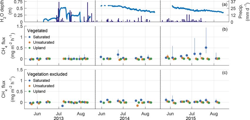
Figure 3. Water table, precipitation, and median CH4 fluxes by sampling date. Water table depth and precipitation (a) were measured at
the central meteorological station (Fig. 1). Circles indicate median CH4 flux on the day of sampling, and lines indicate the 25th to 75th
percentiles for collars with vegetation (b) and collars maintained free of vegetation (c). An offset between vegetation groups has been added
to the x axis to reduce overlapping points. All groups were sampled on the same day, roughly once a week. Tick marks on the x axis indicate
first day of the labelled month. If the upper 75th percentile exceeded the range of the y axis, the value is printed on the plot.
Table 2. Spearman rank correlations to assess temporal trends in net ion adsorption rates for the three plot groups. Plant root simulator (PRS)
data were categorized into chronological order (1–9 for the three burial periods over 3 years, “Combined”), seasonal order regardless of year
(1–3, “Seasonal”), and annual order regardless of season (1–3, “Annual”). Bold values indicate a significant trend at α = 0.01. The greatest
temporal trend across all plot groups for a given ion and depth is in italic.
Ion Lowland saturated Lowland unsaturated Upland
Combined Seasonal Annual Combined Seasonal Annual Combined Seasonal Annual
Shallow Mn2+ 0.26 0.22 0.21 −0.21 −0.29 −0.11 –0.35 −0.32 −0.23
Deep Mn2+ 0.54 0.17 0.52 0.49 0.07 0.50 −0.27 −0.29 −0.17
Shallow Fe2+ 0.47 0.48 0.37 0.26 0.06 0.29 −0.01 −0.26 0.08
Deep Fe2+ 0.64 0.34 0.60 0.54 0.26 0.52 0.07 −0.16 0.10
Shallow S –0.64 −0.45 −0.54 0.03 −0.31 0.15 −0.02 −0.08 0.05
Deep S –0.74 −0.32 −0.71 −0.43 −0.48 −0.25 −0.08 −0.20 0.03
Shallow TN −0.19 −0.10 −0.19 –0.33 −0.19 −0.22 −0.17 0.04 −0.19
Deep TN −0.05 −0.09 −0.03 –0.28 −0.02 –0.28 −0.25 −0.01 −0.25
Shallow NO−
3 –0.36 –0.36 −0.26 −0.30 −0.35 −0.10 −0.08 −0.06 −0.04
Deep NO−
3 −0.14 −0.26 −0.05 –0.35 −0.27 −0.22 −0.15 −0.04 −0.13
Shallow NH+
4 0.19 0.18 0.15 −0.14 0.17 −0.16 −0.33 0.43 –0.54
Deep NH+
4 0.21 0.25 0.16 0.21 0.38 0.08 −0.37 0.31 –0.50
gust period (Table 3), when CH4 fluxes were greatest, in both lower S net adsorption; Fig. 5). Using just the August data
magnitude and proportion of emissions exceeding 0.5 mg C- from all lowland plots, the LME model indicated that the av-
CH4 m−2 h−1 (Table 1). Temperature and soil moisture were erage net adsorption of Mn2+ was 16.0 ± 3.7 µg 10 cm−2 per
also included in an earlier version of the LME model, but month higher in saturated conditions and 7.1±2.3 µg 10 m−2
they did not have a significant effect on CH4 emissions so per month higher for the deeper (0.2 m) probes. The net ad-
were removed from the model. sorption of Fe2+ was 188 ± 36 µg 10 m−2 per month higher
When CH4 emissions were greatest in the saturated plots, in saturated conditions, but there was no significant dif-
both REDOX potential and the PRS ion adsorption rates in- ference at depth (β2 = 42 ± 24). The net adsorption of S
dicated reduced soil conditions (higher Mn2+ and Fe2+ and was 588 ± 92 µg 10 m−2 per month lower in the saturated
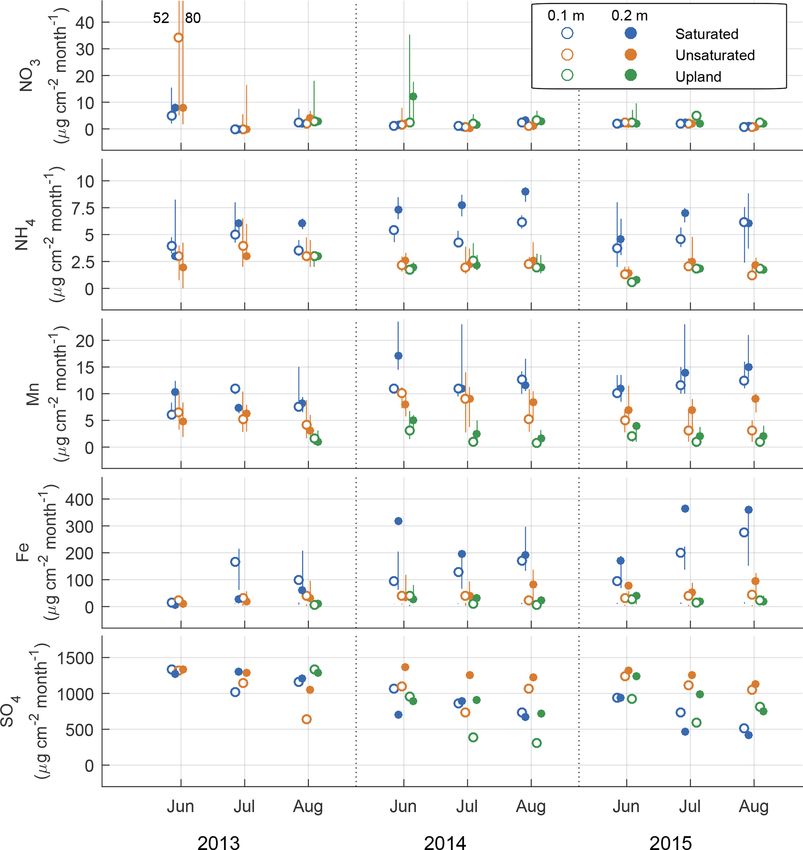
Biogeosciences, 17, 667–682, 2020 www.biogeosciences.net/17/667/2020/M. G. Clark et al.: Low methane emissions from a boreal wetland constructed on oil sand mine tailings 675 Figure 4. Ion availability as measured using plant root simulator ion exchange resins over the three monthly burial periods for 3 years expressed in units of µg 10 cm−2 per month at two depths (0.1 and 0.2 m). Units are a function of time the probes were buried for. Metal ions were measured in their reduced forms and mobile S is the oxidized form of sulfur. An offset has been added between groups on the x axis to reduce overlapping points. Table 3. Results of the linear mixed-effect models for CH4 emissions, PRS ions, and REDOX potential (Eqs. 1 and 2) measured August 2015 at the nine plots along the moisture gradient in the lowland of the Sandhill Fen Watershed. Values are the mean effect ± the standard deviation. Bold values indicate parameters significantly different from zero at the α = 0.05 level. Vegetation effects are only for the CH4 emission model (Eq. 1). Plot effect is the standard deviation of the random effects from each plot. Response F value β1 (saturated) β2 (depth/vegetation) α (intercept) Var(ζ )1/2 (plot effect) variable CH4 0.84 0.34 ± 0.11 mg m−2 h−1 0.17 ± 0.06 mg m−2 h−1 −0.04 ± 0.07 mg m−2 h−1 0.18 mg m−2 h−1 Mn2+ 3.12 16.0 ± 3.7 µg 10 cm−2 per month 7.1 ± 2.3 µg 10 cm−2 per month 1.7 ± 2.5 µg 10 cm−2 per month 5.5 µg 10 cm−2 per month Fe2+ 2.99 188 ± 36 µg 10 cm−2 per month 42 ± 24 µg 10 m−2 per month 57 ± 25 µg 10 cm−2 per month 51 µg 10 cm−2 per month S 3.8 −588 ± 92 µg 10 cm−2 per month −74 ± 62 µg 10 m−2 per month 1145 ± 64 µg 10 cm−2 per month 126 µg 10 cm−2 per month REDOX 0.42 −116 ± 47 mV −85 ± 33 mV 13 ± 32 mV 44 mV plots, but there was no significant difference between the two dard) lower in saturated conditions and 85 mV ± 33 lower at depths (β2 = −74±63). The median REDOX potentials were a 0.4 m depth (Table 3). −127 and −168 mV in the saturated plots at 0.2 and 0.4 m The PCA’s leading component related increasing net ad- below the surface, respectively. The LME model (Eq. 2) indi- sorption rates of NH+4 and the metals with decreasing S. To- cated REDOX potentials were 116 mV ± 47 (hydrogen stan- gether, the leading two components of the PCA explained www.biogeosciences.net/17/667/2020/ Biogeosciences, 17, 667–682, 2020
676               M. G. Clark et al.: Low methane emissions from a boreal wetland constructed on oil sand mine tailings

Figure 5. CH4 fluxes (a), net rates of ion adsorption measured with PRS ion exchange resins (b, c, d), and the REDOX potential (e)
measured every 15 min at 0.2 and 0.4 m over the burial period in the lowland moisture gradient plots in August 2015. Box plots represent the
interquartile range, with whiskers as 95 % and lines representing the median for the nine plots (n = 4 for the saturated category where there
was standing water; n = 5 for the unsaturated category, where mean 0–0.20 m volumetric water content was 57 %).

89.8 % of the variability in net ion adsorption rates for the            and 0–20 cm integrated volumetric soil moisture (R = 0.24),
deep probes (with 79.1 % explained by the first component)               whereas no significant relationship was found for 0.02 m soil
for the nine plots with REDOX potential measurements. All                temperature (R = −0.04).
ions loaded relatively evenly in magnitude on the leading
component (PC1; Table 4), but S was inverse to the oth-
ers. Although the negative sign of the correlation coefficient           5   Discussion
between PC1 and the REDOX potential (R = −0.24) intu-
itively matched what would be expected for a REDOX gradi-                Methane emissions typically increase with increasing satu-
ent, where more negative potentials were associated with less            ration/rising water tables within (Moore et al., 2011) and
S availability and more Mn2+ and Fe2+ , it was not signifi-              among peatlands (Turetsky et al., 2014), and they also tend to
cantly different from zero (p = 0.243). The correlation co-              increase when drained peatlands are restored by wetting (Ta-
efficient between PC1 and log-transformed CH4 fluxes (R =                ble S1). However, CH4 emissions in the newly constructed
0.378) was also not significant (p = 0.06), perhaps due to               SFW unexpectedly remained very low over the first 3 years
relatively few observations at the REDOX monitoring tran-                since wetting, despite abundant vegetation with aerenchyma-
sect in 2015 (n = 25). However, the same analysis conducted              tous tissues, peat soils, and high water tables. Over the 3-year
for all plots’ PRS data (n = 163) found similar weighting on             study period, the only plots that showed small but increas-
PC1 and a significant (p < 0.001) correlation between PC1                ing trends in CH4 emissions over time were vegetated plots
and log-transformed CH4 fluxes (R = 0.31). This suggests                 with standing water above the soil surface. The vegetation
a link between increasing CH4 emissions and decreasing S                 at these plots was primarily Carex aquatilis and Typha lati-
and increasing Mn2+ , Fe2+ , and NH+   4 availability. Some of
                                                                         folia. These species have aerenchymatous tissues that enable
the individual ion adsorption rates were correlated to log-              plant-mediated transport of CH4 to the surface and have been
transformed CH4 fluxes for the nine plots along the moisture             reported in the peatland restoration literature to promote CH4
gradient in the lowland and for the entire data set (Table 5).           emissions (Mahmood and Strack, 2011; Wilson et al., 2009).
At the REDOX monitoring transect in 2015, only S adsorp-                    Median CH4 fluxes from this system are 0.2 % to 50 %
tion was negatively and significantly correlated to CH4 emis-            of the values published from other studies on rewetted peat-
sions, but when the full data set was included, CH4 emis-                lands (Tables 1 and S1). Instead, the fluxes in this study
sions were significantly correlated with the following ion ad-           are similar to those reported from the other constructed
sorption rates in the following order, by correlation strength:          wetland in the AOSR (median CH4 emissions were be-
Mn2+ = Fe2+ > NH+             −
                      4 > NO3 (Table 5). Overall, the corre-
                                                                         low 0.08 mg m−2 h−1 ) and an undisturbed saline fen (Mur-
lations were similar for shallow and deep probes (Table 5).              ray et al., 2017). Murray et al. (2017) accredited the low
A significant correlation was also found between CH4 fluxes              CH4 emissions and low CH4 pore water concentrations at
                                                                         the constructed wetland to the supply rate of mobile S.

Biogeosciences, 17, 667–682, 2020                                                                www.biogeosciences.net/17/667/2020/
M. G. Clark et al.: Low methane emissions from a boreal wetland constructed on oil sand mine tailings 677
Table 4. PCA loadings and the Pearson correlation for principle components (PC) 1 and 2 and REDOX potential and log-transformed CH4
flux (p values given in parentheses). Methane fluxes were averaged over the same 1-month periods in which the PRS probes were buried.
Bold numbers indicate significant correlations at α = 0.05, n = 25.
PC loadings: Pearson correlations:
Ion PC1 PC2 Predictor PC1 PC2
NH+
4 0.41 0.76 REDOX 0.2 m −0.275 (0.166) 0.254 (0.201)
Mn2+ 0.54 0.1 REDOX 0.4 m −0.06 (0.767) −0.025 (0.901)
Fe2+ 0.58 −0.15 ln(CH4 flux) 0.295 (< 0.001) 0.187 (0.016)
S −0.45 −0.62
Table 5. Pearson correlation coefficients between natural logarithm- sion of methanogenic activity since microbial communities
transformed CH4 fluxes and plant root simulator (PRS) ion ex- are competing for H2 and acetate, which methanogenic mi-
change resin measurements. Methane fluxes were averaged over the crobes require exclusively for their metabolism. In some fen
same 1-month periods in which the PRS probes were buried, n = 25 peatlands, drought conditions have been shown to increase
for transect data and n = 163 for the entire study. Deep probes were alternative electron acceptor abundance and suppress CH4
buried outside the collars at 0.2 m, and shallow probes were buried
production after rewetting (Estop-Aragonés et al., 2013).
at 0.1 m outside the collars. Significant correlations (α = 0.05) are
in bold.
Two lines of evidence suggest that methanogenesis was in-
hibited in the SFW through this mechanism. Within the plots
Ion 2015 transect only All data with REDOX probes, the largest (albeit still very small) CH4
PRS probe location PRS probe location fluxes were observed where reduction potentials at both 0.2
and 0.4 m below the surface were close to hydrogen stan-
Deep Shallow Deep Shallow
dards of −200 mV, potentials known to be favourable for
NO3 −0.21 −0.37 −0.14 −0.16 methanogenesis (Akunna et al., 1998). At these potentials,
NH+4 0.36 0.13 0.23 0.15 the net adsorption of reduced metals (Fe2+ and Mn2+ ) was
Mn2+ 0.34 0.17 0.31 0.37 the greatest, and mobile S, which would be largely SO2− 4 ,
Fe2+ 0.31 0.40 0.31 0.38 was lowest. In those nine plots where REDOX was observed,
S −0.47 −0.36 −0.06 0.12 only S had a significant relationship to CH4 , but Fe2+ and
Mn2+ were also found to have a significant correlation to
CH4 with the full data set. In addition, CH4 emissions and
ebullition events increased over time in the saturated plots
Methanogens, CH4 -producing microorganisms, are obligate
(those with standing water) throughout the lowland while
anaerobes, and an abundance of alternative electron accep-
mobile S appeared to be declining in abundance as the pres-
tors such as SO2−4 can support microbial communities that ence of mobile metals (Fe2+ and Mn2+ ) increased. This sug-
can outcompete methanogens. This effect has been described
gests the SFW soil became more reduced with a decrease
using the conceptual framework of the REDOX “ladder” (for
in SRB abundance, which eased the competitive exclusion
a detailed definition see Bethke et al., 2011). Simply, a con-
of methanogenic organisms. This conclusion follows Chris-
ceptual pristine aquifer will contain zones with distinct elec-
tiansen et al. (2016), who also found that Fe2+ measured
tron acceptors for metabolic REDOX reactions as reduction
with PRS probes was highest in conditions which promoted
potentials decrease (Lovley et al., 1994). The sequence starts
greater CH4 emissions.
with the reduction of oxygen until it is consumed, then ox-
Wetter soils are expected to increase the probability of
idized nitrogen (NO− 3 ), oxidized metals (non-mobile MnO2 mobile ions diffusing toward the PRS probes. For example,
and Fe(OH)3 ), S (e.g. SO2− 4 ), and finally the production of Wood et al. (2015) found that the variability of net adsorption
CH4 through the reduction of CO2 or acetate. In incubation rates of Mn2+ , Fe2+ , and S flux was greatest when the soil
studies, methanogens can be outcompeted by both metal- volumetric moisture content was highest in three undisturbed
reducing bacteria (MRB) (Achtnich et al., 1995; Miller et wetland sites from the same region as this study. Wood et
al., 2015) and sulfur-reducing bacteria (SRB) (Achtnich et al. (2015) interpreted these results as an increase in ion avail-
al., 1995; Akunna et al., 1998; Gauci and Chapman, 2006; ability as well as increased mobility. However, if a change
Granberg et al., 2001; Hahn-Schöfl et al., 2011; Kang et in either availability or mobility was the driving force of the
al., 1998; Kuivila et al., 1989; Lovley and Klug, 1983; Pe- observed variability in this study, all abundant ions should
ters and Conrad, 1995; Watson and Nedwell, 1998). Al- increase (or decrease) as they did in the Wood et al. (2015)
though the community dynamics between MRB, SRB, and study. Here, mobile S fluxes decreased in the saturated soils
methanogens is complex (Bethke et al., 2011), increased in- where reduced metal ions were increasing. The loading of net
teractions among these organisms often lead to the suppres-
www.biogeosciences.net/17/667/2020/ Biogeosciences, 17, 667–682, 2020678 M. G. Clark et al.: Low methane emissions from a boreal wetland constructed on oil sand mine tailings
adsorption rates of S on PC1 was almost equal to the other from 56 ± 52 mg L−1 in 2013 to 130 ± 109 mg L−1 in 2015
ions, but was negative (Table 4), suggesting that the leading (Biagi et al., 2019), suggesting a trend towards more com-
mode of variability in ion adsorption rates had an opposite re- mon Na+ -dominated saline environments. The assemblage
lationship between the reduced and oxidized ions. This sug- of anaerobic microbes that are thermodynamically favoured
gests that microbially mediated REDOX reactions such as in a soil also varies with pH since the Gibbs energies of
those by SRB and MRB are important in the changing bio- some alternative electron-accepting metabolic process, but
geochemistry of the SFW peat soils. Negative correlations not others, vary with hydrogen ion concentration (Bethke
between time and mobile S and NO− 3 and positive correla- et al., 2011; Flynn et al., 2014). Bethke et al. (2011) con-
tions between time and reduced metals and NH+ 4 provide ad- cluded that at neutral pH, the Gibbs energies of the major
ditional evidence that alternative electron acceptors are being metabolic pathways of Fe3+ reduction, SO2− 4 reduction, and
consumed over time (Table 2). The results presented here are methanogenesis all converge. This contradicts the competi-
comparable to a study by Kreiling et al. (2015), who found tive exclusion concept of the REDOX ladder at neutral con-
an increase in PRS-adsorbed Mn2+ and Fe2+ along with a ditions. Other reactions can also have a cascading effect on
decrease in mobile S with increasing flood frequency within the thermodynamics of the system. For example, Kreiling et
the Mississippi River floodplain. They too attributed these al. (2015) found that precipitation of Fe2+ and H2 PO− 4 leads
changes in ion adsorption to decreasing REDOX potentials. to non-linear trends in Fe2+ ion adsorption to ion exchange
Although there is evidence that the soil REDOX condi- resins despite increasing time in anoxic conditions. Kreil-
tions and alternative electron acceptor abundance vary in ing et al. (2015) demonstrated that the precipitate removed
time and space at the SFW as described by the REDOX lad- waste products and maintained the system’s relative abun-
der, the variability in CH4 emissions was not strongly ex- dance of oxidized iron (Fe3+ ), thereby maintaining forward
plained by these factors. This may be due in part to the com- reactions within Fe-reducing metabolic pathways. Currently,
plexity associated with electron acceptor abundance and CH4 microsite conditions are very difficult to assess at the level
production. In one study, methanogen communities were Bethke et al. (2011) argue is needed to explain anaerobic mi-
documented to become better competitors, relative to MRB, crobial community dynamics on a thermodynamic basis.
for scarce resources in Arctic tundra soils with increasing At the SFW, it is reasonable to assume that N and S de-
temperatures at higher REDOX potentials (Herndon et al., position near an oil sand processing plant could influence
2015). Granberg et al. (2001) demonstrated that vegetation, soil biogeochemistry and the results described here. Even
rapid temperature shifts, and N and S deposition all had sig- before wetting, high concentrations of total S and available
nificant dependent effects on CH4 fluxes. In that study, the ef- S in the peat used to construct the SFW were similar to an
fects of the interaction terms were as large as, and sometimes undisturbed fen in Alberta as reported by Chagué-Goff et
inverse to, the effects of each variable correlated to CH4 al. (1996). Such high concentrations of S occur when the
fluxes alone. Other factors might include the role of humic groundwater that supplies the fen passes though coal and
substances, soil heterogeneity and microsites, salinity, pH, dark shale deposits. Because Alberta is rich in both types of
and a breakdown of the REDOX ladder conceptual frame- deposits, fens classified as “moderate rich” or “extreme rich”
work. For example, there is evidence that humic substances in terms of ion abundance, such as the four boreal fens de-
can suppress CH4 production, by becoming anaerobic elec- scribed by Hartsock et al. (2016), are not uncommon in the
tion acceptors (Blodau and Deppe, 2012), and more recently region. High concentrations of S are also found in natural
particulate organic matter itself has been shown to be an im- tidal wetlands where CH4 emissions are typically low (Pof-
portant electron acceptor in peat soils (Gao et al., 2019). fenbarger et al., 2011). However, due to the abrupt change
Microsites (< 10 µm) with limited gas and water exchange in environmental conditions affecting the salvaged peat with
with surrounding soil pore space may also affect overall soil placement and flooding in the SFW, the mobile S appears to
REDOX potential and CH4 production by permitting local- be declining in abundance in the anoxic regions of this sys-
ized electron acceptor depletion or abundance (Sey et al., tem. In the future, surface soil SO2−
4 may be replenished by
2008). Soil salinity may also have impacted the CH4 emis- diffusion from the underlying tailings, which has high con-
sions from this wetland constructed on top of mine tailings; centrations of gypsum added during post-processing to pro-
in 2013, the electrical conductivity was 792 ± 616 µS cm−1 , mote aggregation of soft tailings (Oil Sands Wetland Work-
which increased to 2163 ± 248 µS cm−1 in 2015 (Biagi et al., ing Group, 2014). However, there is no indication that the
2019). Although the effects of salinity on CH4 production upward vertical transport of salts from the tailing sands is
are not well understood, Poffenbarger et al. (2011) reviewed occurring at a rate to offset the current decline in mobile S
the literature and found CH4 emissions were suppressed only (Biagi et al., 2019). Therefore, without any other processes
in polyhaline wetlands (18 g L−1 or ∼ 24 mS cm−1 ) where limiting production, CH4 emissions may increase in the fu-
salinity far exceeded that of the SFW. In this constructed wet- ture at the SFW.
land the dominant form of cation is Ca2+ not Na+ , and thus
it is unknown what effect this may have on the microbes at
this time. However, Na+ concentrations have been increasing
Biogeosciences, 17, 667–682, 2020 www.biogeosciences.net/17/667/2020/You can also read