Seasonal variations of Quercus pubescens isoprene emissions from an in natura forest under drought stress and sensitivity to future climate change ...
←
→
Page content transcription
If your browser does not render page correctly, please read the page content below
Biogeosciences, 15, 4711–4730, 2018
https://doi.org/10.5194/bg-15-4711-2018
© Author(s) 2018. This work is distributed under
the Creative Commons Attribution 3.0 License.

Seasonal variations of Quercus pubescens isoprene emissions from
an in natura forest under drought stress and sensitivity to future
climate change in the Mediterranean area
Anne-Cyrielle Genard-Zielinski1,2 , Christophe Boissard2,3 , Elena Ormeño1 , Juliette Lathière2 , Ilja M. Reiter4 ,
Henri Wortham5 , Jean-Philippe Orts1 , Brice Temime-Roussel5 , Bertrand Guenet2 , Svenja Bartsch2 ,
Thierry Gauquelin1 , and Catherine Fernandez1
1 Aix Marseille Université, Avignon Université, CNRS, IRD, IMBE, Institut Méditerranéen de Biodiversité et d’Ecologie
marine et continental, Marseille, 13331, France
2 Laboratoire des Sciences du Climat et de l’Environnement, LSCE/IPSL, CEA-CNRS-UVSQ, Université Paris-Saclay,

Gif-sur-Yvette, 91191, France
3 Université Paris Diderot, Paris 7, Paris, 75013, France
4 Fédération de Recherche “Ecosystèmes Continentaux et Risques Environnementaux”, CNRS FR 3098 ECCOREV,

Technopôle de l’environnement Arbois-Méditerranée, Aix-en-Provence, 13545, France
5 Aix Marseille Université, CNRS, LCE, Laboratoire de Chimie de l’Environnement, Marseille, 13331, France

Correspondence: Christophe Boissard (christophe.boissard@lsce.ipsl.fr)

Received: 24 January 2017 – Discussion started: 9 February 2017
Revised: 5 July 2018 – Accepted: 7 July 2018 – Published: 3 August 2018

Abstract. At a local level, biogenic isoprene emissions can     and 2013 measurements, the MEGAN2.1 (Model of Emis-
greatly affect the air quality of urban areas surrounded by     sions of Gases and Aerosols from Nature version 2.1) model
large vegetation sources, such as in the Mediterranean re-      was able to assess the observed ER variability only when its
gion. The impacts of future warmer and drier conditions on      soil moisture activity factor γSM was not operating and re-
isoprene emissions from Mediterranean emitters are still un-    gardless of the drought intensity; in this case more than 80 %
der debate. Seasonal variations of Quercus pubescens gas        and 50 % of ER seasonal variability was assessed in the ND
exchange and isoprene emission rates (ER) were studied          and AD respectively. We suggest that a specific formulation
from June 2012 to June 2013 at the O3 HP site (French           of γSM be developed for the drought-adapted isoprene emit-
Mediterranean) under natural (ND) and amplified (AD,            ter, according to that obtained for Q. pubescens in this study
32 %) drought. While AD significantly reduced stomatal          (γSM = 0.192e51.93 SW with SW the soil water content). An
conductance to water vapour throughout the research pe-         isoprene algorithm (G14) was developed using an optimised
riod excluding August, it did not significantly preclude        artificial neural network (ANN) trained on our experimen-
CO2 net assimilation, which was lowest in summer (≈             tal dataset (ER + O3 HP climatic and edaphic parameters cu-
−1 µmolCO2 m−2 s−1 ). ER followed a significant seasonal        mulated over 0 to 21 days prior to the measurements). G14
pattern regardless of drought intensity, with mean ER max-      assessed more than 80 % of the observed ER seasonal varia-
ima of 78.5 and 104.8 µgC g−1 DM h
                                   −1 in July (ND) and Au-      tions, regardless of the drought intensity. ERG14 was more
gust (AD) respectively and minima of 6 and < 2 µgC g−1
                                                     DM h
                                                          −1    sensitive to higher (0 to −7 days) frequency environmen-
in October and April respectively. The isoprene emission fac-   tal changes under AD in comparison to ND. Using IPCC
tor increased significantly by a factor of 2 in August and      RCP2.6 and RCP8.5 climate scenarios, and SW and temper-
September under AD (137.8 and 74.3 µgC g−1         −1
                                              DM h ) com-
                                                                ature as calculated by the ORCHIDEE land surface model,
                                        −1 −1
pared with ND (75.3 and 40.21 µgC gDM h ), but no sig-          ERG14 was found to be mostly sensitive to future temperature
nificant changes occurred on ER. Aside from the June 2012       and nearly insensitive to precipitation decrease (an annual in-
                                                                crease of up to 240 % and at the most 10 % respectively in the

Published by Copernicus Publications on behalf of the European Geosciences Union.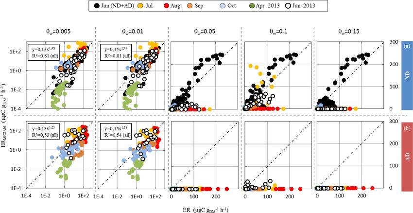
4712                                 A.-C. Genard-Zielinski et al.: Seasonal variations of Q. pubescens isoprene emissions

most severe scenario). The main impact of future drier condi-     sion variations in relation to easily accessible environmental
tions in the Mediterranean was found to be an enhancement         drivers and (ii) process-based relationships built on the un-
(+40 %) of isoprene emissions sensitivity to thermal stress.      derstanding of the ongoing biological regulation (see Ash-
                                                                  worth et al., 2013). Both types of model are adapted for
                                                                  global and regional modelling, but the former are more com-
                                                                  monly used for atmospheric applications, especially for air
1   Introduction                                                  quality exercises for which mechanistic models remain far
                                                                  too complex. Indeed, whilst Grote et al. (2014) have in-
A large number of Mediterranean deciduous and evergreen           dicated that such models are fairly effective in accounting
trees produce and release isoprene (2-methyl-1,3-butadiene,       for the mild stress effects on seasonal isoprene variations of
C5 H8 ). Under non-stress conditions, only 1 %–2 % of the         Quercus ilex, the large number of necessary descriptive pa-
carbon recently assimilated is emitted as isoprene, whereas       rameters continues to represent an obstacle for their broad
under stress conditions such as water scarcity this value         and routine use in air quality (Ashworth et al., 2013). More-
can reach up to 20 %–30 % (Quercus pubescens, Genard-             over, the development of BVOC empirical emission mod-
Zielinski et al., 2014). Although the role of isoprene remains    els, and especially of the most widely used empirical model,
a subject of debate, it seems likely that C5 H8 helps plants      MEGAN (Model of Emissions of Gases and Aerosols from
to optimise CO2 assimilation during temporary and mild            Nature, Guenther et al., 2006, 2012), was partly based on
stresses, especially during the growing and warmer periods        measurements carried out under optimum growing condi-
(Brilli et al., 2007; Loreto and Fineschi, 2015). The major       tions and/or obtained from very few emitters. Therefore, if
role of isoprene in plant defence probably explains its large     they depict a fair picture of the general level and global dis-
annual global emissions (440–660 TgC yr−1 , Guenther et al.,      tribution of BVOC emission, they remain somewhat deficient
2006), forming the largest quantity of all biogenic volatile      in accounting for a large range of stress conditions. When
organic compounds (BVOCs) emitted. Although present in            used for air quality monitoring applications, such a bias in-
the atmosphere at the ppb or ppt level, isoprene has a broad      trinsic to the model can significantly weaken air quality fore-
impact on atmospheric chemistry, both in the gas phase (es-       casts in areas that are greatly influenced by biogenic sources
pecially in the O3 budget of some urbanised areas, Atkinson       (von Kuhlmann et al., 2004; Chaxel and Chollet, 2009). Con-
and Arey, 2003) and in the particulate phase (secondary or-       cerning the impact of drought stress, the inclusion of the soil
ganic aerosols formation, Goldstein and Steiner, 2007), and       moisture effect on isoprene emission in MEGAN was de-
hence on biosphere–atmosphere feedbacks. For instance, in         rived from a sole drought study made on Populus deltoides
the Mediterranean area, Curci et al. (2009) showed that iso-      (Pegoraro et al., 2004). Validation regarding a broader range
prene could be responsible for the production of 4 to 6 ppbv      of environmental conditions (including stress conditions) and
of ozone between June and August, representing 16 %–20 %          emitters is necessary. Weaknesses in accounting for the im-
of total ozone. Given the broad impacts of isoprene on at-        pact of drought can be detrimental to isoprene emission in-
mospheric chemistry, considerable efforts have been made          ventories, especially when undertaken in areas that are cov-
to (i) understand the physiological mechanisms responsible        ered with a large quantity of high isoprene emitters and that
for isoprene synthesis and emission and the different envi-       are subject to frequent drought episodes, like the Mediter-
ronmental parameters that control their variability, in order     ranean region. Moreover, in addition to a predicted temper-
to (ii) develop isoprene emission models that can account for     ature increase of between 1.5 and 3 ◦ C, climate models over
the broadest possible range of environmental conditions.          this area predict an amplification of the natural drought (ND)
   Thus, it has extensively been shown that under non-            during summers due to a reduction in precipitation that could
stressful conditions, isoprene synthesis and emission are         locally reach up to 30 % by the year 2100 (Giorgi and Li-
closely connected and primarily depend upon light and tem-        onello, 2008; Intergovernmental Panel on Climate Change,
perature conditions (Guenther et al., 1991, 1993). In contrast,   2013; Polade et al., 2014). Owing to the close interactions
under environmental stress, isoprene emission and synthe-         between air pollution over large Mediterranean urban ar-
sis are uncoupled in a way that is not fully understood and       eas and strong BVOC emissions from nearby vegetation,
hence still under debate (Affek and Yakir, 2003; Peñuelas and     the potential impacts of future climatic changes on isoprene
Staudt, 2010). Indeed, although some authors have identi-         emissions represent an acute environmental issue needing to
fied an increase in isoprene emission under mild water stress     be addressed (Chameides et al., 1988; Atkinson and Arey,
(Sharkey and Loreto, 1993; Funk et al., 2004; Pegoraro et         1998; Calfapietra et al., 2009; Pacifico et al., 2009). Within
al., 2004; Genard-Zielinski et al., 2014), others have reported   this context, a recent study has underlined the importance
the opposite (Brüggemann and Schnitzler, 2002; Rodriguez-         of monitoring over a long period both isoprene emissions
Calcerrada et al., 2013; Tani et al., 2011).                      and soil moisture in water-limited ecosystems (Zheng et al.,
   Concerning the modelling of isoprene emission variations,      2015). Since Q. pubescens Willd. is the second largest iso-
two main approaches have been considered so far: (i) empir-       prene emitter in Europe (and foremost in the Mediterranean
ically based parameterisations to represent observed emis-        zone) (Keenan et al., 2009), it represents an ideal model

Biogeosciences, 15, 4711–4730, 2018                                                   www.biogeosciences.net/15/4711/2018/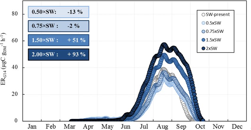
A.-C. Genard-Zielinski et al.: Seasonal variations of Q. pubescens isoprene emissions                                       4713

species by which to investigate isoprene emission variabil-         2.2   Seasonal sampling strategy
ity under drought conditions.
   The objectives of this study were (i) to investigate in          Isoprene emission rate measurements were undertaken for at
natura the influence of natural (ND) and amplified (AD)             least 1 week per month from June 2012 to June 2013, ex-
drought on Q. Pubescens seasonal gas exchanges (CO2 ,               cept for the period from November 2012 until March 2013
H2 O) and in particular isoprene emission rates (ER);               when Q. pubescent is fully senescent, with leaves remaining
(ii) to test and compare two empirical emission models,             on the tree (marcescent species). This calendar enabled us to
MEGAN2.1 (Guenther et al., 2012) and G14 (this study)               capture isoprene emissions during leaf maturity but also dur-
in assessing seasonal ER variability under different drought        ing bud break (April 2013) and just before leaf senescence
intensities; and (iii) to evaluate the sensitivity of ER to fu-     (October 2012). Three trees were studied in each plot along
ture climatic changes (warming and precipitation reduction)         the whole seasonal cycle, with a single branch at the top of
based on two extreme IPCC scenarios: RCP2.6 (moderate)              the canopy predominantly sampled for each tree. More inten-
and RCP8.5 (extreme).                                               sive measurements were carried out in June 2012 (3 weeks)
                                                                    and April 2013 when tree-to-tree and within-canopy variabil-
2     Materials and methods                                         ity was assessed. One ND branch was subsequently sampled
                                                                    throughout all intensive campaigns, and the five other ND
2.1    Experimental site O3 HP                                      and AD branches were alternately sampled during 1 to 2 days
                                                                    (Genard-Zielinski et al., 2015). Isoprene samples were col-
Experimental data were obtained at the O3 HP site (Oak Ob-          lected on cartridges packed with adsorbents, apart from April
servatory at the Observatoire de Haute Provence, 5◦ 420 4400 E,     2013 when online isoprene measurements were conducted
43◦ 550 5400 N). This site constitutes part of the French na-       using a PTR-MS (proton-transfer-reaction mass spectrome-
tional network SOERE F-ORE-T (System of Observation                 ter) directly connected to the enclosure via a 50 m 1/400 PTFE
and Experimentation, in the long term, for Environmen-              line. When cartridges were used, samples (volume ranging
tal Research) dedicated to investigating the functioning of         between 0.45 and 0.9 L, depending on the expected emission
the forest ecosystem. The O3 HP site (680 m above mean              intensity) were taken from sunrise to sunset, roughly every
sea level) is located 60 km north of Marseille and consists         2 h. PTR-MS measurements allowed a higher sampling fre-
of a homogeneous 70–100-year-old coppice dominated by               quency (between 120 and 390 s−1 ).
Q. pubescens (5 m in height; leaf area index, LAI = 2.2),              Branch enclosures were generally installed on the day
which accounts for ≈ 90 % of the biomass and ≈ 75 % of              before the first emission rate measurement was taken and
the trees. A rainout shelter above 300 m2 of the canopy dy-         at least 2 h beforehand in order for the plant to return to
namically excluded rainfall by deploying automated shutters.        normal physiological functioning. Note that although senes-
This facility facilitated the study of Q. pubescens under nat-      cence had just begun in October 2012, we did check that the
ural and amplified drought, henceforth referred to as the ND        enclosed branches were not senescent during these measure-
and AD plot respectively. In the present study, the device          ments.
was deployed during rain events from the end of May un-
til October 2012 in order to exclude 32 % of the precipita-         2.3   Branch-scale isoprene emissions and gas exchanges
tion in the rain exclusion plot. In practice, almost all rainfall
in late spring and summer was thus intercepted, increasing          Sampling was undertaken using two identical dynamic
the number of dry days (< 1 mm, Polade et al., 2014) by 22.         branch enclosures (detailed description in Genard-Zielinski
This percentage corresponds with the highest IPCC projec-           et al., 2015). Briefly, the device consisted of a ≈ 60 L PTFE
tions made for the end of the century over the Mediterranean        (polytetrafluoroethylene) frame closed by a sealed, 50 µm
area and accords with the precipitation reduction at O3 HP          thick PTFE film, to which ambient air was introduced at
during the driest years from 1967 to 2000 compared with the         Q0 ranging between 11 and 14 L min−1 using a PTFE pump
average precipitation over this period. Using an ombrother-         (KNF N 840.1.2 FT.18® , Germany). Gas flow rates were
mic diagram (P < 2T , with P = monthly precipitation in mm          controlled by mass flow controllers (Bronkhorst) and all tub-
and T = monthly air temperature in ◦ C), we assessed that the       ing lines were made of PTFE. A PTFE propeller ensured
summer 2012 drought period reaches 4.5 months in the AD             the rapid mixing of air inside the chamber. The microcli-
plot, compared with 3 months in the ND plot. Ambient and            mate (PAR, photosynthetic active radiation; T ; relative hu-
soil environmental parameters were continuously monitored           midity) inside the chamber was continuously monitored (rel-
using a dense network of sensors (for details see Sect. 2.7).       ative humidity and temperature probe LI-COR 1400–104® ,
Access to the canopy was at two levels: ≈ 0.8 and 3.5 m (top        and quantum sensor LI-COR, PAR-SA 190® ; Lincoln, NE,
canopy branches) above ground level, with the highest level         USA) and recorded (LI-COR 1400® ; Lincoln, NE, USA).
being the one at which we undertook this study. Further de-         CO2 –H2 O exchanges from the enclosed branches were also
scription can be found in Santonja et al. (2015).                   continuously measured using infrared gas analysers (IRGA
                                                                    840A® , LI-COR) in order to assess the net assimilation Pn

www.biogeosciences.net/15/4711/2018/                                                      Biogeosciences, 15, 4711–4730, 2018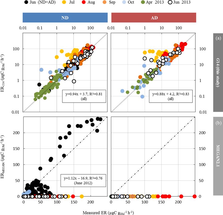
4714                                 A.-C. Genard-Zielinski et al.: Seasonal variations of Q. pubescens isoprene emissions

(in µmolCO2 m−2 s−1 ) and the stomatal conductance to wa-         transmission efficiencies of both instruments were assessed
ter vapour Gw (molH2 O m−2 s−1 ) using the equations from         using a standard gas calibration mixture (TO-14A Aromatic
Von Caemmerer and Farquhar (1981) as detailed in Genard-          Mix, Restek Corporation, Bellefonte, USA; 100 ± 10 ppb in
Zielinski et al. (2015).                                          nitrogen). Assuming an uncertainty of ±15 % in the k-rate
   Total dry biomass matter (DM) was calculated by manu-          constants and in the mass transmission efficiency, the overall
ally scanning every leaf of each sampled branch enclosed in       uncertainty of the concentration measurement is estimated
the chamber and applying a dry leaf mass per area conver-         to be of the order of ±20 %. Background signal was ob-
sion factor (LMA) extrapolated from concomitant measure-          tained by passing air through a platinum catalytic converter
ments made on the same site. The mean (range) DM was 0.16         heated at 300 ◦ C. Detection limits defined as 3 times the stan-
(0.01–0.45) gDM , and mean (range) LMA was 13.17 (0.82–           dard deviation on the background signal were 10 and 50 ppt
36.67) gDM cm−2 .                                                 with the PTR-ToF-MS and the HS-PTR-MS respectively. An
   Isoprene emission rates (ER) were calculated as                intercomparison between both the cartridge + GC-MS and
                                                                  PTR-MS protocols was undertaken parallel to another emit-
ER = Q0 × (Cout − Cin ) × DM−1 ,                           (1)
                                                                  ter present on the site (Acer monspessulanum); no significant
where ER is expressed in µgC g−1        −1
                                   DM h , Q0 is the flow rate     difference was observed between the techniques (Genard-
of the air introduced into the chamber (L h−1 ), Cin and          Zielinski et al., 2015).
Cout are the concentrations in the inflowing and outflowing          The overall uncertainty (sampling + analysis) on ER as-
air (µgC L−1 ), and DM is the sampled dry biomass matter          sessment was between 20 % and 25 %.
(gDM ).
   Throughout the seasonal cycle, except in April, isoprene       2.4   Statistics
was collected using packed cartridges (glass and stainless-
steel) prefilled with Tenax TA and/or Carbotrap. Isoprene         All statistics were performed on STATGRAPHICS® centu-
was then analysed in the laboratory according to a gas            rion XV by Statpoint, Inc. Differences in Pn , Gw , ER, and
chromatography–mass spectrometry (GM-MS) procedure                Q. pubescens isoprene emission factors (εiso,Qp , see Sect. 2.5
detailed in Genard-Zielinski et al. (2015), with a level of an-   for details) between the ND and the AD plot were tested
alytical precision greater than 7.5 %.                            using Mann–Whitney U tests. Seasonal changes in these
   In April 2013, two types of PTR-MS were used for on-           ecophysiological parameters were tested using the Kruskal–
line isoprene sampling and analysis. A quadrupole PTR-            Wallis test and the analysis was performed separately on trees
MS (HS-PTR-MS, Ionicon Analytik GmbH, Innsbruck Aus-              from the ND and AD plot. Comparisons between COOPER-
tria), connected to the ND branch enclosure, was operated         ATE environmental data (see Sect. 2.7) were made using a
at 2.2 mbar pressure, 60 ◦ C temperature, and 500 V voltage       Wilcoxon test when data were not log-normal and a t test
in order to achieve an E/N ratio of ≈ 115 Td (E: elec-            when log-normal.
tric field strength (V cm−1 ); N: buffer gas number density
(molecule cm−3 ); 1 Td = 10−17 V cm2 ). The primary H3 O+         2.5   Branch-scale ER assessment using MEGAN2.1
ion count assessed at m/z 21 was 3×10⁷ cps, with a typically            emission model
< 10 % contribution monitored from the first water cluster
                                                                  Based on the latest version of the MEGAN model
(m/z 37) and < 5 % contribution from the O+   2 (m/z 32). Mea-    (MEGAN2.1, Guenther et al., 2012), Q. pubescens ER were
surements were operated in scan mode (m/z 21 to m/z 210)
                                                                  assessed for the sampling conditions of our seasonal study
every 380 s. After 15–20 min of sampling of incoming air,
                                                                  using
the outgoing air was sampled for 30 to 60 min. A high-
resolution (m/1m ≈ 4000) time-of-flight PTR-MS (PTR-              ERMEGAN = εiso,Qp χQp γiso .                                (2)
ToF-MS-8000, Ionicon Analytik GmbH, Innsbruck Austria)
connected to the second enclosure used in our study enabled         Nota bene: in order to be comparable with our measure-
us to discriminate between compounds when their masses            ments carried out on top canopy leaves and expressed as net
differ at the tenth part. The main experimental characteristics   emission rates in the unit of µgC g−1  −1
                                                                                                     DM h , no canopy envi-
were similar to the HS-PTR-MS, but a voltage of 550 V was         ronment coefficient CCE nor LAI was considered in the cal-
used in order to reach an E/N ratio of ≈ 125 Td. The H3 O+        culation of γiso and thus in ERMEGAN (for further details see
ion count assessed at m/z 21 was 1.1 × 10⁶ cps with a simi-       Guenther et al., 2012).
lar < 10 % contribution monitored from the first water cluster
(m/z 37) and < 2.5 % contribution from the O+     2 (m/z 32).     2.6   Branch-scale ER assessment using an artificial
The signal at m/z 69 corresponding to protonated isoprene               neural network trained on field data
was converted into mixing ratio by using a proton trans-
fer rate constant k of 1.96 × 10⁻⁹ cm3 s−1 (Cappellin et al.,     The artificial neural network (ANN) developed in this study
2012), the reaction time in the drift tube, and the experimen-    to assess branch-scale ER from Q. pubescens (henceforth
tally determined ion transmission efficiency. The relative ion    referred to as G14) was based on a commercial version of

Biogeosciences, 15, 4711–4730, 2018                                                    www.biogeosciences.net/15/4711/2018/
A.-C. Genard-Zielinski et al.: Seasonal variations of Q. pubescens isoprene emissions 4715
the Netral NeuroOne software v.6.0 (http://www.inmodelia. as the PAR reaching all of the top canopy branches stud-
com/, France; last access: 31 July 2018). The ANN was used ied. Ambient air temperature (T , ◦ C) measured at 6.15 m
as a multilayer perceptron (MLP) in order to calculate mul- (CS215, Campbell Scientific Ltd., UK) in the ND and AD
tiple non-linear regressions between a set of input regressors plot was used for both sets of branches. Since some precipi-
xi (the environmental variables measured at the O3 HP) and tation (P , mm) values were missing (< 5 %) from the COOP-
the output data (the measured isoprene ER). The assessed ER ERATE database during our data processing, P values from
(ERG14 ) was calculated as follows: the nearby (< 10 km) Forcalquier meteorological station were
jX
=N
"
i=n
X
!# used. The bias between cumulated P (Pcum ) curves at both
ERG14 = w0 + wj,k × f w0,j + wi,j × xi , (3) sites was assessed and considered in order to extrapolate the
j =1 i=1 missing values at the O3 HP site. As P was cumulated over
where w0 is the connecting weight between the bias and the 7, 14, and 21 days, the resulting bias was negligible (≈ 1 %)
output, N the number of neurons Nj , f the transfer func- and no further adjustment was made. Soil water content (SW,
tion, w0,j the connecting weight between the bias and the L L−1 ) and temperature (ST, ◦ C) at −0.1 m (Hydra Probe II,
neuron Nj , wi the connecting weight between the input and Stevens, Water Monitoring Systems Inc., OR, USA) specific
the neuron Nj , and xi the n input regressors. The MLP op- to each of the sampled trees were selected and extracted from
timisation of the weights w was achieved according to Bois- the COOPERATE database; when soil data were missing,
sard et al. (2008). Every input regressor xi was centrally they were extrapolated from the nearest equivalent data point
normalised. Two sub-datasets were considered, for the ND measurement. Daily mean PAR, T , P , SW, and ST were cu-
and AD plot respectively. For each sub-dataset, 80 % of our mulated over a time period ranging from 1 to 21 days before
data were used for training and optimising the MLP, and the measurement.
the remaining 20 % were used for blind validation based on
root mean square error (RMSE). Training–validation split- 2.8 ORCHIDEE land surface model: providing future
ting was made using a Kullback–Leibler distance function conditions to investigate ER sensitivity to climatic
available in NeuroOne v 6.0. Only the non-linear hyperbolic changes
tangent (tanh) function was tested as transfer function f . Up
to N = 7 neurons (distributed in only one layer) were tested Present-day T and P were assessed as the 2000–2010 daily
for every ANN setting. The overtraining phenomenon (a too- averages derived from the ISI-MIP (Inter-Sectoral Impact
large number of neurons vs. the number of input parameters) Model Intercomparison Project) climate dataset (Warsza-
was checked against the RMSEtraining / RMSEvalidation evolu- wski et al., 2014) over the Mediterranean area. This dataset
tion vs. the number N of neurons tested: training was stopped contains the bias-corrected daily simulation outputs of the
for RMSEtraining > RMSEvalidation when N ≥ 3. Earth system model HadGEM2-ES. Corresponding values
Among the other available statistical methods, ANNs for the 2090–2100 period were used to assess the expected
present the advantage of being the most parsimonious, i.e., range of future climatic changes. They were derived from
giving the smallest error for a same number of descriptors two ISI-MIP future projections forced along two represen-
(see for instance Dreyfus et al., 2002). Moreover, the ANN tative concentration pathways (RCPs): the so-called “peak-
approach, as is the case of other non-linear regression meth- and-decline” greenhouse gas concentration scenario RCP2.6
ods, is not particularly sensitive to regressors’ co-linearity (optimistic or moderate scenario) and the “rising” green-
(Bishop, 1995; Dreyfus et al., 2002). On the other hand, one house gas concentration scenario RCP8.5 (extreme or severe
of the limitations of ANNs is that they can only be employed scenario). All T and P data were extracted for the entire
for interpolation within the range of values of the trained Mediterranean region from the global ISI-MIP dataset and
data, and not for extrapolation exercises beyond this range. subsequently averaged over the area.
Consequently, during the isoprene emission sensitivity to fu- Using these present and future T , P , and PAR values (ISI-
ture climatic changes (see Sect. 2.8), only xi values fitting MIP derived), the corresponding present and future SW and
within the range of variation (±20 %) tested during the train- ST were assessed by running the global land surface model
ing phase were considered; in total 21 % of the data were thus ORCHIDEE (ORganising Carbon and Hydrology In Dy-
rejected. namic EcosystEms) over the European part of the Mediter-
ranean region. The calculated SW and ST were averaged
2.7 COOPERATE environmental database over this area. ORCHIDEE is a spatially explicit, process-
based model that calculates the CO2 , H2 O, and heat fluxes
Ambient and edaphic parameters used for the ANN opti- between the land surface and the atmosphere. Vegetation
misation were obtained from the COOPERATE database species distributed at the Earth’s surface are represented in
(https://cooperate.obs-hp.fr/db, last access: 31 July 2018) ORCHIDEE through 13 plant functional types (PFTs). Pro-
and daily averaged for each day of our study. Ambient PAR cesses in the model are represented at the time step of 0.5 h,
(µmol m−2 s−1 ) measured above the canopy at 6.5 m (LI- but the variations of water and carbon pools are calculated
COR Li-190® ; Lincoln, NE, USA) in the ND plot was used on a daily basis. A detailed description of ORCHIDEE is
www.biogeosciences.net/15/4711/2018/ Biogeosciences, 15, 4711–4730, 20184716 A.-C. Genard-Zielinski et al.: Seasonal variations of Q. pubescens isoprene emissions
provided by Krinner et al. (2005). Simulations over the Euro-
pean part of the Mediterranean region were performed with
the ORCHIDEE model at 0.5 × 0.5◦ spatial resolution us-
ing the soil parameters (clay, silt, and sand fractions) from
Zobler (1986). Given that this study focuses on isoprene
emissions from Q. pubescens, we fixed the vegetation with
the corresponding PFT “temperate broad-leaf summer green
tree”. The described ISI-MIP historical forcings and the ISI-
MIP future projections were used as climate conditions for
ORCHIDEE runs and ER assessment using G14. Equilib-
rium was reached by running ORCHIDEE on the first decade
of the climate forcing (1961–1990) repeated in a loop and the
value of atmospheric CO2 corresponding to the year 1961.
Among the two different hydrology schemes available in
ORCHIDEE, the physically based 11-layer scheme was used
(Guimberteau et al., 2013).
ER sensitivity to moderate and severe temperature and/or
precipitation changes was evaluated using G14 under 6
cases: (i) the T (respectively P ) test was conducted consid-
ering only T and ST (respectively only P and SW) changes
according to the RCP2.6 scenario; (ii) the TT and PP tests
were similar to the T and P tests but considered changes
according to the RCP8.5 scenario; (iii) the T + P (respec-
tively TT + PP) test combined the effect of T , ST, P , and
SW changes according to RCP2.6 (respectively RCP8.5).
3 Results
3.1 Environmental conditions observed at the O3 HP
Mean daily ambient air temperature T varied between −3
and 26 ◦ C (January 2013 and August 2012 respectively,
Fig. 1a). Seasonal PAR variations were in line with T vari-
ations, with the daily mean peaking at 900 µmol m−2 s−1 in
July (Fig. 1b). In 2012, the amplification of the ND was ad-
justed from May to reach its maximum (32 %) in July and
maintained until November when rain exclusion was stopped
(Fig. 1c). The annual Pcum in the AD plot was lower by
273 mm than in the ND plot at the end of 2012 (782 com-
pared to 509 mm). In 2013 the AD started only at the end
of June, simulating a later amplification. From August un-
til October 2012, SW was 50 %–90 % lower in the AD plot
−1
than in the ND plot (≈ 0.02 and to 0.05 LH2 O Lsoil respec-
tively in August, Fig. 1d). The AD plot soil water deficit re- Figure 1. Seasonal variations of daily environmental parameters
mained significant until the end of the experiment (Mann– measured at the O3 HP from March 2012 to June 2013. (a) Ambient
Whitney, P < 0.05 in June 2012, P < 0.001 from July 2012 air temperature T was obtained at 6.5 m above ground level (a.g.l.),
to June 2013), although the rain exclusion system was not approximatively 1.5 m above the canopy. (b) Photosynthetic active
activated between December 2012 and June 2013. radiations PAR received at 6.5 m a.g.l. in the ND plot. (c) Cumu-
No significant difference was noticed for monthly PAR lated precipitation Pcum measured over the ND (blue) and AD (red)
and T means between the ND and the AD plot, except in plot. (d) Mean soil water content SW ± SD measured at −0.1 m
September 2012 when branches sampled on the ND plot re- depth from various soil probes in the ND (blue, n = 3) and AD (red,
n = 5) plot.
ceived significantly more PAR than branches on the AD plot
(Mann–Whitney, P < 0.001). This difference could be due to
an orientation of the branches sampled in the ND plot in
Biogeosciences, 15, 4711–4730, 2018 www.biogeosciences.net/15/4711/2018/A.-C. Genard-Zielinski et al.: Seasonal variations of Q. pubescens isoprene emissions 4717
September that enabled greater receipt of PAR during our
measurements than the AN sampled branches.
3.2 Gas exchange and isoprene seasonal variations
Gw and Pn showed similar seasonal patterns in both plots
(Fig. 2a, b), with the lowest values in July–September
(10–20 molH2 O m−2 s−1 and ≈ 1 µmolCO2 m−2 s−1 respec-
tively) and the highest in June (80–170 molH2 O m 2 s−1 and
≈ 9 µmolCO2 m−2 s−1 respectively). Respiration dominated
over gross CO2 assimilation in April, resulting in negative
net assimilation (Pn ≈ −1 µmolCO2 m−2 s−1 ) in both plots.
In contrast, Gw and Pn were not influenced by water stress in
the same way. Whereas Gw was significantly reduced under
AD from July 2012, Pn remained stable, except in June 2013
when Pn values that were twice as high under AD than ND
were observed. It is important to note that the tomography
measurements made at this site showed that oak roots were
predominantly distributed in the outermost humiferous hori-
zon located above a calcareous slab at a 10–20 cm depth and
that only very few roots crossed this slab.
Water stress only affected the ER seasonal pattern during
summer (Fig. 2c). Maximum ER was delayed by a month in
the AD plot (104.8 µgC g−1 DM h
−1 in August) in comparison
−1 −1
to the ND plot (78.5 µgC gDM h in July). ER was lowest in
October (≈ 6 µgC g−1 DM h
−1 in both plots). During April bud
break and isoprene emission onset, ER was as low as 0.5 and
1 µgC g−1DM h
−1 in the ND and AD plot respectively.
Although εiso,Qp was calculated every month as the slope
of ER vs. CL × CT (as in Guenther et al., 1995), this cor-
relation was not significant in July, especially in the case
of AD branches (P > 0.05, R 2 = 0.06 and 0.01 for ND and
AD respectively). As a result, εiso,Qp in July was calculated
by averaging ER measured under environmental conditions
close to 1000 ± 100 µmol m−2 s−1 and 30 ± 1 ◦ C. In gen-
eral, AD branches showed poorer ER vs. CL × CT correla-
tions than branches growing in the ND plot (data not shown).
εiso,Qp was significantly higher by a factor of 2 in August
and September for the AD branches compared to the ND
(Fig. 2d). As for ER, εiso,Qp maximum was reached in August
(137.8 µgC g−1 −1
DM h ) in the AD plot, while the maximum in Figure 2. Seasonal variations of monthly Q. pubescens gas ex-
the ND plot occurred in July (74.3 µgC g−1 −1
DM h ). The gen- changes observed at O3 HP (June 2012 to June 2013) under ND
eral high variability observed in April during the isoprene (blue) and AD (red) (mean ± SD). (a) Stomatal conductance to wa-
emission onset (some branches were already emitting, while ter vapour Gw . (b) Net photosynthetic assimilation Pn . (c) Mea-
some were not yet emitting isoprene, regardless of their lo- sured branch isoprene emission rate ER. (d) Isoprene emission fac-
cations in the AD / ND plots) was as large as the AD–ND tor (Is ) calculated according to Guenther et al. (1995) using in situ
variability and thus could not solely be attributed to the wa- ER vs. CL × CT correlations, except in July where mean ER mea-
ter stress treatment. The relative annual εiso,Qp difference be- sured under enclosure conditions close to 1000 µmol m−2 s−1 and
30 ◦ C was used. Differences between ND and AD using Mann–
tween ND and AD was +45 %.
Whitney U tests are denoted using lower case letters (a > b > c > d).
Differences among water treatment stress using Kruskal–Wallis
3.3 Modelling the isoprene seasonal variations of
tests are denoted by asterisks (*: P < 0.05; **: P < 0.01; ***:
Q. pubescens at the O3 HP P < 0.001).
Given that we were aiming to test the capacity of an em-
pirically based isoprene emission model to describe seasonal
www.biogeosciences.net/15/4711/2018/ Biogeosciences, 15, 4711–4730, 20184718 A.-C. Genard-Zielinski et al.: Seasonal variations of Q. pubescens isoprene emissions
Figure 3. Comparison between isoprene emission rates (in µgC g−1 −1
DM h ) calculated using MEGAN2.1 (ERMEGAN , Guenther et al., 2012)
and measured isoprene emission rates (ER) vs. the wilting point value θw (0.005 to 0.15 m3 m−3 ), from June 2012 to June 2013, under (a)
ND (n = 267) and (b) AD (n = 138). Since the rain exclusion device was only implemented soon prior to our study’s commencement in June
2012, the ND and AD measurements were considered together for June 2012. Linear regressions for ND June 2012 were y = 1.13x − 12.05,
R 2 = 0.80 (θ w = 0.05 m3 m−3 ); y = 1.13x −7.13, R 2 = 0.80 (θw = 0.1 m3 m−3 ); and y = 1.12x −16.94, R 2 = 0.76 (θw = 0.15 m3 m−3 ).
The dotted line is the 1 : 1 line.
ER variability and sensitivity to drought observed during this sessment for both treatments. On the contrary, for θw ≥
study, we tested the latest version of the MEGAN model, 0.05 m3 m−3 , most of the isoprene emissions were set to zero
which is widely used for air quality and climate change ap- by MEGAN2.1 in the AD plot, while in the ND only June
plications (MEGAN2.1, Guenther et al., 2012). In particu- observations were correctly assessed with an overall over-
lar, the ability of its soil moisture coefficient activity γSM estimation (regardless of the θw values) of ≈ 10 % (R 2 rang-
(Eq. 4a–c) to assess the observed effect of ND and AD ing from 0.76 to 0.80 for θw = 0.15 and 0.1 m3 m−3 respec-
treatments was examined over wilting point θw values rang- tively). If some of the July ERMEGAN were fairly close to
ing from 0.01 to 0.15 m3 m−3 , which is representative of a the observations for θw = 0.1 m3 m−3 , the overall correlation
large brand of soils (Ghanbarian-Alavijeh and Millàn, 2009). was poor (y = 0.2x + 49.5, R 2 = 002).
Indeed, Müller et al. (2008) showed that isoprene assess- Assuming that the discrepancies between ERMEGAN and
ments were very sensitive to θw . For the record, θw was ER only resulted from the γSM formulation in MEGAN2.1
0.15 m3 m−3 at the O3 HP. (and not from the other activity coefficients γP , γT , or γA
Assessed (ERMEGAN ) and observed (ER) isoprene emis- used, Eq. 3), ER / ERMEGAN was calculated for both ND
sion rates were compared separately for ND and AD. How- and AD treatments and was considered against the measured
ever, given that the rainout shelter was implemented close to SW. In the ND treatment, ER / ERMEGAN was not found to
the commencement of our study in June 2012, measurements be significantly dependent on SW (y = 0.653e10.52x , R 2 =
carried out in the AD plot were not distinguished, only in the 0.13, Fig. 4a). However, in the AD plot, ER / ERMEGAN
case of this month, from the ones taken in the ND plot (AD increased exponentially with SW (y = 0.192e51.93x , R 2 =
and ND data were thus mixed for June 2012). 0.66, Fig. 4b) and in particular when SW became higher
For θw < 0.05 m3 m−3 , and regardless of the θw value, than the wilting point θw measured at the O3 HP site
MEGAN2.1 captured more than 80 % of the ER variability (0.15 m3 m−3 ). Similar findings were obtained for SW-7,
in the ND plot (y = 0.15x 1,5 , R 2 = 0.81, Fig. 3a), but less SW-14 and SW-21, for both the ND and AD treatments (Ta-
(≈ 50 %) in the AD plot (R 2 = 0.53 and 0.54 for θw = 0.005 ble 1).
and 0.01 m3 m−3 respectively, Fig. 3b). An overall over- In order to provide a better description of the impacts of
estimation of 25 % was associated with the MEGAN2.1 as- ND and AD on ER as observed at the O3 HP, an empirical
Biogeosciences, 15, 4711–4730, 2018 www.biogeosciences.net/15/4711/2018/A.-C. Genard-Zielinski et al.: Seasonal variations of Q. pubescens isoprene emissions 4719
Figure 4. Ratio between observed (ER) and calculated (ERMEGAN ) isoprene emission rates vs. the soil water content SW measured at the
O3 HP, under (a) ND (n = 267) and (b) AD (n = 138). Given that the rain exclusion device was only implemented just before our study began
in June 2012, the ND and AD measurements were considered together for June 2012. The dotted line is for SW = θw measured at O3 HP
(0.15 m3 m−3 ).
type model, based on ANN optimisation of our observations ment (ND or AD) and the month, except in July (Fig. 5a),
at the O3 HP, was developed specifically for Q. pubescens when ER variability was always poorly represented regard-
isoprene emissions. Training and validation of the differ- less of the different ANN settings considered. July corre-
ent ANNs tested were made using values of ER, T , P , sponds to the period where trees started to adapt to ND and
PAR, ST, and SW measured at the O3 HP (COOPERATE AD; this period was possibly insufficiently represented in
database). Environmental regressors xi were integrated, us- our dataset to be well taken into account by our statistical
ing daily means, over a period ranging from 0 to 21 days approach. An overall underestimation of 6 % and 12 % was
prior to the measurements. observed in the ND and AD respectively. For comparison,
Among the different ANN settings tested, an optimised ar- ERMEGAN calculated with a value θw of 0.15 m3 m−3 are pre-
chitecture, G14 (lowest RMSE between calculated and mea- sented again in Fig. 5b for both the ND and AD treatment.
sured values, no overtraining, best correlation between mea- Under ND, the global contribution of the two lowest fre-
sured and calculated ER over the whole range of value, quencies (−14 and −21 days) considered in G14 was, rel-
see Boissard et al., 2008), was found for N = 3 and a ative to the contribution of the two highest frequencies (in-
set of 16 xi with their corresponding connecting weights stantaneous and −7 days), higher than under AD (Fig. 6). In
wi (Appendix A). The final optimised RMSE (validation particular, in October 2012 and April and June 2013, the two
data) was 8.5 µgC g−1 −1
DM h , for ER values ranging from lowest frequencies respectively represented 20 %, 97 %, and
−1 −1 50 % of the total in the ND compared to 3 %, 55 %, and 26 %
0.06 to 113 µgC gDM h , and represents 35 % of the mean
(22.7 µgC g−1 −1 in the AD.
DM h ). More than 80 % of the ER seasonal vari-
ations were assessed by G14, regardless of the water treat-
www.biogeosciences.net/15/4711/2018/ Biogeosciences, 15, 4711–4730, 20184720 A.-C. Genard-Zielinski et al.: Seasonal variations of Q. pubescens isoprene emissions
Table 1. Correlations between ERMEGAN / ER and the soil water content (SW) cumulated over 7 to 21 days before the measurement.
ERMEGAN and ER are isoprene emission rates calculated using MEGAN2.1 (Guenther et al., 2012) and measured (this study) respectively.
ND AD
x ER / ERMEGAN = f (x) R 2 value ER / ERMEGAN = f (x) R 2 value
SW 0.653e10.5x 0.13 0.192e51.1x 0.66
SW-7 0.715e1.30x 0.13 0.239e6.30x 0.55
SW-14 0.763e0.57x 0.11 0.279e2.74x 0.48
SW-21 0.523e0.46x 0.14 0.365e1.47x 0.38
Figure 5. Calculated vs. measured isoprene emission rates (in µgC g−1 −1
DM h ) under ND (n = 267) and AD (n = 138) from June 2012 to
June 2013, using the (a) G14 (this study) and (b) MEGAN2.1 isoprene model (Guenther et al., 2012) with a wilting point value θ w of
0.15 m3 m−3 (measured at the O3 HP). The dotted line is the 1 : 1 line.
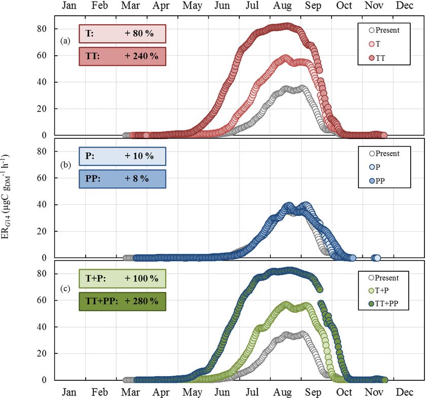
3.4 ER sensitivity to expected climatic changes over the PAR relative changes were not considered as they were neg-
European Mediterranean area ligible for both moderate and severe scenarios.
Moderate changes of the environmental conditions
(RCP2.6 scenario) implied a systematic positive monthly 1T
Present and future T , P , and PAR (ISI-MIP derived) as well throughout the year, whereas 1P was found to be posi-
as SW and ST (ORCHIDEE derived) were integrated over tive only during the winter and negative during the summer
periods ranging from 0 to 21 days in order to be used in G14 (Fig. 7a). ST and SW changes were found to be in line with
and to assess ERG14 for present and future cases. Moderate T and P respectively. The highest monthly relative changes
(respectively severe) changes with regard to the present of were for P (+75 % in February and −30 % in July), whereas
SW, P , ST, T , and PAR were additionally calculated accord- the smallest were for SW. Monthly ST and T relative changes
ing to the RCP2.6 (respectively RCP8.5) scenario; however,
Biogeosciences, 15, 4711–4730, 2018 www.biogeosciences.net/15/4711/2018/A.-C. Genard-Zielinski et al.: Seasonal variations of Q. pubescens isoprene emissions 4721
Figure 6. Seasonal variations of the relative contribution of the different frequencies as considered in G14 (0, 7, 14, and 21 days before the
measurement) among the regressor xi selected in G14, under (a) ND (n = 267) and (b) AD (n = 138). The frequency “0”, “−7”, “−14”,
“−21” includes the contribution of “L-1, T -1, SW-1, T 0, L0, TM -Tm ”; “SW-7, ST-7, P -7”; “T -14, SW-14, ST-14, P -14”; and “T -21,
SW-21, P -21” respectively.
Table 2. Annual absolute and relative changes to the present of SW, P , ST and T according to the RCP2.6 and RCP8.5 scenarios. Present
and future cases were calculated for 2000–2010 and 2090–2100 respectively.
1SW 1Pcum 1ST 1T 1SW / SW 1Pcum /Pcum 1ST / ST 1T /T
(m3 m−3 ) (mm) (◦ C) (%)
RCP2.6 +0.004 +30 +1.4 +1.4 +0.5 +5 +8.4 +9.1
RCP8.5 −0.007 +30 +5.3 +5.3 −5.0 −24 +32 +34
remained more or less constant (between +7 % and +10 %) pacts of changes in temperature and precipitation were con-
between February and November. Overall, T and Pcum ab- sidered, ERG14 was found to systemically increase all year
solute (relative) annual changes were +1.4 ◦ C and +34 mm round, following a seasonal trend that was extremely close
respectively (+9.1 % and +4.8 % respectively, Table 2). to that found for the T and TT tests (Fig. 8c). However, the
Under more severe environmental changes (RCP8.5 sce- additional effect of the precipitation changes enhanced the
nario), monthly T and ST increased all year round, whereas increase noticed for temperature changes only: the annual
P and SW generally decreased, except in January, Febru- increase was +100 % (T + P ) and +280 % (TT + PP) com-
ary, and November, when relative P changes were negligi- pared to +80 % (T ) and +240 % (TT). Note that the ERG14
ble (Fig. 7b). The annual absolute (relative) changes for T seasonal trend calculated for the present did not match our
and Pcum were +5.3 ◦ C and −124 mm respectively (+34 % observed ER variations. Indeed ERG14 was tuned using envi-
and −24 % respectively, Table 2). In these conditions, the an- ronmental parameters averaged over 24 h (and therefore in-
nual 1Pcum /Pcum was similar to the reduction experienced at tegrated over the daytime and nighttime period), which were
the O3 HP during our study (−30 %). The highest monthly thus much lower than the environmental parameters mea-
relative changes were found for ST: +96 % and +86 % sured during our daytime-only samplings (especially for PAR
in January and December respectively. During summertime and T ).
the highest relative changes were found for P (−55 % and
−62 % in July and August respectively). 4 Discussion
ERG14 was found to systematically increase compared to
the present under T and TT changes, with an annual rela- 4.1 Impact of water stress on seasonal gas exchanges
tive change of +80 % and +240 % respectively (Fig. 8a). The and isoprene emission of Q. pubescens
highest relative changes were noted in June and July. In con-
trast, ERG14 was almost not sensitive to P or PP changes, In spite of a significant Gw reduction in summer 2012 owing
regardless of the month (annual relative change of +10 % to the AD, Q. pubescens maintained a positive Pn during the
and +8 % respectively, Fig. 8b). When the combined im- summer, regardless of water stress (ND or AD). Electric re-
sistivity tomography measurements carried out on the O3 HP
www.biogeosciences.net/15/4711/2018/ Biogeosciences, 15, 4711–4730, 20184722 A.-C. Genard-Zielinski et al.: Seasonal variations of Q. pubescens isoprene emissions
applied during 2012, the observed difference was probably
due to the high natural variability in bud breaking and iso-
prene emission onset at this point of the year. The observed
significant increase (a factor of 2) in εiso,Qp under AD (Au-
gust and September) illustrates how isoprene is likely to be
important for short-term Q. pubescens drought resistance,
in particular through the ability of isoprene to stabilise the
thylakoids membrane, under (for example) thermal or ox-
idative stress (Peñuelas et al., 2005; Velikova et al., 2012).
Moreover, previous studies have highlighted the possibility
for a plant growing under water stress to synthesise isoprene
using an alternative carbon source (extra-chloroplastic car-
bohydrates) (Lichtenthaler et al., 1997; Funk et al., 2004;
Brilli et al., 2007). For species emitting other BVOCs than
isoprene, but studied in the Mediterranean area under wa-
ter stress, Lavoir et al. (2009) reported lower (a factor of
≈ 2) monoterpene emission rates from Quercus ilex under
AD from June to August, during the second and third year
of rain exclusion. Since Q. ilex does not possess specific
leaf reservoirs for monoterpene storage, Q. ilex monoterpene
emissions are hence de novo and their emissions are tightly
related to their synthesis according to light and temperature
Figure 7. Seasonal variations between present (2000–2010) and fu- as isoprene.
ture (2090–2100) relative changes of SW, P , ST, and T over the The significant uncoupling between ER and CL × CT re-
continental Mediterranean area obtained using (a) RCP2.6 and (b) ported for the July measurements occurred when SW sig-
RCP8.5 projections. nificantly decreased to their seasonal minimum values (0.05
and 0.03 m3 m−3 ) at the O3 HP in both plots. A similar un-
coupling has also been observed for some other strong iso-
site revealed the heterogeneity of the karstic substrate, organ- prene emitters under water stress (Quercus serrata and Quer-
ised as soil pockets developed between limestone rocks. Wa- cus crispula, Tani et al., 2011). These findings may confirm
ter and nutrient pools and dynamics probably differed greatly these authors’ assumptions that extra-chloroplastic isoprene
between the shallow upper soil layers and the soil pockets de- precursors supply the carbon basis for isoprene biosynthesis
veloped between limestone rocks. However, the soil trenches (and not only from CO2 fixed instantaneously in the chloro-
in the site revealed that a calcareous slab often developed at plast) when water stress occurs, which explains why isoprene
a depth of 10–20 cm and that the roots of the oaks were often emissions become less dependent on the classical abiotic fac-
distributed in this humiferous horizon close to the surface, tors PAR and T as considered by Guenther et al. (1995).
with very few roots crossing this slab. Water supply from
layers deeper than 10–20 cm was thus not considered. Such 4.2 Improving consideration of the drought effect in
behaviour enables trees to limit evapotranspiration under wa- isoprene emission models
ter stress, as a drought-acclimated species permits them to
ensure sufficient accumulation of carbohydrates for the win- Since ND and AD conditions tested by Q. pubescens in
ter (Chaves et al., 2002). Such a strategy was also observed our study stood aside from optimal growth conditions un-
in a study conducted on the same species but under green- der which empirical emission models perform fairly well, it
house conditions (Genard-Zielinski et al., 2015). The sea- was interesting to test the ability of MEGAN2.1 to repro-
sonal regulation and conservation of Pn and Gw enabled iso- duce the observed impacts of a water deficit, as in O3 HP,
prene emissions to be maintained even during the summer on isoprene emissions. The formulation of the MEGAN2.1
water stress (ND and AD). soil moisture factor γSM , wilting point centred, was deemed
The maximum εiso,Qp in both plots was close to previ- inadequate for reproducing the observed isoprene variabil-
ously measured values obtained for the same species un- ity of a drought-adapted emitter such as Q. pubescens. Thus,
der Mediterranean conditions during greenhouse and in situ MEGAN2.1 very successfully reproduced observed ER vari-
experiments (114.3 and 134.7 µgC g−1 −1
DM h ) by Genard- ability under the ND (more than 80 %) only when γSM was
Zielinski et al. (2015) and Simon et al. (2005) respectively. not operating; in fact, only when very low values of the wilt-
The difference observed in April 2013 between εiso,Qp in the ing point were selected (θw ≤ 0.01 m3 m−3 ), γSM was set to
ND and AD could not be attributed solely to the AD effect. 1. In practice, wilting point values lower than 0.01 m3 m−3
Indeed, apart from a possible “memory effect” of the AD are encountered very rarely, and only for loamy sand soils
Biogeosciences, 15, 4711–4730, 2018 www.biogeosciences.net/15/4711/2018/A.-C. Genard-Zielinski et al.: Seasonal variations of Q. pubescens isoprene emissions 4723
Figure 8. Sensitivity of the seasonal variation of isoprene emission rates calculated using G14 (ERG14 , in µgC g−1 −1
DM h , this study) to (a) T
and ST changes as in RCP2.6 (T case) and RCP8.5 (TT case) respectively; (b) SW and P changes as in RCP2.6 (P case) and RCP8.5 (PP
case) respectively; and (c) combined T , ST, P , and SW changes as in RCP2.6 (T + P case) and RCP8.5 (TT + PP case) respectively. Present
and future cases were calculated for 2000–2010 and 2090–2100 respectively. Overall annual relative changes to present are framed.
(Ghanbarian-Alavijeh and Millàn, 2009), and so did not ap- (i.e., the AD treatment, Fig. 4b). Thus, for a species that is
ply in the case of Q. pubescens in the present study. Once not adapted to drought, such as Populus deltoides, the ap-
higher θw values (≥ 0.05 m3 m−3 ) were tested, γSM , and with pearance of unusual water stress conditions would strongly
it almost all the isoprene emissions, rapidly decreased to zero affect and limit its isoprene emissions, as previously reported
once the drought was underway (i.e., after the June measure- by Pegoraro et al. (2004). Indeed, this reference is the only
ments). On a larger scale (over subtropical Africa), Müller one used by Guenther et al. (2006) to account for the im-
et al. (2008) found that MEGAN underestimation of iso- pact of the soil water content in MEGAN2.1; the γSM fac-
prene emissions was also the largest after the drought was tor cannot effectively account for isoprene emission vari-
reached. Consequently, for a drought-adapted isoprene emit- ability for drought-adapted emitters such as Q. pubescens.
ter, not only was the wilting point not found to be a relevant Such a discrepancy under conditions other than Mediter-
parameter to be considered in the expression of γSM , but also ranean was also noticed by Potosnak et al. (2014) during
a formulation that could stop isoprene emissions, regardless a seasonal study over a mixed broad-leaf forest primarily
of the drought intensity. composed of Q. alba L. and Q. velutina Lam. (Missouri,
The fact that under ND the discrepancies between USA). Guenther et al. (2013) have suggested that including
ERMEGAN and ER were not found to be contingent on the the soil moisture averaged over longer periods of time (such
soil water content SW (Fig. 4a) illustrates that under a natural as the previous month and not only the mean over the previ-
drought intensity the capacity of a drought-resistant species ous 240 h) may help to improve predictions during drought
to emit isoprene, that is to trigger physiological regulations periods. In this study we found that the discrepancies be-
to protect its cellular structures, is primarily due to its natural tween ERMEGAN and ER were not related to the frequency
adaptation, and not to the water available in the soil. Isoprene over which SW was considered (Table 1): under ND they
emissions became SW dependent only when the adaptation remained SW independent, whereas under AD the correla-
of Q. pubescens to its “natural” environment was threatened tion between ER / ERMEGAN and SW remained of the same
www.biogeosciences.net/15/4711/2018/ Biogeosciences, 15, 4711–4730, 20184724 A.-C. Genard-Zielinski et al.: Seasonal variations of Q. pubescens isoprene emissions
order (0.66 ≤ R 2 ≤ 0.38) but with a best fit found for the
soil water content of the current day. These findings sug-
gest that the formulation of the soil moisture activity fac-
tor could be improved in MEGAN2.1 if at least two dis-
tinct types of isoprene emitters were considered: (i) non-
drought-adapted species (such as Populus deltoides) from
which isoprene emissions would be modulated using the ac-
tual γSM formulation and (ii) drought-adapted emitters (such
as Q. pubescens), for which γSM would modulate isoprene
emissions relative to SW, without diminishing them to zero,
in an exponential way similar to the expression found in this
study, γSM = 0.192e51.93 SW (see Sect. 3.3). However, valida- Figure 9. Sensitivity of the seasonal variation of isoprene emission
tion of such an expression to other drought-adapted isoprene rates calculated using G14 (ERG14 , in µgC g−1 −1
DM h ) to SW. Over-
emitters, as well as to other drought-adapted BVOC emitters, all annual relative changes to present (2000–2010) are framed.
is required and will necessitate further field and controlled ad
hoc experiments.
Moreover, the largest discrepancies between ERMEGAN 4.3 How will climatic changes affect the seasonal
and ER were noticed for the measurements in April and for variations of Q. pubescens isoprene emissions in the
some of those in June (Figs. 3 and 4), i.e., in periods when Mediterranean area?
the drought (whether natural or amplified) was yet to be com-
pletely underway during our study. This highlights that ER In the future, the Mediterranean area investigated in this
variability during the onset and seasonal increase in isoprene study will face changes in terms of precipitation regime (thus
emissions was not solely drought or SW dependent, even of soil water content) and/or changes in ambient tempera-
in a water-limited environment such as the O3 HP. Indeed, ture (thus of soil temperature). Depending on the CO2 tra-
as observed for Q. alba and Q. macrocarpa Michx, the iso- jectory scenario considered, the annual Pcum would remain
prene onset was found to be strongly correlated with ambient more or less stable (RCP2.6), or decrease by 24 % (RCP8.5);
temperature cumulated over ≈ 2 weeks (200 to 300 degree however, the seasonal regime would change, with a sum-
day, Dd, ◦ C), while the maximum ER was observed at 600– mer reduction of P in both cases. The O3 HP experimental
700 Dd ◦ C (respectively Geron et al., 2000 and Petron et al., strategy used in this work illustrates the upper limit of the
2001). However, if part of this dynamical regulation is al- drought intensity that Q. pubescens could undergo by 2100
ready included in MEGAN2.1 through its emission activity in the Mediterranean area. On the other hand, temperature
factors γT and γA (see Eq. 3), the combined effect of tem- would increase regardless of the scenario and month, from
perature regulation and drought is not fully accounted for. 1.4 (+10 %) to 5.3 ◦ C (+34 %) annually.
For instance, Wiberley et al. (2005) observed that the onset As expected, ERG14 was found to increase appreciably
of kudzu isoprene emissions was shortened by 1 week un- with temperature increase, from 80 % annually in the RCP2.6
der elevated temperature compared to cold growth. ERG14 scenario to 240 % in RCP8.5 (Fig. 8a). If such an increase is
consequently became more sensitive to rapid environmental generally estimated and observed when considering a range
changes as drought intensity increased: the overall averaged of temperature enhancements that accord with future pro-
relative contributions of the regressors xi cumulated over 14 jected changes (Peñuelas and Staudt, 2010), such a response
and 21 days decreased by 45 % and 29 % in the ND and AD seems fairly unclear under Mediterranean water deficit con-
respectively. Interestingly, these changes were found to be ditions (Llusià et al., 2008, 2009). On a global scale, Müller
highest during the months of October 2012 (35 % and 8 % et al. (2008) estimated a 20 % decrease in isoprene due to
in the ND and AD respectively), April 2013 (from 96 % to soil water stress. In our case, isoprene emissions were found
55 % in the ND and AD respectively), and June 2013 (49 % to be scarcely sensitive to P , regardless of the intensity of
and 26 % in the ND and AD respectively, Fig. 6). There- changes: at most, annual P would increase isoprene emis-
fore, during the senescence and onset periods, the drought sions by 10 %, regardless of the intensity of P changes in-
affected the dynamical regulation of isoprene emission more vestigated over the scenario considered (Fig. 8b). This find-
than the emissions themselves. Thus, an ANN approach as ing is in line with our observations: except in October 2012,
used in this study to develop G14 highlights the importance monthly averaged ER were not significantly different in the
of including a modulation along the season of the range of ND and the AD (Fig. 2c). However, if the observed SW did
frequencies over which the relevant environment regressors differ between the ND and the AD plots (≈ a factor of 2,
should be considered. Fig. 1), SW calculated by the ORCHIDEE model was al-
most entirely unaffected by the P changes, even in the se-
vere scenario RCP8.5. Such an uncoupling between P and
SW could be explained by modifications in the ORCHIDEE
Biogeosciences, 15, 4711–4730, 2018 www.biogeosciences.net/15/4711/2018/You can also read