On the contribution of grain boundary sliding type creep to firn densification - an assessment using an optimization approach
←
→
Page content transcription
If your browser does not render page correctly, please read the page content below
The Cryosphere, 16, 143–158, 2022
https://doi.org/10.5194/tc-16-143-2022
© Author(s) 2022. This work is distributed under
the Creative Commons Attribution 4.0 License.

On the contribution of grain boundary sliding type creep to firn
densification – an assessment using an optimization approach
Timm Schultz1 , Ralf Müller1 , Dietmar Gross2 , and Angelika Humbert3,4
1 Instituteof Applied Mechanics, Technische Universität Kaiserslautern, Kaiserslautern, Germany
2 Division of Solid Mechanics, Technische Universität Darmstadt, Darmstadt, Germany
3 Alfred-Wegener-Institut Helmholtz-Zentrum für Polar- und Meeresforschung, Bremerhaven, Germany
4 Faculty of Geosciences, University of Bremen, Bremen, Germany

Correspondence: Timm Schultz (tschultz@rhrk.uni-kl.de)

Received: 26 February 2021 – Discussion started: 12 March 2021
Revised: 17 November 2021 – Accepted: 4 December 2021 – Published: 14 January 2022

Abstract. Simulation approaches to firn densification often        1   Introduction
rely on the assumption that grain boundary sliding is the
leading process driving the first stage of densification. Al-
ley (1987) first developed a process-based material model          Firn densification models fall into two basic categories. Mod-
of firn that describes this process. However, often so-called      els in the first category, which includes most existing mod-
semi-empirical models are favored over the physical descrip-       els, follow the so-called semi-empirical approach of Herron
tion of grain boundary sliding owing to their simplicity and       and Langway (1980), which itself is based on Sorge’s law
the uncertainties regarding model parameters. In this study,       (Bader, 1954) and the Robin hypothesis (Robin, 1958). Ex-
we assessed the applicability of the grain boundary sliding        amples are the models of Arthern et al. (2010), Ligtenberg
model of Alley (1987) to firn using a numeric firn densifica-      et al. (2011), and Simonsen et al. (2013). The empirical pa-
tion model and an optimization approach, for which we for-         rameters of these models are typically adjusted on the basis
mulated variants of the constitutive relation of Alley (1987).     of certain datasets of depth density profiles. In the second
An efficient model implementation based on an updated La-          category of firn densification models, an attempt is made to
grangian numerical scheme enabled us to perform a large            quantify the physical processes related to firn densification.
number of simulations to test different model parameters and       These processes include various types of creep and diffu-
identify the simulation results that best reproduced 159 firn      sion. Micromechanical models are used for small-scale in-
density profiles from Greenland and Antarctica. For most of        vestigations (Johnson and Hopkins, 2005; Theile et al., 2011;
the investigated locations, the simulated and measured firn        Fourtenau et al., 2020), whereas models based on continuum
density profiles were in good agreement. This result implies       mechanics can be used for large-scale simulations. Examples
that the constitutive relation of Alley (1987) characterizes the   of the latter are the models of Arthern and Wingham (1998),
first stage of firn densification well when suitable model pa-     Arnaud et al. (2000), and Goujon et al. (2003).
rameters are used. An analysis of the parameters that result in       Alley (1987) first applied the theory of grain boundary
the best agreement revealed a dependence on the mean sur-          sliding adopted from Raj and Ashby (1971) to firn den-
face mass balance. This finding may indicate that the load         sification at densities below the critical density of ρc =
is insufficiently described, as the lateral components of the      550 kg m−3 . The description of this process by Alley (1987)
stress tensor are usually neglected in one-dimensional mod-        was subsequently used in other firn densification models
els of the firn column.                                            (Arthern and Wingham, 1998; Arnaud et al., 2000; Goujon
                                                                   et al., 2003; Bréant et al., 2017). However, the assumption
                                                                   that grain boundary sliding is the dominant process in firn
                                                                   densification at densities below ρc = 550 kg m−3 has been
                                                                   questioned numerous times (Ignat and Frost, 1987; Roscoat

Published by Copernicus Publications on behalf of the European Geosciences Union.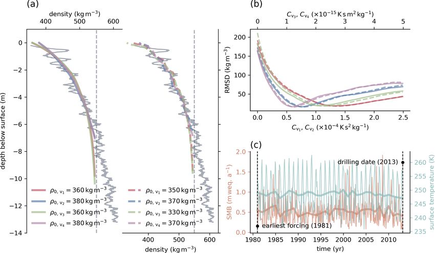
144                                    T. Schultz et al.: Assessment of a grain boundary sliding model for firn densification

et al., 2010). For example, Theile et al. (2011) conducted ex-      sity and forcing data used are described. A detailed descrip-
periments on a small number of snow samples and suggested           tion of the model is presented in the Appendix (Sect. A).
that densification is more likely driven by processes within
the grain rather than by the intergranular process of grain         2.1   Constitutive relation for grain boundary sliding
boundary sliding.
   In this study, we aim to evaluate (i) whether the descrip-       We explain briefly the components and characteristics of the
tion of grain boundary sliding given by Alley (1987) is suit-       constitutive law of Alley (1987) describing the process of
able for the simulation of firn densification at low density,       grain boundary sliding.
(ii) how a modification of the constitutive relation introduced
                                                                           2 8DBD  1 ρice 3

by Bréant et al. (2017) affects simulation results, (iii) whether                                 5 ρ
                                                                    ε̇zz = −δb                1 −          σzz ,
hidden or additional dependencies on climatic or other con-               15 kb T h2 rµ2 ρ        3 ρice
ditions can be identified in the constitutive relation, and

                                                                                    QBD
(iv) how the constitutive relation of Alley (1987) might be         DBD = ABD exp −                                                (1)
                                                                                    RT
improved. Note that our study aims to assess the constitu-
tive relation for grain boundary sliding proposed by Alley          The factor of 2/15 results from the geometric deviation
(1987). An evaluation that clarifies whether grain bound-           pointed out by Alley (1987). Another geometric parame-
ary sliding is the dominant process driving firn densification      ter, δb , describes the width of the grain boundary.
below the critical density of ρc = 550 kg m−3 must be con-             The following part of the equation describes the recip-
ducted using other methods. Experimental attempts to do so          rocal bond or boundary viscosity (Raj and Ashby, 1971).
have been made by, for example, Kinosita (1967), Ignat and          The optimization approach of Alley (1987) was intended to
Frost (1987), and Theile et al. (2011). In contrast to these        identify the optimal values of the boundary viscosity. Alley
experimental investigations, a data-driven model approach is        (1987) compared the results of this optimization to the de-
used in our study. Since the original study of Alley (1987)         scription of the boundary viscosity given by Raj and Ashby
was published, the number of available data have increased          (1971), which includes the volume of the H2 O molecule ,
greatly. The data include a large number of firn profiles and       the Boltzmann constant kb , the temperature T , and the ampli-
forcing data, and they allow us to simulate firn profiles at        tude of grain boundary obstructions h. The latter is a measure
very high quality using additional modeling techniques.             of the roughness of the grain boundary. DBD is an Arrhenius
                                                                    factor describing the rate of boundary diffusion. Values of
                                                                    the typical activation energy for this process, QBD , and the
                                                                    corresponding prefactor, ABD , can be found in the literature
2     Methods                                                       (e.g., Maeno and Ebinuma, 1983) and are further discussed
                                                                    in Sect. 2.2. R is the universal gas constant.
To test the description of grain boundary sliding given by Al-         The strain rate resulting from grain boundary sliding also
ley (1987), we used a numerical model to simulate the evolu-        depends on the grain radius r. The ratio of the grain radius to
tion of a one-dimensional firn column with time. The model          the neck radius µ was introduced by Arthern and Wingham
uses variants of the constitutive relation of Alley (1987),         (1998) and is assumed to be constant. Various methods can
all of which combine several model parameters in a single           be used to determine the size of grains in crystalline mate-
factor. We force the model with data provided by the re-            rials (e.g., Gow, 1969). The model of Alley (1987) was de-
gional climate model RACMO2.3 (Van Wessem et al., 2014;             veloped assuming perfectly spherical grains. Although this
Noël et al., 2015), which represents the climate of recent          assumption is not true of firn, it provides a reasonable ba-
decades at 159 locations where firn density measurements            sis for modeling. Therefore, throughout this paper, the grain
were made. These firn measurements are available through            radius r represents the radius of theoretical spherical grains.
the Surface Mass Balance and Snow Depth on Sea Ice Work-               The next factor in Eq. (1) describes the dependence on the
ing Group (SUMup) snow density subdataset (Koenig and               inverse density relative to the ice density cubed. The factor
Montgomery, 2019). By varying the factor used in the vari-          of 1−(5ρ/3ρice ) causes the strain rate due to grain boundary
ants of the constitutive equation, we produced a large num-         sliding to decrease with increasing density until it vanishes
ber of simulation results, which were compared to the cor-          at the critical density of ρc = 550 kg m−3 . When the critical
responding density measurements. The quality of the factors         density is reached, close random packing is established (An-
used in the simulations was evaluated in terms of the devia-        derson and Benson, 1963), and grains can no longer slide
tion of the computed density profiles from the measured pro-        against each other; thus, the process of grain boundary slid-
files. The factor values that yielded the best results reveal       ing ends. Other deformation processes, in particular dislo-
possible improvements in the description of grain boundary          cation creep (Maeno and Ebinuma, 1983), result in further
sliding for firn densification at low density. In the following     densification with increasing stress.
sections, the constitutive equation for grain boundary sliding         Alley (1987) suggested that additional processes con-
given by Alley (1987), the optimization scheme, and the den-        tribute to densification below the critical density. It is feasible

The Cryosphere, 16, 143–158, 2022                                                         https://doi.org/10.5194/tc-16-143-2022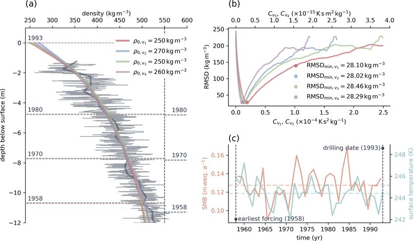
T. Schultz et al.: Assessment of a grain boundary sliding model for firn densification                                               145

that the effect of grain boundary sliding on the strain rate de-      Variant 1 (Eq. 2) and Variant 2 (Eq. 3) of the constitutive
creases, whereas that of other processes increases. The stud-         equation combine all material constants using the factors Cv1
ies of Arthern and Wingham (1998) and Bréant et al. (2017)            and Cv2 , respectively. The Arrhenius factor for boundary
use this description, in which only grain boundary sliding            diffusion, DBD (see Eq. 1), is retained in these variants.
drives densification in the first stage of firn densification. In     Following Maeno and Ebinuma (1983), we use a value of
the study of Bréant et al. (2017), the constitutive relation of       QBD = 44.1 kJ mol−1 for the boundary diffusion activation
Alley (1987) is changed such that the transition into the sec-        energy. This variable was defined by Maeno and Ebinuma
ond stage of densification is modified. We evaluate this mod-         (1983) as two-thirds of the activation energy for lattice dif-
ification in this work.                                               fusion measured by Itagaki (1964). The corresponding pref-
   Finally, the stress in the vertical direction, σzz , result-       actor is ABD = 3.0 × 10⁻² m2 s−1 . Alley (1987) assumed a
ing from the overburden firn drives grain boundary sliding.           similar value for the boundary diffusion activation energy.
Whereas Alley (1987) used the product of the accumulation                 In addition to the temperature T , the vertical strain rate ε̇zz
rate, acceleration due to gravity, and time since the deposition      depends only on the firn density ρ, grain radius r, and stress
of a specific firn sample to describe the overburden stress, we       in the vertical direction σzz . Variant 2 differs from Vari-
use a more general form here (see Sect. A2, Eq. A5). The              ant 1 in that it uses the modification introduced by Bréant
other physical properties affecting the process are density ρ,        et al. (2017). This modification causes a theoretical end to
temperature T , and grain radius r.                                   the process of grain boundary sliding at a density of ρc∗ =
                                                                      596 kg m−3 . It was introduced to obtain a better transition to
2.2       Optimization                                                the second stage of firn densification. The strain rate due to
                                                                      grain boundary sliding is therefore higher at the critical den-
To test the material model developed by Alley (1987), we for-         sity when this modification of Bréant et al. (2017) is used.
mulated variants of Eq. (1) and compared the model results                To determine the effect of the Arrhenius factor, it is disre-
to density measurements of various firn cores. These variants         garded in variants 3 and 4, as shown in Eqs. (4) and (5):
of the constitutive Eqs. (2) to (5) preserve its general form
but group several material parameters into a single factor. As                         1 1 ρice 3

                                                                                                         5 ρ
a result, the simulation result does not depend on those pa-          ε̇zz v3 = −Cv3                 1−            σzz ,              (4)
                                                                                      T r ρ              3 ρice
rameters but on the single factor. The factor is then varied
                                                                                       1 1 ρice 3

to find an optimal simulation result that best reproduces the                                            0.5 5 ρ
                                                                      ε̇zz v4 = −Cv4                 1+        −           σzz .      (5)
measured firn profile. The factor that yields the optimal sim-                        T r ρ                6      3 ρice
ulation result depends on the measured firn density profile           In Variant 4, the modification of Bréant et al. (2017) is used,
and the corresponding climate conditions. It is therefore site-       whereas Variant 3 uses the original formulation of Alley
specific. This feature makes it possible to assess whether the        (1987). The goal of the optimization is to find optimal val-
description of grain boundary sliding given by Alley (1987)           ues of the factors Cv for every variant of the constitutive
can be used to reproduce measured firn profiles, assuming an          relation (Eqs. 2 to 5) to produce simulated density profiles
optimal set of parameters. It further allows us to analyze the        that best reproduce the measured profiles. As an example,
site-specific factors yielding the best simulation results for        we explain the optimization process for one selected firn core
possible hidden dependencies.                                         in more detail. The upper part of ice core ngt03C93.2 (Wil-
   Arnaud et al. (2000), Goujon et al. (2003), and Bréant             helms, 2000) is shown in Fig. 1a.
et al. (2017) also incorporated the material parameters of the           Every simulation begins with a spin-up period in which
model of Alley (1987) into a single parameter. Bréant et al.          constant values are used for forcing. The model is forced
(2017) also modified the factor of 5/3 to change the density          with prescribed values of temperature, accumulation rate,
at which the deformation due to grain boundary sliding be-            firn density, and grain radius at the surface. We check for
comes zero. In the following, four variants, indicated by the         steady-state conditions by comparing the change in den-
subscripts (·)v1 to (·)v4 , are presented:                            sity between time steps. If the maximum density change
                                                                      is smaller than |1ρmax | < 0.1 kg m−3 , we assume that the
                       1 1 ρice 3

                                         5 ρ                          steady state is reached. In this case, a transient run using
ε̇zz v1 = − Cv1 DBD                1−             σzz ,
                       T r ρ             3 ρice                       varying forcing data follows. We use a constant value of 48
                                                                      time steps per year for spin-up and transient simulation runs

                              QBD
            DBD = ABD exp −          ,                          (2)   (see Sect. A7). The forcing at the location of ngt03C93.2
                               RT
                                                                      is shown in Fig. 1c. The resulting firn profile is then com-
                      1 1 ρice 3

                                       0.5 5 ρ
ε̇zz v2   = − Cv2 DBD             1+       −            σzz ,         pared to the measured profile. We used the root mean square
                      T r ρ             6     3 ρice                  deviation (RMSD) between the measured and modeled den-

                             QBD                                      sity for comparison, as it is simple and easy to compute. To
           DBD = ABD exp −         .                            (3)
                              RT                                      calculate the deviation, the simulated density values are in-
                                                                      terpolated linearly to the measurement locations along the

https://doi.org/10.5194/tc-16-143-2022                                                          The Cryosphere, 16, 143–158, 2022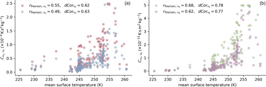
146                                     T. Schultz et al.: Assessment of a grain boundary sliding model for firn densification

Figure 1. (a) Depth density profile of ice core ngt03C93.2 (Wilhelms, 2000) retrieved in Greenland (gray) and best corresponding model
results obtained using four variants of constitutive law for grain boundary sliding of Alley (1987) (various colors). Dark gray line shows
the mean density of the ice core calculated using a window of 0.5 m starting at the surface. Dashed horizontal lines represent horizons
of firn deposited in the indicated years, where 1958 is the first year that forcing from RACMO2.3 (Van Wessem et al., 2014; Noël et al.,
2015) is available. Colored dashed horizontal lines show horizons obtained in the simulations. Horizons plotted in gray (to the right of the
vertical dashed line) represent the same surfaces as those determined by Miller and Schwager (2004) during analysis of the core. (b) RMSD
between measured and modeled density plotted over the range of tested factor values. Note the different axes for different tested factors.
(c) Representative forcing at the location of ice core ngt03C93.2, which was used in the simulation. Horizontal dashed lines show the mean
values of the surface mass balance and surface temperature during the simulation.

profile. To ensure the quality of the results, we limited the           of 540 kg m−3 was chosen to ensure that the results obtained
calculation of the deviation to the domain defined by the               using the variants of the constitutive relation are comparable,
location of the uppermost available measurement point and               whereas unique values of the factor Cv were quickly deter-
the oldest simulated horizon within the firn profile affected           mined throughout the optimization.
by forcing. For ngt03C93.2, this horizon is the 1958 surface               As the implementation of our model is efficient and the
at a depth of approximately 11 m below the surface, indi-               approach is simple and reliable, we decided to determine
cated by dashed horizontal lines in Fig. 1a. Only results lo-           the best factor Cv for the four variants of the constitutive
cated above the simulated 1958 surface are used to calcu-               equation by simply testing 250 values within certain ranges.
late the deviation. The reason is that the forcing data from            These ranges are shown in Eqs. (6) and (7), which include
RACMO2.3 (Van Wessem et al., 2014; Noël et al., 2015) be-               and exclude the Arrhenius factor, respectively. Optimal fac-
gin in 1958 for Greenland. Consequently, the results are not            tors can be found within these ranges for every analyzed firn
affected by the spin-up period. For firn profiles retrieved in          profile. To ensure that this is the case, all simulations were
Antarctica, climate forcing from RACMO2.3 begins in 1979.               performed multiple times using different ranges of the fac-
Thus, only those results located above the simulated hori-              tors.
zon of 1979 are considered for comparison with the Antarc-
tic firn profiles. The examination of other firn cores revealed         1.0 × 10⁻⁹ K s2 kg−1 ≤ Cv1 ,v2 ≤ 2.5 × 10⁻⁴ K s2 kg−1           (6)
that the surface of the oldest available forcing may be lo-             2.5 × 10⁻²¹ K s m2 kg−1 ≤ Cv3 ,v4 ≤ 5.0 × 10⁻¹⁵ K s m2 kg−1 (7)
cated at greater depth when the density of ρc = 550 kg m−3
                                                                        Figure 1b shows the RMSD plotted over the 250 tested values
has already been reached. In those cases, the computation of
                                                                        for the four different factors. The variants are color-coded,
the RMSD was limited to the domain showing density val-
                                                                        and the best results are marked. The smallest values of the
ues below 540 kg m−3 . We decided to use a density thresh-
                                                                        deviation are shown in the figure. The corresponding density
old below the critical density because of the asymptotic na-
                                                                        profiles are shown in Fig. 1a.
ture of the resulting density profiles obtained using variants 1
                                                                           The firn profile of ngt03C93.2 starts at a depth of ap-
and 3 of the constitutive equation (Eqs. 2 and 4). The value
                                                                        proximately 1.3 m. Therefore, an appropriate surface density

The Cryosphere, 16, 143–158, 2022                                                              https://doi.org/10.5194/tc-16-143-2022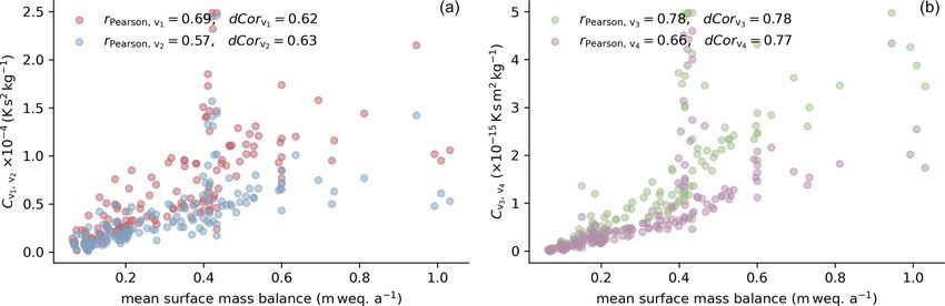
T. Schultz et al.: Assessment of a grain boundary sliding model for firn densification 147
boundary condition must be found. As firn density profiles mass balance should be positive, as stated in the fifth crite-
differ greatly, especially near the surface, the derivation of rion. However, a positive mean annual surface mass balance
an appropriate surface density is difficult. Although Alley does not ensure that no melting occurs over the course of a
(1987) simulated the density starting at a depth of 2 m below year. It is not possible to distinguish between sites affected
the surface, we included this domain in our simulation so by melting and sites where no melting occurs using the data
that we could apply transient surface forcing to our model. available for this study. The number of these sites, however,
To find suitable values of the surface density, we included is expected to be small. Because of the method used, their
this parameter in our optimization. For each of the four vari- influence on the overall result is therefore small. The forc-
ants and 250 factors Cv , we tested 21 values of the surface ing data come from the regional climate model RACMO2.3
density between ρ0 = 250 and ρ0 = 450 kg m−3 , using steps (Van Wessem et al., 2014; Noël et al., 2015), which pro-
of 1ρ0 = 10 kg m−3 . The best result was chosen. We used vides the surface mass balance. The model delivers data for
the method of testing 21 surface density values for all the the periods 1958 to 2016 and 1979 to 2016 for Greenland
analyzed firn profiles. We included profiles including mea- and Antarctica, respectively (see also Sect. 3.2). The density
surements of the density at small depths. In this way, we es- measurements used for model comparison should thus be re-
tablished that the results are comparable. Profiles including trieved during these periods. We used only datasets for which
near-surface density values are, however, well represented. at least 5 years of forcing data are available. Furthermore, a
A total of 4×250×21 = 21 000 simulations were performed number of density profiles were manually excluded from the
for ice core ngt03C93.2 to find the optimal results shown in filtered data. These profiles include those with very low spa-
Fig. 1. The same procedure was applied to all 159 firn pro- tial resolution, atypical profiles showing decreasing density
files analyzed in the study. with depth, and measurements with a surface density very
close to the critical density of ρc = 550 kg m−3 . As explained
in Sect. 2.2 and illustrated in Fig. 1, we used only a certain
3 Data domain for the comparison of the simulated and measured
data. If this domain was found to be less than 2.5 m long for
3.1 Firn profiles
any of the tested variants of the constitutive equation, the firn
To evaluate the description of grain boundary sliding given profile in question was not analyzed further.
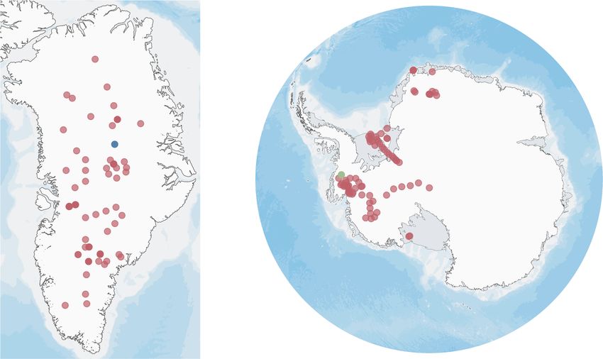
by Alley (1987), we used 159 firn profiles, 80 of which Figure 2 shows the locations from which the 159 density
were retrieved in Greenland. The remaining 79 measure- profiles were retrieved. The 80 measurements from Green-
ments were taken in Antarctica. The profiles are included land are relatively uniformly distributed over the ice sheet.
in the SUMup snow density subdataset (Koenig and Mont- Coastal locations are not well covered owing to the re-
gomery, 2019). Individual references for all 159 firn profiles quirement of a strictly positive surface mass balance. In
are listed in the Supplement. The dataset does not include the the Antarctic, sites in East Antarctica are underrepresented.
four profiles used in the study of Alley (1987), as the orig- However, a wide variety of environments is covered, includ-
inal data for these firn cores are unpublished. To obtain firn ing the Filchner–Ronne Ice Shelf, the West Antarctic coast,
profiles suitable for this study from the dataset, we filtered it and Dronning Maud Land.
according to the following criteria.
3.2 Boundary conditions and forcing
1. Profiles must consist of at least 10 data points.
To force the firn densification model, we need the surface
2. The overall length of each profile must exceed 3 m. values of density, temperature, accumulation rate, and grain
3. Profiles must start at a depth of less than 3 m below the radius at the locations of the 159 firn profiles. Although Alley
surface. (1987) used constant forcing, we followed the example of
Arthern and Wingham (1998) and Goujon et al. (2003), who
4. The initial density of the profiles must not exceed ρc = performed transient simulations.
550 kg m−3 . As measured firn density profiles represent past climate
conditions, the choice of forcing data in the proposed method
5. The annual mean surface mass balance at the profile lo- is crucial. Uncertainties in the forcing will affect the sim-
cations must be strictly positive. ulation results and therefore the comparison with the mea-
6. Forcing data for at least 5 years must be available for sured firn profiles. Neither the model formulation nor the op-
the profile location. timization scheme can compensate for these effects. We used
data provided by the regional climate model RACMO2.3
Criteria 1 and 2 ensure the overall quality of the data, (Van Wessem et al., 2014; Noël et al., 2015). Details on
whereas criteria 3 and 4 ensure that the first stage of firn den- RACMO2.3, including the limitations of the model and the
sification is included. As the model cannot handle melting resulting data products, were presented by Van Wessem et al.
and the study focuses on dry firn densification, the surface (2014), Noël et al. (2015), and van Wessem et al. (2018).
https://doi.org/10.5194/tc-16-143-2022 The Cryosphere, 16, 143–158, 2022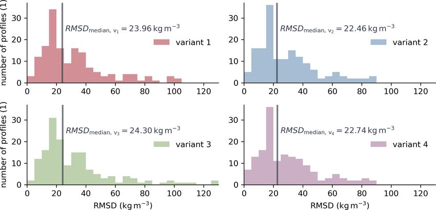
148                                     T. Schultz et al.: Assessment of a grain boundary sliding model for firn densification

                                                                     fied using the optimization approach. The results obtained
                                                                     using the annually averaged forcing data are shown on the
                                                                     left, whereas those obtained using monthly averaged data
                                                                     from ERA5 are shown on the right. The data with higher tem-
                                                                     poral resolution reveal much more detail within the simulated
                                                                     firn density profiles. However, the aim of this study is not
                                                                     primarily to reproduce the analyzed measured firn profiles
                                                                     with the highest possible detail but to evaluate the constitu-
                                                                     tive relation of Alley (1987) using an optimization approach
                                                                     that identifies site-specific optimal constitutive factors Cv
                                                                     (see Sect. 2.2). Figure 3b shows the RMSD of the simulated
                                                                     profiles from the measured profile over the range of tested
                                                                     optimization factors. Dashed lines represent simulations per-
Figure 2. Locations of firn profiles used for model comparison.      formed using the high-resolution forcing data, whereas solid
Eighty profiles were measured in Greenland, and 79 depth den-
                                                                     lines represent the annual averaged data. The difference be-
sity datasets were retrieved in Antarctica. The blue marker shows
                                                                     tween the optimization results is small. We therefore used
the location of ice core ngt03C93.2 (Wilhelms, 2000, 73.940◦ N,
−37.630 ◦ E). The green marker shows the location of site 3 of the   the annual averaged data provided by RACMO2.3 suitable
iSTAR traverse, from which the firn core shown in Fig. 3 was re-     for this study, as the data cover a longer time period, espe-
trieved (Morris et al., 2017, −74.565◦ N, −86.913◦ E). Map data:     cially for Greenland. As a result, we can analyze more firn
Amante and Eakins (2009) and Arndt et al. (2013), SCAR Antarctic     profiles at greater detail. For ice core ngt03C93.2 (Wilhelms,
Digital Database.                                                    2000), the horizon of the year 1981, the earliest forcing avail-
                                                                     able in ERA5, lies at a depth of approximately 5 m below the
                                                                     surface, as shown in Fig. 1a. The horizon of the earliest forc-
RACMO2.3 provides forcing data for the Greenland ice sheet           ing available from RACMO2.3, the year 1958, is located at
covering 1958 to 2016. For Antarctica, the time period is            a depth of approximately 11 m below the surface. A much
shorter, running from 1979 to 2016. Data for the mean annual         greater portion of the simulated firn profile is therefore af-
skin temperature and surface mass balance of the Greenland           fected by surface forcing. Furthermore, the use of yearly av-
ice sheet are available at mean spatial resolutions of 11.3 and      eraged data requires less overhead.
1.0 km, respectively, for this study. The mean spatial resolu-          As noted in Sect. 2.2, we used 21 surface density values in
tions of the mean annual skin temperature and surface mass           the range 250 kg m−3 ≤ ρ0 ≤ 450 kg m−3 for every tested firn
balance for Antarctica are 8.0 and 28.5 km, respectively.            profile. The value that yielded the best result was then used
   The time period for the transient simulation runs, as de-         for further analysis. Owing to a lack of relevant data, and
scribed in Sect. 2.2, is specified by the earliest data available    for simplicity and ease of comparison, the grain radius at the
from RACMO2.3 and the drilling date of the firn core under           surface was assumed to be the same at all locations and to be
consideration. For ice core ngt03C93.2 (Wilhelms, 2000),             constant over time. We used a grain radius of r0 = 0.5 mm
which was retrieved in central Greenland in 1993, the simu-          on the basis of the measurements and empirical relation of
lation time covers the period from 1958 to 1993 (see Fig. 1c).       Linow et al. (2017) and the assumption of Arthern and Wing-
Constant values of the surface temperature and surface mass          ham (1998). As climatic conditions, and therefore the surface
balance for the preceding spin-up period were calculated as          grain size, vary among the investigated locations, this choice
mean values over this time range.                                    is a simplification. Owing to the use of the optimization ap-
   We present a second example to illustrate the effect of           proach, this parameter has a less significant effect, as it can
the temporal resolution of the forcing on the optimization           be understood as a constant part of the grain radius, which is
results and why we used yearly averaged data provided by             the same for every analyzed firn profile.
RACMO2.3. Figure 3 shows the depth density profile of the               Figure 4 illustrates the range and distribution of surface
firn core retrieved at site 3 of the iSTAR Traverse in 2013          boundary conditions at the investigated sites. The locations
(Morris et al., 2017). The location of the site, at Pine Island      in Greenland show a higher mean surface temperature and
Glacier in West Antarctica, is shown in Fig. 2. Instead of us-       surface mass balance than those in Antarctica. The surface
ing forcing data from RACMO2.3, for this particular simula-          density is higher at the Antarctic locations than at those in
tion we used ERA5-Land monthly averaged data from 1981               Greenland. Overall, a wide variety of typical climatic condi-
to present (Muñoz Sabater, 2019; Hersbach et al., 2020), as          tions for both ice sheets is covered.
they are freely available at monthly resolution. From these
data, we computed the annual average data for a second sim-          3.3   Distribution and effects of input data
ulation run. The forcing data at both resolutions are shown in
Fig. 3c. Figure 3a shows the simulated firn profiles that best       Ice core ngt03C93.2 (Fig. 1a) is an example of a high-
reproduce the measured density profile, which were identi-           resolution density measurement showing extensive small-

The Cryosphere, 16, 143–158, 2022                                                         https://doi.org/10.5194/tc-16-143-2022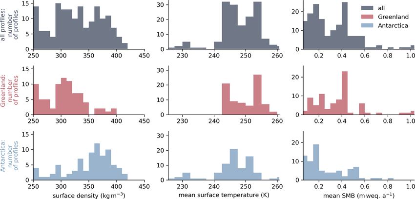
T. Schultz et al.: Assessment of a grain boundary sliding model for firn densification                                                     149

Figure 3. (a) Depth density profile (gray) of the firn core retrieved at site 3 of the iSTAR traverse (Morris et al., 2017). Colored lines show
the optimal simulation results for four tested variants of the constitutive relation. The simulated density profiles on the left were obtained
using yearly averaged surface forcing, whereas those on the right, plotted using dashed lines, were obtained using monthly averaged forcing.
(b) RMSD between best simulation result and measured firn profile over the range of tested optimization factors Cv . Colors indicate results
for the different variants of the constitutive relation. Dashed lines indicate results computed with monthly averaged forcing, whereas solid
lines indicate the use of yearly averaged surface forcing. (c) Forcing data from ERA5-Land monthly averaged data from 1981 to the present
(Muñoz Sabater, 2019; Hersbach et al., 2020), from the earliest available forcing in 1981 to the date the firn core was drilled in 2013. Bold
lines show yearly averaged data computed from monthly averaged data.

Figure 4. Distribution and comparison of boundary conditions at the 159 firn profile sites. All values are averaged over the simulation time for
each location, beginning in 1958 and 1979 for Greenland and Antarctica, respectively, and ending at the date of measurement (see Sect. 3.2).
The top row of plots (gray) shows the boundary conditions at all locations, whereas the middle and bottom rows, in red and blue, show only
the locations in Greenland and Antarctica, respectively. Data for the surface temperature (center) and surface mass balance (right column)
are provided by RACMO2.3 (Van Wessem et al., 2014; Noël et al., 2015).

scale layering. Only a few of the 159 firn profiles are of such           ris et al., 2017) (Fig. 3) illustrates that the model, if it is
high quality and include this type of layering. Although our              forced with data of higher temporal resolution, still does not
proposed model works at high temporal and spatial resolu-                 cover the measured density variability. Small-scale layering
tion, it does not cover layering, as shown in Fig. 1a. The den-           of firn appears to be driven by a number of different pro-
sity profile retrieved at site 3 of the iSTAR traverse (Mor-              cesses (Hörhold et al., 2011). An extension of the model to

https://doi.org/10.5194/tc-16-143-2022                                                               The Cryosphere, 16, 143–158, 2022
150                                     T. Schultz et al.: Assessment of a grain boundary sliding model for firn densification

Figure 5. Distribution of smallest RMSD for every analyzed firn profile found using the optimization scheme outlined in Sect. 2.2. The four
plots show the results for the four tested variants of the constitutive equation. Vertical lines indicate the median of the 159 values.

cover such processes may be introduced in the future. We                yields a value of 1Cv1 ,max = 0.02 × 10⁻⁴ K s2 kg−1 , which
would prefer the approach of Freitag et al. (2013), who intro-          corresponds to twice the sampling space of the factors Cv1
duced the concept of impurity-controlled densification. Forc-           used in the optimization. Variant 4 yields the same results.
ing data for this model are not globally available. However,            Because of this small effect overall, the stronger effect of the
the model in its current form does reproduce the mean den-              surface temperature in the investigated domain, and the lim-
sity well, as demonstrated in Fig. 1a.                                  itation of the comparison to the domain actually affected by
   In this study, we focused on the initial stage of firn densifi-      surface forcing, a Neumann boundary condition at the profile
cation and the uppermost part of the firn column. We limited            base is justified despite the low depth.
the model domain to a maximum depth of −25 m below the
surface. Furthermore, we did not develop the density further
after the critical density of ρc = 550 kg m−3 was reached.              4   Results
This choice raises the question of whether the use of a Neu-
mann boundary condition set to zero at the profile base to              Figure 5 shows the distribution of the RMSD calculated from
solve for the temperature is justified for this particular model        the simulated firn profiles that best reproduce the measured
setup (Sect. A4). The critical density of ρc = 550 kg m−3 is            profiles. The four plots in the figure represent the four vari-
usually reached within the upper 10 m of the firn column.               ants of the constitutive equation for grain boundary sliding
The temperature within this domain is affected by surface               (Eqs. 2 to 5), as described in Sect. 2.2. Additionally, the me-
conditions, which are covered by the forcing data. At greater           dian values of the data are shown. The distributions of the
depths, the temperature corresponds to the mean annual sur-             deviation for the four variants show little difference. The me-
face temperature and changes very little (e.g., Cuffey and Pa-          dian values differ in a small range. Variants 2 and 3 show
terson, 2010, 399 pp.). There have been few high-resolution             the smallest and largest values, respectively. The use of the
temperature measurements of firn. Orsi et al. (2017) pub-               modification introduced by Bréant et al. (2017) in the con-
lished a temperature profile of a 147 m length from bore-               stitutive equation improves the agreement between the sim-
hole NEEM2009S1, which shows a temperature difference                   ulated and measured firn profiles by 6.2 %–6.8 %. To put the
of little more than 1 K over the entire profile. Vandecrux              values in perspective, the deviation of the four best-fitting
et al. (2021) obtained the same result. This small tempera-             modeled firn profiles from ice core ngt03C93.2 (Wilhelms,
ture change at depths greater than approximately 10 m below             2000) displayed in Fig. 1 is approximately 28 kg m−3 . That
the surface has little effect on our model approach. To test            is, more than half of the simulations show even better agree-
the temperature dependence of the optimization approach,                ment with the corresponding firn density profiles than this
we performed the simulations again using the site-specific              one. An overview of the deviation among all 159 measured
surface temperature forcing plus or minus 1 K. The effect on            firn profiles and the corresponding best simulation results can
the optimal factors Cv depends on the variant of the con-               be found in the Supplement.
stitutive relation, but it is generally small. For example, the            The range of factors contributing to the best-fitting firn
greatest difference between the optimal factors obtained us-            profile is smaller for variants 2 and 4 of the constitutive equa-
ing the correct and adjusted forcing for ice core ngt03C93.2            tion, which use the modification of Bréant et al. (2017), com-
(Wilhelms, 2000) were found using Variant 1. This variant               pared to variants 1 and 3, as shown in the box plots in Fig. 6.
                                                                        In contrast to factors Cv1 and Cv2 , factors Cv3 and Cv4 incor-

The Cryosphere, 16, 143–158, 2022                                                             https://doi.org/10.5194/tc-16-143-2022
T. Schultz et al.: Assessment of a grain boundary sliding model for firn densification 151
order function, as indicated by the higher values of the dis-
tance correlation.
The values of the Pearson correlation coefficient and dis-
tance correlation shown in Fig. 8, which shows the factors
with respect to mean surface mass balance, are higher than
those in Fig. 7.
Like the mean surface temperature, the mean surface mass
balance was calculated from the forcing data used during the
simulations. The correlation coefficients for the results ob-
tained using variants 3 and 4 exceed those for the results
Figure 6. Box plots showing the distribution of the best factors, Cv1 obtained using the variants of the constitutive equation in-
to Cv4 , for the four variants of the constitutive equation describing corporating the Arrhenius factor explicitly. Variant 3 shows
grain boundary sliding (Eqs. 2 to 5) derived using the optimization the best indication of a relationship between surface mass
scheme described in Sect. 2.2. The quartile coefficient of disper- balance and the factor yielding the density profile that best
sion vr of each variant is shown on the right in the corresponding reproduces the corresponding field measurement.
color. The quartile coefficient of dispersion was calculated using the In Fig. 8, a striking feature appears around a mean sur-
first (Q1 ) and third (Q3 ) quartile values of the datasets, which are face mass balance of 0.4 m weq. a−1 . The values of the fac-
shown in black and represent a robust relative measure of disper-
tors yielding the simulated density profiles that best repro-
sion.
duce the measured profiles show a wide range for all four
variants of the constitutive relation. These profiles are part of
a study in western Greenland by Harper et al. (2012). The
study region is relatively small, which explains the similar
porate the Arrhenius factor from the original description of climatic conditions. Although the mean annual surface mass
grain boundary sliding given by Alley (1987). Therefore, di- balance is positive, melting occurs throughout the year and
rect comparison between the two groups of factors is not pos- affects the firn density.
sible. The quartile coefficient of dispersion of the four vari-
ants, which is shown on the right side of Fig. 6, is a relative
measure of the scatter of the values. The coefficient reveals 5 Discussion
that the factors obtained for variants 1 and 2 are defined in a
narrower range than those of variants 3 and 4. All four sets Using the four variants of the constitutive relation of Al-
of factors show slightly nonuniform distributions that tend ley (1987) (Eqs. 2 to 5), we generated density profiles that
toward smaller values. were in good agreement with most of the 159 density mea-
To check for possible mean surface temperature depen- surements. Uncertainties may result from the forcing, limited
dence of the 159 factors found by optimization, these values knowledge of the initial grain radius, and the poor constraint
are plotted against each other in Fig. 7. The values of the on the density at the surface. As measured firn densities rep-
mean surface temperature were calculated from the forcing resent past climate conditions, unrealistic forcing always re-
data for each firn profile site. The left plot illustrates the re- sults in a mismatch between the simulated and measured
sults for variants 1 and 2 in red and blue, whereas the right firn properties, independent of the optimization approach and
plot shows the factors for variants 3 and 4 using green and physical model. However, when the proposed optimization
purple markers, respectively. The legend shows the Pearson scheme was used, the differences between the simulated and
correlation coefficient rPearson , a measure of the linear corre- measured density profiles show distinct minima, indicating
lation of the two variables, and the distance correlation dCor that the forcing represents the climatic history of the firn pro-
(Székely et al., 2007). The distance correlation was designed files, in principle.
by Székely et al. (2007) to overcome problems with the Pear- The optimization scheme produces site-specific values of
son correlation coefficient. It describes the correlation of two the factors Cv1 to Cv4 . As the optimization process is unique
vectors and is not limited to linear dependence. It is defined to each analyzed site and constitutive relation variant, the
between zero and one, where zero indicates the independence four simulated density profiles for each site are very simi-
of the variables. lar, as illustrated in Fig. 5. This feature allows us to compare
The correlation between the resulting factors and the mean the factors obtained using the four variants. The differences
surface temperature is higher compared to the correlation between the factors do not arise primarily from differences
with other properties. This statement is especially true for in the simulated density profiles but reflect the differences in
factors Cv3 and Cv4 of variants 3 and 4, respectively. How- the variants; consequently, the results are almost the same.
ever, the Pearson correlation coefficient indicates only a lin- However, owing to the nature of the optimization scheme,
ear correlation. The scatter of factors Cv3 and Cv4 with re- possible errors in the forcing data or other parameters such
spect to mean surface temperature might resemble a higher- as the activation energy used to calculate the grain radius
https://doi.org/10.5194/tc-16-143-2022 The Cryosphere, 16, 143–158, 2022152 T. Schultz et al.: Assessment of a grain boundary sliding model for firn densification
Figure 7. Best factors for every investigated firn profile determined using the optimization scheme and plotted against mean surface temper-
ature during forcing period (see Sect. 4). (a) Results for variants 1 and 2 of the constitutive equation in blue and red, respectively. (b) Results
for variants 3 and 4 in green and purple, respectively. The Pearson correlation coefficient rPearson , which represents the linear correlation
between factors Cv1 to Cv4 and the mean surface temperature, as well as the distance correlation dCor, is given in the legend.
Figure 8. Factors obtained by optimization versus mean surface mass balance, calculated for 159 firn profiles from the forcing. (a) Best-fitting
values for variants 1 and 2 (factors Cv1 and Cv2 , respectively). (b) Best-fitting values for variants 3 and 4 (factors Cv3 and Cv4 , respectively).
Linear correlation between the factors and mean surface mass balance is indicated by the Pearson correlation coefficient rPearson , and the
general correlation is indicated by the distance correlation dCor.
(see Eq. A11) are also included in the site-specific optimal part of the firn body (e.g., Vandecrux et al., 2020). The pro-
factors Cv1 to Cv4 . If, for example, the surface tempera- posed method could be improved by the application of this
ture forcing at a site consistently deviates by 5 K during the model approach in future investigations. However, we iden-
simulation, this error can be compensated for by adjusting tified some correlations between the optimization results and
the specific optimization factor Cv (see Sect. 3.3). However, the surface mass balance.
the large number of analyzed firn profiles compensates for Note, again, that we have not investigated whether grain
such random errors. Systematic errors in the forcing data boundary sliding is indeed the dominant process during the
(van Wessem et al., 2018) cannot be identified. Therefore, first stage of firn densification. We assess whether a pro-
improving the temporal resolution of the forcing and cover- cess with a functional dependence on density, firn overbur-
ing longer periods could result in better and more detailed den stress, temperature, and grain radius represents the ob-
simulation results, as shown in Fig. 3. served density profiles well. Any other deformation process
This study analyzed only dry firn densification. The cur- with the same functional dependence would be equally well
rent model cannot handle melting. We accommodate this fea- suited. Nevertheless, by maintaining the general structure of
ture by setting the annual mean surface mass balance at the the constitutive relation of Alley (1987), we conclude that
investigated sites to be strictly positive (Sect. 3.1). However, this description of grain boundary sliding is a good basis for
this limitation means that we cannot ensure that no melt- a physically based model describing firn densification up to
ing occurs over the course of a year. The results shown in the critical density, ρc = 550 kg m−3 .
Fig. 8 illustrate how this limitation affects the optimization Comparing the results for variants 1 and 2, as well as
results. The limitation is problematic, especially in recent those
for variants
3 and 4, we found that an adjustment of
years, when melting occurred over almost the entire Green- 1 − 3 ρ/ρice to 1 + 0.5
5 5
6 − 3 ρ/ρice results in better repro-
land ice sheet (e.g., Nghiem et al., 2012). The simulation duction of the measured density profiles. This result must
of meltwater percolation through the firn and its interaction be reviewed carefully in terms of the study design and the
with firn densification is important, especially in the upper background of a physics-based model describing firn densi-
The Cryosphere, 16, 143–158, 2022 https://doi.org/10.5194/tc-16-143-2022T. Schultz et al.: Assessment of a grain boundary sliding model for firn densification 153
fication. As Alley (1987) pointed out, grain boundary sliding tal direction. The horizontal components of the stress tensor
might be the dominant process driving firn densification at are not zero. As firn is a compressible material, the deter-
low densities, but it is presumably not the only one. The con- mination of these horizontal stress components is not trivial.
stitutive law of Alley (1987) is designed such that the den- The frequently used term “overburden pressure” is mislead-
sification due to grain boundary sliding becomes zero at a ing, as the mechanical pressure is defined as the spherical
density of ρc = 550 kg m−3 , owing to the densest packing part of the Cauchy stress tensor (e.g., Haupt, 2002, p. 301)
of spheres obtained at that density and increasing accom- and is not, in general, identical to the normal stress in the
modation incompatibilities. The modification of Bréant et al. vertical direction. With increasing depth, the magnitude of
(2017) changes this behavior such that grain boundary slid- the horizontal stress components and their effects would in-
ing vanishes at a density of approximately ρc∗ = 596 kg m−3 , crease. Modeling approaches that consider the full stress ten-
which could have advantages for the transition into the next sor were reported by Greve and Blatter (2009), Salamantin
stage of firn densification. We suggest that a simultaneous et al. (2009), and Meyer and Hewitt (2017). It might be worth
decrease in grain boundary sliding and increase in one or using the constitutive relation for grain boundary sliding of
more other processes would provide a good characterization. Alley (1987) in such a modeling context. This approach will
Specifically, dislocation creep drives densification at higher not necessarily result in a full three-dimensional model, as
density (Maeno and Ebinuma, 1983) because of increasing the problem can be formulated assuming axial symmetry,
stresses. The onset of dislocation creep at densities below which would require adjustment of the constitutive relation.
ρc = 550 kg m−3 would not necessarily affect the entire bulk A more extensive interpretation of the factors that yielded
firn matrix but increasing volume fractions of the porous ma- the best agreement is therefore challenging. The determina-
trix. tion of a single factor Cv for one or all of the variants is
Variants 1 and 2 of the constitutive relation of Alley not useful. It would not result in better simulation results
(1987) incorporate the Arrhenius factor for boundary diffu- compared to other published firn densification models. The
sion, DBD , from the description of the bond viscosity given site-specific values of the factors determined using the pre-
by Raj and Ashby (1971). In the formulation of variants 3 sented optimization approach simply show the differences in
and 4, we neglected the Arrhenius factor. As shown in Fig. 5, the variants of the constitutive relation.
the difference in the resulting RMSD is small regardless of
whether DBD is considered. This result is reasonable, as we
determined individual factors Cv for each site. The similarity 6 Conclusions
of the results allows us to compare the factors Cv1 and Cv2 ,
Using variants of the constitutive relation for grain bound-
which were determined using the Arrhenius factor DBD , to
ary sliding of Alley (1987) and an efficient optimization
factors Cv3 and Cv4 , which were obtained using the variants
scheme, we reproduced 159 firn density profiles reasonably
of the constitutive relation without the Arrhenius factor. As
well. Thus, we conclude that the description of grain bound-
DBD is a function of temperature, it is reasonable to examine
ary sliding introduced by Alley (1987) is appropriate for the
the dependence of the factors on the mean surface tempera-
simulation of firn densification at low density.
ture, which is shown in Fig. 7.
The modification of the constitutive relation of Bréant
The factors Cv3 and Cv4 , which were determined using the
et al. (2017) results in slightly better simulation results when
variants without DBD , show a stronger dependence on the
only the first stage of firn densification is considered. Further
mean surface temperature than the factors Cv1 and Cv2 . In ad-
factors, including the transition from the first to the second
dition, the factors Cv1 and Cv2 show less dispersion than Cv3
stage, must be considered to answer questions regarding in
and Cv4 , as shown in Fig. 6. The inclusion of DBD in the con-
which domain and to what extent different processes drive
stitutive relation improves the determination of these factors.
firn densification.
It is therefore a meaningful description within the constitu-
In our optimization approach, we use a single factor rep-
tive relation. Although the inclusion of the Arrhenius factor
resenting various model parameters and search for the factor
improves the determination of Cv1 and Cv2 , we still see some
value resulting in the best agreement between the simulated
dependence on the mean surface temperature. A better de-
and measured firn profiles. Consequently, the site-specific
termination of the parameters of the Arrhenius factor may
simulation results are independent of the possibly deficient
resolve this dependence. If this is not the case, another de-
model parameters, which are considered collectively. It is not
pendence on the temperature may be introduced to improve
possible to derive a distinct value for the factor representing
the constitutive relation for grain boundary sliding.
the climatic conditions at all locations of the investigated firn
We interpret the dependence on surface mass balance as
profiles. We found a linear dependence of the factors on the
indicating that the load is currently not represented well. The
site-specific surface mass balance (Fig. 8). By contrast, we
stress is represented by a second-order tensor. A firn col-
did not find a clear linear dependence on temperature (Fig. 7),
umn represented by a one-dimensional modeling approach
but the results show that a site-specific parameter is required.
would be surrounded by neighboring firn columns, resulting
in lateral confinement that limits deformation in the horizon-
https://doi.org/10.5194/tc-16-143-2022 The Cryosphere, 16, 143–158, 2022154 T. Schultz et al.: Assessment of a grain boundary sliding model for firn densification
As the amount of surface accumulation affects the load
conditions, we assume it is not represented well in the model.
Unlike other firn densification models, the physical simula-
tion of grain boundary sliding does not depend directly on
the surface mass balance but depends on the actual stress.
Further interpretation of the obtained factors is difficult us-
ing the presented simulation setup. The description of grain
boundary sliding given by Alley (1987) could be improved
by using a higher-dimensional approach including the hori-
zontal components of the stress tensor. Modeling approaches
of this kind include those of Greve and Blatter (2009), Sala-
mantin et al. (2009), and Meyer and Hewitt (2017).
We would like to emphasize that optimization of any Figure A1. Principle of grid evolution. Left: grid at time t. Right:
updated grid at time t + 1t. The grid points move at the grid point
type is possible only because of the enormous efforts of the
velocity vb , which is equal to the material flow velocity v. At
SUMup team (Koenig and Montgomery, 2019), which has time t + 1t, an additional grid point zn+1 representing accumu-
made a vast number of firn core data available. These data are lation is added. Distances between neighboring grid points can be
strategically crucial for advances in firn densification model- understood as material line elements |dZ| and |dz| in the reference
ing, reinforcing the recommendations of FirnMICE (Lundin and in the current configuration, respectively.
et al., 2017) for enhanced efforts toward physically based
models.
The grid point velocity vb is calculated using the consti-
tutive equation for grain boundary sliding, as described in
Appendix A: Model description Sect. 2.1, and the definition of the strain rate in one dimen-
sion. The description of grain boundary sliding provides the
A1 Numerical treatment of densification strain rate in the vertical direction along the grid, ε̇zz , as a
function of vertical stress σzz , density ρ, temperature T , and
All model equations are solved on an adapting one-
grain radius r:
dimensional grid that is updated at every time step. The ap-
proach is based on an updated Lagrangian description, where ∂v ∂vb
ε̇zz = f (σzz , ρ, T , r) = = . (A2)
the update velocity of the grid is the material flow velocity. ∂z ∂z
This results in material-fixed coordinates. The Lagrangian- The strain rate of a material line element can be defined as
like description affords very high spatial and temporal reso- the spatial derivative of the velocity, as shown in Eq. (A2)
lution in the simulations. It can be shown that by integrating (Haupt, 2002, 32–38). On a one-dimensional grid, which is
the local Eulerian form of the mass balance in one dimension defined as a number of grid points, the space between neigh-
over a material control volume with moving boundaries z1 (t) boring grid points can be considered a material line element
and z2 (t), we obtain (Ferziger and Perić, 2002, p. 374) (see Fig. A1). Therefore, the grid point velocity vb is eas-
zZ2 (t) zZ2 (t) ily computed by integrating the strain rate ε̇zz in the vertical
d ∂ direction along the length of the grid cell:
ρdz + (ρ (v − vb )) dz = 0. (A1)
dt ∂z Zz2
z1 (t) z1 (t)
vb = ε̇zz dz. (A3)
Here ρ represents the density, z is the vertical coordinate, z1
t is the time, and v is the material flow velocity, whereas vb
represents the grid velocity or the velocity of the integra- To implement Eq. (A3), an integration constant determined
tion boundary. When the grid velocity equals the material by a suitable boundary condition is needed. It is reasonable
flow velocity (vb = v), the second term of Eq. (A1), which to apply a Dirichlet boundary condition that forces the grid
describes the advection, vanishes. The resulting equation is point velocity vb to be zero at either the top or the base of the
equal to the Lagrangian form of the mass balance (Ferziger computational domain to represent a fixed reference point at
and Perić, 2002, p. 374). On a one-dimensional grid consist- the top or the base of the modeled firn profile, respectively.
ing of a number of grid points, as illustrated in Fig. A1, we All other points defining the adapting grid are moving with
denote the grid point velocity as vb , which is equal to the flow respect to this anchor point. In this study, we placed the an-
velocity vb ≡ v. The locations of all grid points are updated chor point at the base of the simulated firn profiles (z0 in
at each time step by integrating the grid point velocity vb us- Fig. A1). The depth coordinates of the profiles shown in the
ing a forward Euler scheme. Thus, advection is represented figures were adjusted for better readability.
entirely by the adapting grid. To represent accumulation at the top of a simulated firn
profile, an inflow boundary condition must be implemented.
The Cryosphere, 16, 143–158, 2022 https://doi.org/10.5194/tc-16-143-2022You can also read


