On the cross-tropopause transport of water by tropical convective overshoots: a mesoscale modelling study constrained by in situ observations ...
←
→
Page content transcription
If your browser does not render page correctly, please read the page content below

Research article
Atmos. Chem. Phys., 22, 881–901, 2022
https://doi.org/10.5194/acp-22-881-2022
© Author(s) 2022. This work is distributed under
the Creative Commons Attribution 4.0 License.

            On the cross-tropopause transport of water by
             tropical convective overshoots: a mesoscale
           modelling study constrained by in situ observations
             during the TRO-Pico field campaign in Brazil
               Abhinna K. Behera1,a , Emmanuel D. Rivière1 , Sergey M. Khaykin2 , Virginie Marécal3 ,
                            Mélanie Ghysels1 , Jérémie Burgalat1 , and Gerhard Held4
             1 GSMA,    UMR CNRS 7331, UFR Sciences Exactes et Naturelles, 51687 Reims CEDEX 2, France
         2 LATMOS/IPSL,      UVSQ Université Paris-Saclay, UPMC University Paris 06, CNRS, Guyancourt, France
                          3 Centre National de Recherches Météorologiques, Université de Toulouse,

                                            Météo-France, CNRS, Toulouse, France
                 4 Instituto de Pesquisas Meteorológicas (IPMet)/Universidade Estadual Paulista (UNESP),

                                                   Bauru, São Paulo, Brazil
           a now at: Univ. Lille, UMR 8518 – LOA – Laboratoire d’Optique Atmosphérique, 59000 Lille, France

                           Correspondence: Abhinna K. Behera (abhinna.behera@univ-lille.fr)

                                    Received: 26 June 2021 – Discussion started: 19 July 2021
                     Revised: 14 November 2021 – Accepted: 11 December 2021 – Published: 19 January 2022

      Abstract. Deep convection overshooting the lowermost stratosphere is well known for its role in the local
      stratospheric water vapour (WV) budget. While it is seldom the case, local enhancement of WV associated
      with stratospheric overshoots is often published. Nevertheless, one debatable topic persists regarding the global
      impact of this event with respect to the temperature-driven dehydration of air parcels entering the stratosphere.
      As a first step, it is critical to quantify their role at a cloud-resolving scale before assessing their impact on a
      large scale in a climate model. It would lead to a nudging scheme for large-scale simulation of overshoots.
         This paper reports on the local enhancements of WV linked to stratospheric overshoots, observed during
      the TRO-Pico campaign conducted in March 2012 in Bauru, Brazil, using the BRAMS (Brazilian version of
      the Regional Atmospheric Modeling System; RAMS) mesoscale model. Since numerical simulations depend
      on the choice of several preferred parameters, each having its uncertainties, we vary the microphysics or the
      vertical resolution while simulating the overshoots. Thus, we produce a set of simulations illustrating the possible
      variations in representing the stratospheric overshoots. To better resolve the stratospheric hydration, we opt for
      simulations with the 800 m horizontal-grid-point presentation. Next, we validate these simulations against the
      Bauru S-band radar echo tops and the TRO-Pico balloon-borne observations of WV and particles. Two of the
      three simulations’ setups yield results compatible with the TRO-Pico observations. From these two simulations,
      we determine approximately 333–2000 t of WV mass prevailing in the stratosphere due to an overshooting
      plume depending on the simulation setup. About 70 % of the ice mass remains between the 380 and 385 K
      isentropic levels. The overshooting top comprises pristine ice and snow, while aggregates only play a role just
      above the tropopause. Interestingly, the horizontal cross section of the overshooting top is about 450 km2 at the
      380 K isentrope, which is similar to the horizontal-grid-point resolution of a simulation that cannot compute
      overshoots explicitly. In a large-scale simulation, these findings could provide guidance for a nudging scheme of
      overshooting hydration or dehydration.

Published by Copernicus Publications on behalf of the European Geosciences Union.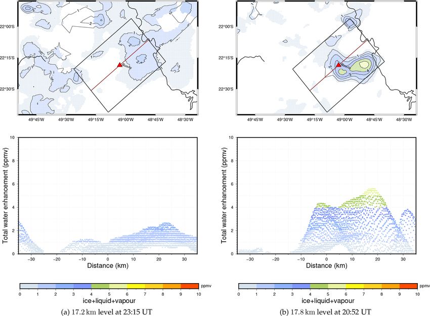
882                                                                               A. K. Behera et al.: Overshooting convection

1   Introduction                                                    et al. (2018) establishes that the hydration process takes over
                                                                    the dehydration process at the tropopause level from De-
Water vapour (WV) concentrations in the stratosphere im-            cember 2008 to February 2009. Schoeberl et al. (2018) also
pact both chemistry (Shindell et al., 1999; Shindell, 2001;         shows a 2 % increase in global stratospheric WV in a numer-
Herman et al., 2002) and Earth’s radiative balance (Forster         ical model by just introducing deep convection. Nonetheless,
and Shine, 2002). It also contributes to the formation of po-       at a large or global scale, the relative contribution of strato-
lar stratospheric clouds (Toon et al., 1990; Hervig et al.,         spheric overshoots to the cold trap remains unknown (Smith,
1997). WV is the primary greenhouse gas on Earth (Rind,             2021).
1998), essentially in the upper troposphere and lower strato-          In recent years, studies suggest that deep convection reach-
sphere (UTLS), aside from its chemical effects. Furthermore,        ing the tropopause may influence the stratospheric WV bud-
Solomon et al. (2010) discusses the non-negligible fluctua-         get on a large scale. Subsequently, the deep convection is now
tions in surface temperatures caused by minute changes in           a part of trajectory domain-filling studies of stratospheric
stratospheric WV over a decadal timescale.                          WV distribution (e.g. Schoeberl and Dessler, 2011; Wright
   The tropical tropopause layer serves as a gate where water       et al., 2011; Ueyama et al., 2015). Schoeberl et al. (2012)
enters the stratosphere (Brewer, 1949; Holton et al., 1995).        cannot rigorously conclude on the quantitative characterisa-
In the first order, the very cold temperature field across the      tion of convective moistening of the stratosphere because of
tropical tropopause layer (TTL) constrains the abundance of         its small contribution. Furthermore, it is below the precision
WV in the stratosphere (Holton and Gettelman, 2001; Ran-            level of satellite H2 O measurements. Nonetheless, Schoeberl
del et al., 2001). The TTL is a transition zone around the          et al. (2012) parameterise the impact of deep convection pro-
tropical tropopause extending from 14 to 19 km with inter-          ducing gravity waves to mitigate the TTL hydration. Ueyama
mediate properties between the troposphere and the strato-          et al. (2015) estimate an enhancement of ∼ 0.3 ppmv of H2 O
sphere (Folkins et al., 1999; Fueglistaler et al., 2009). Inside,   across 100 hPa at a large scale in the Southern Hemisphere
above the level of zero radiative heating, air masses progres-      during the austral summer of 2006–2007 from a trajectory-
sively ascend and get dehydrated due to solid condensation or       based study; the trajectories are initialised from the satellite-
sedimentation of ice particles, a process known as the cold-        observed convective cloud tops. Advancing further, Ueyama
trap mechanism (Sherwood and Dessler, 2000). The first tra-         et al. (2018) report an enhancement of about 0.6 ppmv WV
jectory studies by Fueglistaler et al. (2005) and James et al.      at this level between 10◦ S and 50◦ N during the 2007 boreal
(2008), which ignored the contribution of deep convection in        summer. Carminati et al. (2014) obtain an indirect signature
the TTL, show agreement with the abundance and variability          of the stratospheric overshoots at a global scale by studying
of WV in the tropical tropopause as measured by satellite-          the diurnal cycle of the EOS Aura MLS (Microwave Limb
borne sensors, confirming the cold trap as the principal mech-      Sounder) H2 O mixing ratio due to deep convection over-
anism dominating WV entry into the tropics. Nonetheless,            shooting the 100 hPa layer, highlighting the most active con-
open-ended debates over the trend of stratospheric WV (Olt-         vective regions. However, the critical impact of stratospheric
mans et al., 2000; Rosenlof et al., 2001; Randel et al., 2006;      overshoots on the global distribution of WV has so far proven
Scherer et al., 2008) and tropopause temperature (Seidel and        difficult to estimate.
Randel, 2006) in the 1990s and 2000s demonstrate that addi-            Another potential strategy is to upscale stratospheric over-
tional factors may be at play in the processes that determine       shooting effects by forcing them into a large-scale simula-
WV entering the stratosphere (Randel and Jensen, 2013).             tion, where the overshoots are explicitly resolved in cloud-
   One identified factor is the deep convection in the tropics,     resolving numerical simulations. However, cloud-resolving
overshooting the stratosphere. It injects ice particles directly    simulation studies of several cases must be conducted be-
above the tropopause, which may experience partial sublima-         fore proceeding with this phase. The combined study of
tion before falling back to the troposphere. Consequently, the      results corroborated by observations would encourage a
net effect should be hydration that mitigates the large-scale       stratospheric overshoot nudging strategy in a larger-scale or
dehydration effect. Recently many case studies, based both          Brazilian size simulation. Furthermore, utilising the superpa-
on modelling (e.g. Chaboureau et al., 2007; Grosvenor et al.,       rameterisation method (Grabowski, 2001; Khairoutdinov and
2007; Chemel et al., 2009; Liu et al., 2010; Dauhut et al.,         Randall, 2001; Khairoutdinov et al., 2005), explicitly adding
2015) and observations (e.g. Corti et al., 2008; Khaykin et al.,    a cloud-resolving simulation in each grid or subgrid point of
2009; Iwasaki et al., 2012; Sargent et al., 2014; Khaykin           a general circulation model (GCM) simulation or sub-GCM
et al., 2016; Jensen et al., 2020), have validated the hydration    simulation to consolidate the local-scale aspects such as the
effect of stratospheric overshoots at local scales in the trop-     diurnal cycle and convection strength (e.g. Khairoutdinov
ical belt. Occasionally, studies have shown that if the lower       and Randall, 2006; Randall et al., 2016), would provide in-
stratosphere is saturated with ice, the net effect is dehydra-      formation on the influence of overshoots at a large scale. The
tion by ice crystal growth in the stratosphere, removing WV         goal of this research is to learn more about cloud-resolving
by sedimentation (Hassim and Lane, 2010; Danielsen, 1982).          simulations.
The forward domain-filling trajectory model by Schoeberl

Atmos. Chem. Phys., 22, 881–901, 2022                                                  https://doi.org/10.5194/acp-22-881-2022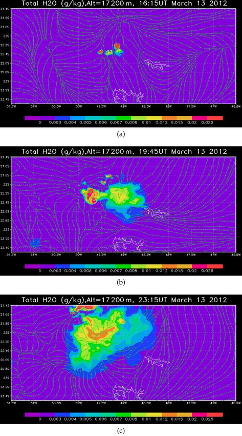
A. K. Behera et al.: Overshooting convection                                                                                  883

   Here, we perform three simulations of an observed case          with volumes of 500 and 1500 m3 , as well as 1.2 kg To-
of stratospheric overshoots using the BRAMS (Brazilian ver-        tex rubber balloons that were somewhat larger than conven-
sion of the Regional Atmospheric Modeling System; RAMS)            tional radiosonde balloons, were used. The TRO-Pico cam-
mesoscale model. They are different from each other in terms       paign provided measurements of CO2 , CH4 , O3 , and NO2
of the microphysical setup or the vertical grid structure. As      using a large set of equipment. On the other hand, WV
a result, this study generates a variety of estimations for        and particle measurements were the campaign’s main sam-
ice injection into the stratosphere and water remaining af-        pling. Only the Pico-SDLA and FLASH-B WV-measuring
ter sublimation. We use the data from a well-documented            devices, along with the light optical aerosol counter (LOAC)
case on 13 March 2012 in Bauru, São Paulo state, Brazil,           and COBALD particle measurement equipment, were flown
during the TRO-Pico, a small balloon campaign (Khaykin             on 13 March 2012. The balloons collected data with a ver-
et al., 2016; Ghysels et al., 2016). On that particular day,       tical resolution of approximately 20 m. Readers interested
two lightweight balloon-borne hygrometers intercepted a hy-        in balloon-borne measurement technology may read Vernier
drated stratospheric air parcel emanating from two distinct        et al. (2018) and Pommereau et al. (2011), as well as the ref-
overshooting plumes. However, no ice particles were de-            erences in those papers, which are based on large balloon
tected by the particle counter and backscatter sondes. It is       campaigns, BATAL and HIBISCUS, respectively.
also worth noting that at these altitudes, the relative humidity      Pico-SDLA is an infrared laser hygrometer emitting at
with respect to ice was reported to be about 40 %–50 %.            2.61 µm in a 1 m long open optical cell (Ghysels et al., 2016).
   The paper is organised as follows: Sect. 2 gives a concise      Its uncertainty is about 4 % in the TTL conditions. FLASH-B
description of the observed case, as well as the TRO-Pico          is a Lyman-α hygrometer measuring WV at nighttime only
campaign and the balloon-borne devices utilised for WV             with an uncertainty of 5 % in the UTLS (Khaykin et al.,
measurements. The BRAMS model and the setup of the three           2009). LOAC is an optical particle counter based on the scat-
simulations are described in Sect. 3. The TRO-Pico observed        tered light at 60◦ by ambient aerosol or particles for different
dataset is used to validate the simulations in Sect. 4. The key    wavelength channels (Renard et al., 2016). COBALD, de-
findings are discussed in Sect. 5, which depicts the structure     veloped at ETH Zürich, is a backscatter sonde that applies
and composition of overshooting plumes. The stratospheric          several wavelengths (Brabec et al., 2012). Here, we use both
WV mass budget is studied quantitatively in Sect. 6. Finally,      the particle/aerosol instruments for the ice particle detection
Sect. 7 summarises the work’s primary findings as well as          above the tropopause level.
upscaling strategies.
                                                                   2.2   Meteorological conditions, flight trains, and
2     Observational case of 13 March 2012 at Bauru                       balloon-borne measurements

2.1    Overview of TRO-Pico campaign
                                                                   Before discussing the details of the observations, we sum-
                                                                   marise the meteorological conditions on 13 March 2012, in
TRO-Pico is a French initiative based on a small bal-              the central region of the state of São Paulo. This day was
loon campaign in Bauru (22.36◦ S, 49.03◦ W), state of São          after the peak of the rainy season, with frequent heavy thun-
Paulo, Brazil, and funded by the Agence Nationale de               derstorms. There was no noticeable deep convective activ-
la Recherche (ANR). Its purpose is to study the strato-            ity around Bauru before local noon (15:00 UT). The syn-
spheric water vapour entry in the tropics at different spa-        optic situation during the entire day exhibited an extremely
tial and timescales. In particular, TRO-Pico’s main goal           weak pressure gradient across all of São Paulo, with very
is to better quantify the role of overshooting convection          light westerly winds in the mid-levels of the troposphere.
at a local scale in order to better quantify its role at a         Nonetheless, a vigorous thermodynamic instability prevailed
larger scale with respect to other processes. It took place        throughout that afternoon. At IPMet in Bauru, convective
in March 2012 for the first intensive observation period           available potential energy (CAPE) values of 4000 J kg−1
(IOP) and from November 2012 to March 2013, with regu-             were forecast in the central and western parts of São Paulo
lar soundings including a second IOP in January and Febru-         state by the meso-ETA weather model (Mesinger et al., 2012;
ary 2013. The case under investigation in this paper is part       Betts and Miller, 1986), of which an adapted version (Held
of the first IOP, while Behera et al. (2018) investigated          et al., 2007) was routinely running with a horizontal resolu-
the November 2012 to March 2013 TRO-Pico period. Sev-              tion of 10 km × 10 km during the TRO-Pico campaign. These
eral lightweight devices were used in this campaign, in-           conditions were indeed favourable for the development of
cluding Pico-spectromètres à diode laser accordables (Pico-        relatively small and short-lived deep convective cells, which
SDLA), which weighs 8 kg, the Fluorescent Advanced                 started to appear from local noon. The main convective ac-
Stratospheric Hygrometer for Balloon (FLASH-B), which              tivity in the area of interest for the TRO-Pico campaign was
weighs 1 kg, and compact optical backscatter aerosol de-           about 100 km east of Bauru near Botucatu, and later between
tector (COBALD), which weighs 1.3 kg. Hydrogen/helium-             Botucatu and Bauru with a series of short-lived and almost
inflated Raven Aerostar zero-pressure plastic (open) balloons      stationary convective cells. The reader is referred to Sect. 4

https://doi.org/10.5194/acp-22-881-2022                                              Atmos. Chem. Phys., 22, 881–901, 2022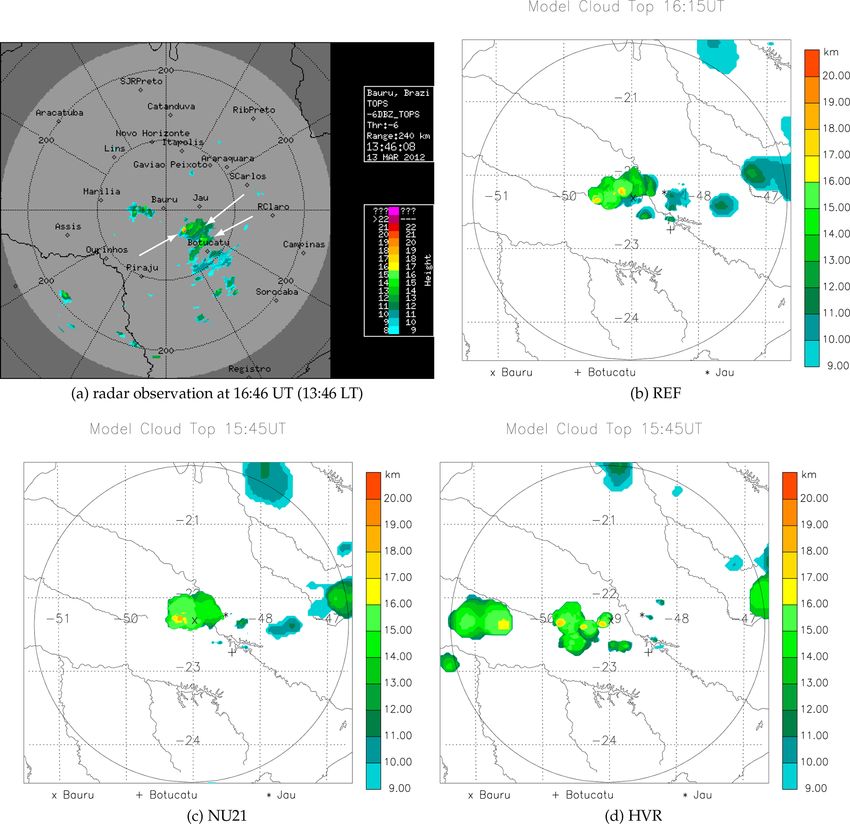
884                                                                               A. K. Behera et al.: Overshooting convection

and the animation on cloud tops in the Supplement for the           it may underestimate the altitude and size of the overshoot-
time evolution of the convective cells at these locations.          ing plumes containing small cloud droplets and mostly ice
   On 13 March 2012, a flight train comprising Pico-SDLA            particles when they are at a relatively long distance from the
and LOAC sensors was launched at 20:20 UT under a 500 m3            station.
Aerostar open balloon. The balloon reached the upper TTL
around 21:54 UT and began to descend at around 22:00 UT             3     BRAMS mesoscale model and simulation settings
under a parachute from ∼ 24 km altitude. A total of 3 h later,
after the launching of Pico-SDLA, another flight train com-         3.1    Brazilian developments on the Regional
prising FLASH-B and COBALD instruments was launched                        Atmospheric Modeling System (BRAMS)
under a 1.2 kg Totex extensible balloon. This balloon burst
at 23:39 UT. Ghysels et al. (2016) and Khaykin et al. (2016)        BRAMS, version 4.2, maintained at Centro de Previsão de
report on the WV profiles from both stratospheric hygrome-          Tempo e Estudos Climáticos (CPTEC) (Freitas et al., 2009),
ters. Within a layer from altitude 15 to 21.2 km, Ghysels et al.    is a 3-D regional and cloud-resolving model based on the
(2016) demonstrate a Pico-SDLA/FLASH Pearson correla-               RAMS model, version 5.04, developed at Colorado State
tion coefficient of 0.98, where both the hygrometers recorded       University (CSU)/ATMET (Cotton et al., 2003). The Brazil-
two particular local enhancements of the WV mixing ratio at         ian developments, tuned for the tropics, are essentially on
18.5 and 17.8 km altitude, respectively. Besides, they regis-       the cumulus convection, surface scheme, and surface mois-
tered a third local enhancement at 17.2 km altitude, albeit of      ture initialisation. It simulates the turbulence, subgrid-scale
smaller magnitude in comparison to the earlier two. One re-         convection, radiation, surface–air exchange, and cloud mi-
markable point is that the LOAC particle counter detected           crophysics with the two-moment configuration at different
no ice particles within these altitudes during the flight train.    scales ranging from large continental to large-eddy-scale
Moreover, the COBALD backscatter sonde flown under the              simulations. Additionally, it can simulate seven types of hy-
same balloon as FLASH ruled out the presence of ice parti-          drometeors, viz., cloud, and rain as liquid particles and pris-
cles.                                                               tine ice, snow, aggregate, hail, and graupel as ice particles
   The trajectory study of Khaykin et al. (2016) establishes        (Walko et al., 1995). Here, the mixing ratios of hydromete-
a well-documented link between the local enhancement of             ors and concentration are prognostic variables (Meyers et al.,
WV in the stratospheric part of the TTL, seen by Pico-SDLA          1997). A gamma distribution represents all hydrometeors,
and FLASH-B, and the air mass advected from stratospheric           where ν, the shape parameter, determines both the modal di-
overshooting plumes. However, based on a more extensive             ameter and the maximum concentration at that diameter.
investigation of a deep convective system that developed dur-
ing the local afternoon of 13 March 2012, in the southeast of                     1

                                                                                       D ν−1 1

                                                                                                     D

Bauru, and decayed in the evening, the current work provides        fgam (D) =                 exp −                           (1)
                                                                                 0(ν) Dn    Dn       Dn
additional insights into the time evolution of this meteorolog-
ical state. A comparison between Bauru S-band radar images             In Eq. (1), fgam denotes the probability density function
with model outputs is made in Sect. 4 to monitor the detected       for the modified gamma distribution of hydrometeors with a
convective activity and development of specific plumes.             diameter of D, as obtained from (Walko et al., 1995). 0(ν) is
                                                                    the normalisation constant, and Dn is the characteristic diam-
2.3   S-band radar
                                                                    eter of the modified gamma distribution. A bigger ν indicates
                                                                    a narrower distribution width and a larger modal diameter.
This modelling study benefits from the echo tops product of         As a result, the proportion of smaller and bigger hydromete-
convective systems observed by the Doppler S-band radar,            ors in the distribution is modulated. The size distribution of
located at IPMet/UNESP in Bauru. It facilitates the valida-         hydrometers would be more peaked as the modal diameter
tion of our simulations. The echo top measurements depend           increased.
highly on the technical specifications of the radar, such as           Furthermore, using a smart grid-nesting system that solves
wavelength, beam width, pulse width (PW), pulse repetition          equations simultaneously between computational meshes
frequency (PRF), and radial and azimuth resolution. In the          while applying any number of two-way interactions, the
case of Bauru S-band radar, the beam width is 2◦ ; the PW           BRAMS/RAMS can solve the fully compressible non-
is 0.8 µs at a PRF of 620/465 pulses per second, limiting           hydrostatic equations (Tripoli and Cotton, 1982). It also in-
the range to 240 km with a radial resolution of 250 m and           cludes a deep and shallow cumulus system based on the Grell
1◦ in azimuth. Thus, the Bauru radar can only identify rain-        and Dévényi (2002) mass flow approach, which can be used
drops, liquid, or frozen particles, with a general threshold of     to simulate tracer convection. Marécal et al. (2007) are able
10 dBZ, corresponding to a rainfall rate of 0.15–0.3 mm h−1         to simulate the WV distribution in the tropical UTLS in a
when the beam cross section is filled. The radar records re-        deep convective atmosphere using this model. Similarly, Liu
flectivity, spectral width, and radial velocities at 16 different   et al. (2010) simulate stratospheric overshooting convection
elevations between 0.3 and 45◦ . Due to the 2◦ beam width,          and concomitant WV increases in west Africa during the

Atmos. Chem. Phys., 22, 881–901, 2022                                                 https://doi.org/10.5194/acp-22-881-2022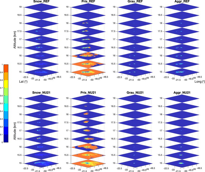
A. K. Behera et al.: Overshooting convection                                                                                   885

monsoon. The latter study was limited to balloon-borne WV          the state of São Paulo, centred at 22.4◦ S, 49.0◦ W, slightly
measurements from the African Monsoon Multidisciplinary            south of Bauru. The area of the third grid covers the most
Analysis (AMMA) campaign and brightness temperatures               active convective region around Bauru with a domain size
from the Meteosat Second Generation (MSG) satellite, re-           of 201 km × 165 km, centred at 22.1◦ S, 49.2◦ W. We restrict
sulting in limited quantitative data on overshoots. However,       the top layer of the domain to 30 km altitude with a sponge
S-band radars are used in the current investigation to better      layer of 5 km to absorb gravity waves at the top on a terrain-
constrain deep convective cells both spatially and temporally.     following σ -coordinate system, regardless of the vertical res-
                                                                   olution of the simulations.
3.2     Simulation setups
                                                                      Each simulation begins at 12:00 UT on 12 March 2012,
                                                                   and ends 48 h later. To reduce computing costs, we activated
We use the BRAMS model to run three cloud-resolving sim-           the third grid only at 10:00 UT on 13 March and recorded
ulations, including multiple grid-nesting to explicitly address    model outputs every 7.5 min after that. This data record fre-
the stratospheric overshoots associated with the case study in     quency corresponds to the volume scans produced by the IP-
Sect. 2. In these simulations, the modelling strategy is to as-    Met S-band radar. These are used to validate the cloud-top
sess the sensitivity of the stratospheric water budget linked      models. To ensure numerical stability, the simulation integra-
to overshoots to the model setup, such as microphysical pa-        tion time step varies between 2 and 10 s for the coarsest grid.
rameters or vertical resolution, resulting in various hydration    It is 5 times smaller for the second grid and 25 times lower
or ice injection amounts. It is likely to have an impact on our    for the third grid. Invoking the radiation module has a time
conclusions about the underlying physical characteristics re-      resolution of 300–500 s. The ECMWF operational analyses
lated with overshoots, as well as the mechanism for setting        with 1.0◦ spatial resolution initialise all simulations and force
them up in large-scale H2 O nudging scheme simulations (or         the first grid’s boundary conditions every 6 h. Following the
Brazilian size). We employ the same domain (mother grid)           work of Liu et al. (2010), there is no nudging of ECMWF
as a step forward from Behera et al. (2018) seasonal-scale         data at the domain’s centre.
study, where the model cannot explicitly resolve the over-
shoots. Then we raise the spatial resolution until we reach
                                                                   3.2.2   Specific setup
the third grid, ensuring that the overshoots are explicitly re-
solved. We start the simulation several hours before the onset     REF, NU21, and HVR simulations deviate from each other
of deep convection activity in the radar data, because we will     over the following points.
use Bauru radar observation to evaluate the development of
convective cells, as mentioned in Sect. 2.3, and to give the         – The shape parameter (ν) in the gamma function distri-
model enough time to spin up.                                          bution concerning the hydrometeors is ν = 2.0 in REF;
   Following that, we run three simulations with a spatial res-        however, it is ν = 2.1 in NU21. On 13 March 2012,
olution of 800 m × 800 m. The first of the three simulations           at 10:00 UT, we introduce this setting to all the grids
is the reference simulation (REF). The shape parameter (ν)             of NU21. Both NU21 and REF are exactly equal un-
of the hydrometeors in the bulk microphysics setting differs           til this point in time. The goal here is to investigate the
from REF in the second simulation, which is indicated as               impact of this microphysical parameter, the size distri-
NU21 (ν = 2.1). NU21 is projected to produce hydromete-                bution of various hydrometeors, during the most active
ors with greater mean mass diameters. To better assess TTL             time of deep convection in order to avoid any potential
dynamics, the third simulation, denoted HVR (high vertical             early divergence. Note that Penide et al. (2010) perform
resolution) hereafter, has a greater vertical grid-point resolu-       a cloud-resolving scale simulation using the BRAMS
tion than REF and NU21. The impact of NU21’s sensitivity               model to explore the hydrometeors’ size distribution in
on the microphysical component, as well as HVR’s vertical              mesoscale convective systems applying ν = 2.0.
resolution, on simulations of deep convection and overshoot-
ing plumes, is then examined.                                        – HVR differs from REF with respect to the vertical grid-
                                                                       point resolution in the TTL. REF has 68 vertical levels
3.2.1    General setup
                                                                       with about 300 m resolution within the TTL, whereas
                                                                       HVR has 99 vertical levels with typically 150 m verti-
REF, NU21, and HVR comprise the grid-nesting system of                 cal resolution within the TTL, except at the tropopause
three grids holding the same grid positions and the same               level where it is 100 m. Unlike REF and NU21, HVR
horizontal grid-point presentation. The horizontal grid-point          is carried out entirely at the higher vertical resolution
resolution increases from 20 km, parent grid, to 4 km in the           starting at 12:00 UT on 12 March 2012. In the BRAMS
second grid and 800 m in the third grid. The parent grid en-           model, it is unfeasible to change the vertical grid struc-
compasses a large part of southern Brazil with a domain of             ture in the middle of the integration of simulation unless
1840 km × 1640 km, centred at 23◦ S, 49.9◦ W. The second               each layer in REF would correspond to a layer in HVR,
grid comprises a domain of 964 km × 624 km, encompassing               which is not the case here.

https://doi.org/10.5194/acp-22-881-2022                                               Atmos. Chem. Phys., 22, 881–901, 2022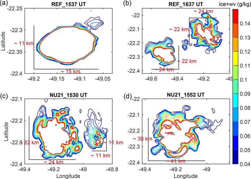
886                                                                             A. K. Behera et al.: Overshooting convection

4     Validation of the simulations                               complex to have developed at 16:15 UT west of Bauru, de-
                                                                  picting two cloud tops of height greater than 17 and 18 km,
We validate the three BRAMS simulations using observa-            respectively. At 15:45 UT, NU21 (Fig. 1c) indicates a similar
tions from the S-band radar of IPMet, located in Bauru, and       convective system in the west of Bauru, as seen on the radar
the balloon-borne measurements of the TRO-Pico campaign,          image (Fig. 1a) 1 h later in the southeast of Bauru, but with
respectively. Note that the balloon-borne measurements are        only one cloud top greater than 18 km level. HVR (Fig. 1d)
part of the first IOP phase of the 2-year field campaign.         also produces a convective cluster at 15:45 UT in the west
                                                                  of Bauru but comprising three cells in the vicinity of Bauru,
4.1    Validation of modelled cloud tops against radar            100 km, with two cloud tops of height greater than 17 km and
       echo top observations                                      one greater than 18 km.
                                                                     The full time series of the comparison between the mod-
We examine the BRAMS model’s capacity to initiate and de-         elled cloud tops and the S-band radar echo tops is in the Sup-
scribe deep convection activity at an accurate time and loca-     plement (animation of cloud tops) every 7.5 min from 15:01
tion by comparing simulated outputs to S-band radar data. To      to 18:52 UT on 13 March 2012. Figure 1 demonstrates the
do so, we estimate the modelled cloud-top layers every 1 km       main features of this series of comparison at the peak of
at altitudes ranging from 9 to 20 km, much like the echo top      the convective activity. The radar is largely cloud free at the
products. We determine the modelled cloud-top height for          start of the convective activity (15:01 UT); the only convec-
this altitude range if the concentration of condensed water,      tive cells are around 100 km south–southeast of Bauru near
i.e. ice plus liquid, exceeds a specified mixing ratio thresh-    Botucatu, with tops typically at 9 to 10 km in altitude. REF
old within a specific layer. The cloud-top altitude assignment    reproduces this feature qualitatively with the same range of
for a given (x, y) grid mesh is conclusive once all the ver-      maximum height but much closer to Bauru, however, south–
tical levels are read because this criterion is implemented in    northwest of Bauru. The same type of storm cluster is ob-
a bottom–top loop. We use a threshold of condensed water          served in NU21 at 14:15 UT. About 45 min later, at 15:00 UT,
concentration to a cloud top based on its range of altitudes      NU21 produces convective activity triggering at the same po-
to account for the drop in hydrometeor concentration with         sition as in REF but with more intensity and higher cloud
altitude inside the TTL linked to a deep convective cell. It      tops. It highlights that deep convection triggers earlier in
is 1 g kg−1 for the layers ranging from 9–10 to 15–16 km. It      NU21. At 14:15 UT, there is no sign of convective activities
is 0.45 g kg−1 for 16–17 km, 0.2 g kg−1 for 17–18 km, and         in HVR, unlike in the radar image, but it appears at 15:00 UT
0.008 g kg−1 for layers above 18 km. These thresholds are         near Ourinhos – southwest of Bauru. The convective cells
chosen as a function of typical hydrometeor concentrations        are overgrown in the area than in NU21 at 14:15 UT, though
within overshooting plumes (see Liu et al., 2010).                in a similar position. By 15:00 UT, the deep convection alti-
   Figure 1 allows a qualitative comparison of the radar echo     tude in HVR is also higher than in REF and the radar echo
tops and modelled cloud tops from the three simulations. It       tops. It is also located much more west than the radar obser-
illustrates the capacity of BRAMS to reproduce the prin-          vations. However, stratospheric overshoots are present in the
cipal features: triggering deep convection, structure evolu-      simulations as well as in the radar observations with the echo
tion, and severity of the overshooting plume in this relatively   top above 17 km at the peak of the convective activity, i.e.
unorganised convective cluster. Note that here we compare         during 16:00–17:00 UT. In the three simulations, convective
the convective plumes when they are within a 100 km ra-           activity increases in height and spreads over larger areas in
dius of Bauru (the inner circle in Fig. 1a) to avoid a rela-      the TTL as time passes. In HVR, it is further west–southwest
tively large scanning angle of the radar and thus to obtain       of Bauru. Thus, all simulations predict the onset of convec-
accurate echo top heights. Furthermore and importantly, the       tive activity to be slightly earlier than observed. Given the
modelled cloud tops are well within the third grid, not near      uncertainties in modelling and S-band radar perceptions of
or at the edges of this grid. We observe that the model can re-   deep convective activity, associating one-by-one simulations
produce relatively well these highly unpredictable convective     with radar convective cells in spatial and temporal terms is
systems. There exist similar deep convective clusters around      a difficult task (e.g. Li et al., 2008; Rowe and Houze, 2014;
Bauru in the radar images and the simulations, although           Weisman et al., 1997). As a result, it may not be the most
at slightly different times. The radar image at 16:46 UT          appropriate criterion for evaluating these disorganised deep
(13:46 local time; Fig. 1a) shows a storm cluster comprising      convective cloud simulations.
three cells near Botucatu, southeast of Bauru with the echo          However, during the period 15:00–18:30 UT on
top of the furthest west one reaching higher than 18 km level.    13 March 2012, within a 100 km radius of Bauru, we
We should emphasise that small cloud droplets and ice par-        tabulate (Table 1) the number of overshooting plumes higher
ticles, which are the principal components of overshooting        than 17 km altitude – the radar threshold for detecting
plumes, are considerably less sensitive to the S-band radar       overshoots. It is to have a general understanding and knowl-
because they do not sufficiently fill the beam cross section.     edge with in the three cloud-resolving simulations. The
In REF (Fig. 1b), we notice a comparable convective storm         observation period is limited to 18:30 UT since the radar

Atmos. Chem. Phys., 22, 881–901, 2022                                               https://doi.org/10.5194/acp-22-881-2022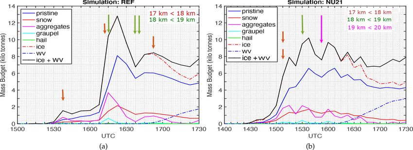
A. K. Behera et al.: Overshooting convection                                                                                            887

Figure 1. Snapshots of echo tops, observed by the S-band radar and modelled cloud tops from the BRAMS simulations on 13 March 2012,
centred at Bauru. (a) Radar observation at 16:45 UT, then (b–d) REF at 16:15 UT, NU21 at 15:45 UT, and HVR at 15:45 UT. The circle
displayed in panels (b), (c), and (d) corresponds to the 240 km radar range in (a). The arrows represent the three deep convective cells that
surround Botucatu, one of which has a cloud-top height greater than 18 km.

images reveal deep convection decaying after that time.                  rarely reach 19 km (see the animation on cloud tops in the
REF can produce an equal amount of overshooting plumes                   Supplement). HVR, on the other hand, has approximately 18
observed by the S-band radar, though at somewhat higher                  overshooting plumes during the observation period, which is
altitudes, as shown in Table 1. We expect this because radar             significantly more than REF (10 overshoots) and NU21 (6
sensitivity to low-ice content is low, causing the radar to              overshoots).
underestimate the number of overshoots. Furthermore, a                      To further understand the situation, one can expect HVR
situation in which the 380 K layer is below the 17 km altitude           to determine more reliable dynamics across the tropical
threshold is a reasonable explanation. The overall number                tropopause than REF and NU21, respectively. Contrary to
of overshooting cells in NU21, on the other hand, implies                expectations, it tends to intensify massive deep convec-
that it is less favourable than REF and radar at producing               tion activity. A plausible fact to explain such behaviour
overshooting plumes. The time series analysis of cloud                   in HVR is the ratio between vertical and horizontal grid
clusters indicates that the lifetime of overshooting plumes              points, which overestimates vertical motions due to grid
appears to be longer than REF, where overshooting plumes                 cell saturation (Homeyer et al., 2014; Homeyer, 2015). It

https://doi.org/10.5194/acp-22-881-2022                                                      Atmos. Chem. Phys., 22, 881–901, 2022
888                                                                                    A. K. Behera et al.: Overshooting convection

                                                                        might be the model’s Courant–Friedrichs–Levy (CFL) limit,
Table 1. Count of overshoots above 17 km altitude for the S-band        which in finite-difference simulation techniques constrains
radar (end time UT of the volume scan) and for the REF, NU21, and       the relationship between infinitesimal increases in space grid
HVR simulations. Their counts are represented as multiples of ×.        points and infinitesimal time step increments. In the BRAMS
Within a 1 km thick layer, the altitude is the lowest point. The mod-
                                                                        model, the von Neumann stability assessment (Deriaz and
elled overshoots are calculated by taking into account the height
                                                                        Haldenwang, 2020) is necessary for the transport equations
of each plume in the 7.5 min time-lapse imagery, which must be
greater than or equal to 17 km, as well as the spatial spread of each   related to convection. Aside from that, Eulerian model sim-
plume. Figure 6 depicts a scenario in which the spatial extent of the   ulations of high vertical resolution, high-frequency wave
overshoot is also taken into account.                                   motions, such as inertia–gravity waves (e.g. Staquet, 2004;
                                                                        Young, 2021), can be overdetermined. As a result, they can
 End of 7.5 min           Altitude (±0.5 km) and number of plumes       exaggerate cloud microphysics (Aligo et al., 2009) and cause
 volume scan (UT)      Radar         REF        NU21         HVR        erroneous cloud conditions near the TTL (Jensen and Pfister,
                                                                        2004). Therefore, we leave HVR out of the next sections to
 15:08                                         17   2×
                                                                        describe the details, and we do not look at this simulation’s
 15:15                                                                  water budget in the lower stratosphere.
 15:22                                                     17   1×         In Sect. 4.1, we essentially outline several principal as-
                                                                        pects by closely studying the simulated convective plumes.
 15:29                                         18   1×
                                                                        First, we locate the position of deep convective activity fur-
 15:37                             17   1×                              ther west–northwest in the model, typically 50 to 60 km
                                                           17   2×      west–northwest. Second, the time evolution of the convec-
 15:46
                                                           18   1×      tive clusters reveals that they are moving north–northwest,
 15:53                                         19   1×                  while most of the convective activity remains in the west of
                                                                        the Tietê River in both cases. Overall, we cannot expect the
 16:01
                                                                        model to predict precisely the position and time of convec-
 16:08               18     1×                             19   2×      tive activity development. REF and, to a certain extent, NU21
                                   17   1×                              provide reasonable predictions in space and time. They gen-
 16:15
                                   18   1×                              erate good estimates of convective cloud tops but initiate the
 16:22               17     1×                             17   3×      plumes generally earlier compared to the radar observation.
                                                                        In contrast, HVR yields unfavourable conditions and exag-
 16:29
                                                                        gerates its size.
                                   18   2×                 17   1×
 16:37
                                                           18   1×
                                                                        4.2     Validation against TRO-Pico balloon-borne
 16:46               19     1×                             18   1×              measurements
                     18     1×     17   1×
 16:53                                                                  The WV and particle measurements performed in the vicin-
                     19     1×
                                                                        ity of overshoots in the frame of the TRO-Pico campaign es-
 17:01
                                                                        tablish a well-documented database to validate model sim-
 17:08               18     2×                                          ulations. For our study, as the balloon-borne measurements
 17:15                                                                  belong to a moment several hours after the overshooting
                                                                        event – this time interval between the overshooting event
 17:22               18     1×
                                                                        and the balloon-borne measurements is indicated as δtom
 17:29                                                     18   2×      hereafter; the simulation validation strategy is as follows.
 17:37               19     1×     17   1×                 18   1×      We observe the modelled overshooting plume at 17.2 and
                                                                        17.8 km altitudes, respectively, where FLASH-B and Pico-
 17:46                                         17   1×
                                                                        SDLA hygrometers captured the WV local enhancements
 17:53                             17   1×                              (see Khaykin et al., 2016). Then, after the same δtom , we in-
 18:01                                                     17   1×      vestigate the WV enhancement at these levels in the model.
 18:08                             17   1×
 18:15                                                                  4.2.1    REF simulation

 18:22                                                     17   2×      To validate the local WV enhancement at 17.2 km altitude
 18:29                             17   1×                              due to the modelled overshoots, we combine the TRO-Pico
                                                                        measurements by FLASH-B at 23:45 UT corresponding to an
 18:37                                         17   1×
                                                                        overshooting event that occurred at 16:46 UT with δtom = 7 h
                                                                        on 13 March 2012. We observe the time evolution of the

Atmos. Chem. Phys., 22, 881–901, 2022                                                      https://doi.org/10.5194/acp-22-881-2022
A. K. Behera et al.: Overshooting convection 889
Figure 2a illustrates REF determined overshooting plume
at 22.2◦ S, 49.15◦ W, entering the stratosphere at 16:15 UT.
About after 3.5 h, we observe this plume spreading wide hor-
izontally (Fig. 2b), mostly east to 49.4◦ W. Furthermore, sev-
eral other overshooting plumes developed in between but did
not interact with the eastern part of the convective plume.
Around 23:15 UT (Fig. 2c), most of the original plume
moved eastward of 49.1◦ W by advecting northward, as pre-
cisely as described in the trajectory analysis of the same case
in Khaykin et al. (2016). At some positions within the over-
shooting plume corresponding to the maxima of H2 O mix-
ing ratio (ice, liquid, and vapour), we obtain the local en-
hancement is typically 2 ppmv of the total water content (see
Fig. 3a) at this altitude within ±35 km northeast of Bauru.
Figure 3 highlights such H2 O enhancement domains in
isolines. In Fig. 3a, at 23:15 UT around Bauru within an area
of 70 km × 50 km, tilting northeast following the analysis in
Fig. 2, REF produces many grid points representing H2 O
enhancement of about 0.5 ppmv at 17.2 km altitude, which
is in agreement with FLASH-B and Pico-SDLA measure-
ments. The confirmation of no ice remaining indicates that
all the ice has sublimated or sedimented in the simulation. It
agrees with the measurements carried out using LOAC and
COBALD under the Pico-SDLA and FLASH-B, where they
did not detect any ice particles in the stratosphere. The mod-
elled 0.5 ppmv enhancement at the 17.2 km level is compa-
rable to the one measured by FLASH-B, 0.45 ppmv, in that
range of altitude. REF also produces very high H2 O enhance-
ment, greater than 10 ppmv, in the northwest region away
from Bauru. Such extremely wet conditions are possible due
to a very recent overshoot in this area in the simulation.
Then, we implement the same strategy to validate the hy-
dration due to overshoot at 17.8 km altitude; see Fig. 3b. It
is the altitude of the second water enhancement captured by
both Pico-SDLA and FLASH-B hygrometers. Khaykin et al.
(2016) report this H2 O enhancement comes from another
overshooting plume than the one explaining the 17.2 km
Figure 2. BRAMS simulation: REF total water content, ice, liq- H2 O enhancement. We investigate if a realistic overshoot-
uid, and vapour in g kg−1 , at 17.2 km altitude at (a) 16:15 UT, ing plume in BRAMS can appear with a similar H2 O en-
(b) 19:45 UT, and (c) 23:15 UT, respectively. The streamlines rep- hancement following the same δtom time around Bauru. For
resent the horizontal wind fields within the domain, a composite of the H2 O enhancement at 17.8 km altitude identified by Pico-
the second and third grids. SDLA at 22:04 UT, the associated overshooting event oc-
curred at 17:38 UT. This implies the δtom = 4 h 26 min. Fol-
lowing the overshooting plume, as in Fig. 2, from 16:15–
modelled (REF) overshooting plume at 17.2 km altitude from 20:52 UT, REF yields a similar δtom while obtaining the H2 O
16:15 UT to 23:15 UT to maintain the same δtom . Figure 2 enhancement. REF produces many grid points/pixels with
illustrates the horizontal cross section of the total water con- H2 O enhancement of 0.7 ppmv around Bauru within an area
tent at 17.2 km altitude at three different time stamps, viz., of 70 km × 50 km. Some pixels show more than 2 ppmv of
16:15, 19:45, and 23:15 UT, sequentially. It also draws the H2 O enhancement. Here, it is notable that BRAMS computes
horizontal wind streamline to follow the direction of the no ice in this part of the plume, which is in agreement with
moving plume at this height. We prepare this kind of plot the COBALD and LOAC measurements. The 0.7 ppmv lo-
every 7.5 min to follow the evolution of the overshooting cell cal enhancement at 17.8 km is thus fully compatible with the
at that height. For simplicity and due to space limitations, we one measured by Pico-SDLA, 0.65 ppmv, and by FLASH-B,
show only these three plots in the paper. 0.55 ppmv, at this altitude.
https://doi.org/10.5194/acp-22-881-2022 Atmos. Chem. Phys., 22, 881–901, 2022890 A. K. Behera et al.: Overshooting convection
Figure 3. REF providing total water (ice, liquid, and vapour) enhancement at (a) 17.2 km altitude at 23:15 UT and (b) 17.8 km altitude at
20:52 UT, respectively. The top panel shows the horizontal cross sections of the vertical grid at these altitudes, depicting the only grid points
when their total water content is higher than the model levels simply above and below in a vertical column. The isolines show the enhanced
total water content (ppmv) with respect to the model layer below it. The bottom panel shows the grid points’/pixels’ water content confined
by the northeast-tilting rectangle having the length of 70 km and half width of 25 km. The red triangle denotes Bauru (0 km); the northeast
direction is positive, and vice versa.
The purpose of the investigation is to witness the same where most of the original plume is north of 22.4◦ S and east
order H2 O enhancement in the model corresponding to the of 48.8◦ W at 23:15 UT.
TRO-Pico campaign measurements. And the approach of se- In Fig. 4a, the conclusions are similar to REF. The to-
lecting an area of 70 km × 50 km tilting in the northeast di- tal water content at 17.2 km altitude at 23:15 UT shows an
rection around Bauru is to consider only the H2 O enhance- enhancement of several ppmv, up to 2 ppmv at certain po-
ment within this area (see Fig. 3). Furthermore, it corre- sitions, particularly at the core of the plume. Many pixels
sponds to the point that the overshooting cells at 17.2 and within 10 km neighbourhood of Bauru show the WV en-
17.8 km heights, respectively, are induced by two separate hancement of half a ppmv near the border of the overshoot-
overshooting plumes (Khaykin et al., 2016). ing plume. It is compatible with the local enhancement mea-
sured by FLASH-B at 17.2 km height. Moreover, it is cru-
cial to recall the evidence of no ice remaining at this level,
4.2.2 NU21 simulation and the total H2 O is only in the vapour phase as observed
by the LOAC particle counter and the COBALD backscat-
With the same validation approach, as in REF, we select
ter sonde. Then, we analyse the WV enhancement in NU21
the overshooting plume that occurred at 16:15 UT in NU21.
at 17.8 km altitude at 20:52 UT, that is δtom = 4 h 40 min af-
We study the time evolution of the overshooting plume at
ter the 16:15 UT overshooting event (see Fig. 4b). This δtom
17.2 km altitude from 16:15 UT to (16:15 + δtom ) UT, that is,
is the same as the time interval between the Pico-SDLA
23:15 UT – δtom is 7 h from the overshooting event until the
measurement and the overshooting event. In Fig. 4b, we ob-
FLASH-B measurement. It is similar to that in Fig. 2 and
tain many pixels, located at the border of the overshooting
is provided in the Supplement (Fig. S1). The plume spreads
plume, with a ∼ 0.7 ppmv H2 O enhancement without any
horizontally, slightly southeastward, and finally northward,
Atmos. Chem. Phys., 22, 881–901, 2022 https://doi.org/10.5194/acp-22-881-2022A. K. Behera et al.: Overshooting convection 891
Figure 4. Like Fig. 3 but representing NU21.
ice remaining – a very similar way of observation to that by tive cloud tops are sometimes higher in altitude than the
Pico-SDLA and LOAC. Furthermore, there are many pixels radar images. It corresponds to a possible fact that the S-
near the Tietê River giving very high WV enhancement, up band radar is a little sensitive to the ice hydrometeors – the
to 6 ppmv. This sort of large water enhancement from over- main component of overshooting plumes addressed in sub-
shoots has already been identified by the FISH hygrome- sequent sections. The number of overshooting plumes above
ter aboard the Russian M-55 Geophysica high-altitude air- 17 km is comparable both in the model and the S-band radar
craft in the SCOUT-AMMA field campaign in west Africa images until 18:30 UT, after which the model exhibits con-
(see Schiller et al., 2009). It is now reasonable to state that vective activity with a longer lifetime. The study of over-
BRAMS simulated overshooting plumes responsible for the shooting plumes at 17.2 and 17.8 km altitude, respectively,
local WV enhancements; however, these were not necessar- and the corresponding total water enhancements after ∼ 4.5
ily exactly in the same locations as the observed ones. More- and 7 h, respectively, agree with both the balloon-borne mea-
over, the wind spreading about the overshooting plumes is surements of H2 O mixing ratio by Pico-SDLA and FLASH-
somewhat different from that in the realised ones during the B hygrometers. Moreover, note that the grid points showing
TRO-Pico field campaign. several ppmv of total H2 O enhancement are often at the edge
of the overshooting turret – coherent with the trajectory anal-
ysis of Khaykin et al. (2016), reporting that the air masses
4.3 Conclusion of the validation
sampled by the balloons are at the edge of the plume coming
In Sect. 4.2, we demonstrate that the BRAMS model, via from the overshoot.
REF and NU21, can simulate fairly realistic deep convec- Thus, this study brings to the fore that fine-scale simu-
tive plumes that are compatible with the IPMet S-band radar lations using the BRAMS model can reproduce the over-
observation during the temporal evolution of deep convec- shooting convection. Both REF and NU21 can lead now to
tive cloud systems over three hours. However, these mod- more insight into the overshooting plumes within unorgan-
elled deep convective plumes slightly west–northwest of the ised deep convective plumes. Certain standard features like
radar observation but with an intensity comparable to the de- the amount of ice injection, width and surface area of the
tected ones by the S-band radar. Furthermore, the convec- plume, H2 O mass flux, and the lifetime of the active cell,
https://doi.org/10.5194/acp-22-881-2022 Atmos. Chem. Phys., 22, 881–901, 2022892 A. K. Behera et al.: Overshooting convection
which we cannot directly measure with the current available thunderstorm and find (pristine) ice and snow as the pri-
resources, both REF and NU21, can now provide more in- mary components. However, the current study makes use of
sight into overshooting plumes within unorganized deep con- the BRAMS model, which combines five types of ice hy-
vective plumes. In the subsequent sections, we give a quan- drometeors rather than three in the WRF version used by
titative interpretation of the overshooting plumes from REF Chemel et al. (2009). Within the overshooting plume, Fig. 5
and NU21. Unfortunately, HVR appears to produce exces- also reveals a large amount of aggregates and graupel at the
sively severe convective activity, making it unsuitable for fur- tropopause level, particularly for REF. It is worth noting that
ther analysis. pristine ice is completely absent towards the plume’s deep-
est core at the base (16.6 km height, ∼ 380 K). Snow, aggre-
5 Analyses of overshooting turret gates, and, to a lesser extent, graupel are the only hydrom-
eteors that survive. The major ice hydrometeors in NU21
We provide the five conceivable combinations of hydromete- are snow particles, which disperse across a small area with
ors inside an overshooting plume to document the quantita- a radius of around 5 km. The overshooting dome at the edge
tive information collected from the simulations on the struc- of the plume near the tropopause level in all three scenar-
tural characteristics of a typical overshooting plume. Its base ios is entirely formed of pristine ice. In both scenarios going
is at the 380 K isentropic level, which is the stratosphere’s up to 18 km, well into the stratospheric region of the TTL,
lowest layer. At the 380 K isentropic level, the instantaneous only pristine ice (70 %) and snow (30 %) are the principal
mass flux of individual hydrometeors is also estimated. Be- constituents of the overshooting dome. Graupel and aggre-
tween the 380 and 430 K isentropic levels, it comprises the gates are present in REF but not in NU21. This finding is in
estimation of total ice mass and the five types of ice particles. line with sensitivity tests conducted by manipulating micro-
Finally, a table provides the quantities that could lead to a physics in Chemel et al. (2009) and Wu et al. (2009), who
road map of a nudging scheme of the water vapour enhance- used the WRF model to investigate convective updrafts dur-
ment in the lower stratosphere due to overshoots in large- ing the monsoon over Darwin, Australia. Our model illus-
scale simulations, which could lead to the quantification of trates an overshooting plume’s overall particle distribution as
the influence of overshoots on a large scale. well as its thermodynamic structure, which is controlled by
particle size distribution and affects the convective updraft.
The contact area or spreading (km2 ) of the overshoot-
5.1 Structure and composition of overshoots
ing plume at the lowest layer of the stratosphere, i.e. the
We assess all the five types of ice hydrometeors during an 380 K isentropic level, is then determined. Figure 6 depicts
overshooting event. The series of plots in Fig. 5 represents the spreading of overshooting plumes at this level for REF
the horizontal cross section of the ratio of different ice hy- and NU21 at various time steps as shown in Table 1. The
drometeors over the net ice varying with altitude around the average surface area of the propagation of the overshooting
TTL in the vicinity of the overshooting event that occurred plume at 380 K level is about 450 km2 , according to Fig. 6. It
at 16:15 UT in REF (see Table 1). We present this calcula- is roughly the grid-point resolution of a large-scale simula-
tion from 15:00 to 18:52 UT for REF and NU21, which can tion (400 km2 ), where Behera et al. (2018) show that with
be found in the animation of horizontal cross sections in the such horizontal grid-point resolution, BRAMS cannot ex-
Supplement. plicitly produce overshoots, and illustrate the TTL dynam-
Above the tropopause, we find pristine ice and snow to ics and WV variability at a continental scale during a full
be the primary ice hydrometeors (∼ 16.6 km altitude). How- wet season. In a cloud-resolving-scale simulation, BRAMS
ever, aggregates and a trace amount of graupel are present. It generates overshoots that spread over 450 km2 in the area at
is only true for REF. The full time evolution of the horizontal 380 K level, expanding from the third grid to the mother grid
cross section can be found in the Supplement. The lack of to disclose the intensity of convection. Hence, it is a criti-
this in NU21 could be attributed to its microphysical config- cal point to consider when planning an overshoot nudging
uration, which allows larger hydrometers to be placed deeper scheme.
within the convective plumes, resulting in a lower convec- Furthermore, we compare the horizontal spreading be-
tive updraft and inability to reach the tropopause layer. This tween REF and NU21. In Fig. 6, the upper panel repre-
is evident in Table 2 and Sect. 6.1, where REF is shown to sents the surface areas of REF, which are of 11 km × 15 km
release approximately 10 % more ice with a relatively higher at 15:37 UT and 22 km × 24 km at 16:37 UT, respectively.
flux rate at 380 K isentrope than NU21. Furthermore, as ex- In the case of NU21, the lower panel, the surface areas
pected at this level, the presence of hail particles is negligi- are of 22 km × 24 km and 11 km × 11 km at 15:30 UT, and
ble, as shown in Fig. 5, which confirms the results of Home- 30 km × 41 km at 15:52 UT, respectively. The latter one with
yer and Kumjian (2015), obtained using S-band radar mea- the large surface area indicates that changes in the particle
surements of deep convective activity over the extratropics. size distribution, the shape parameter ν, may modulate the
It is consistent with the results reported in Chemel et al. spreading of overshooting convection while penetrating the
(2009). Using the WRF model, they investigate the Hector stratosphere. In the following sections, we estimate the mass
Atmos. Chem. Phys., 22, 881–901, 2022 https://doi.org/10.5194/acp-22-881-2022A. K. Behera et al.: Overshooting convection 893
Figure 5. Vertical distribution of horizontal cross section of hydrometeors, viz., snow, pristine ice, graupel, and aggregates, within the third
grid, spanning over 15–19 km altitude. It is for the ratio of four types of ice hydrometeors against the entire ice content from REF – upper
panel, and NU21 – lower panel, shown at 16:15 UT. Hail is not included because of its negligible values within the plume.
budget corresponding to UTLS, set as a preferred range of as the principal hydrometeors are pristine ice and aggregates
isentropic levels. and to a much lower amount of snow and graupel, where the
order of magnitude of the maximum mass-flux rate of snow
and graupel is about 4-fold smaller than the maximum of
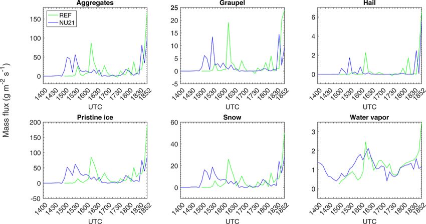
6 Stratospheric water mass budget
pristine ice and aggregates. Despite the non-negligible mass-
flux rate of graupel, its ratio in the structure of the overshoot-
We estimate each hydrometeor’s instantaneous mass-flux
ing turret remains modest. It occurs approximately 10 % of
rate across the 380 K isentropic level. The rates are the av-
the composition of overshooting plume in a limited area only
erage over the domain that comprises only the third grid of
in REF exceeding the tropopause level (∼ 16.6 km). Then,
simulation. Please note that it is not representative of a prop-
we associate the contrast in the snow composition inside the
erty of any particular overshooting plume but preferably ad-
plume with the sedimentation. Graupel, denser than snow,
dresses a realistic estimation on the flux rates of ice particles
falls faster to the troposphere, results in the accumulation of
entering the 380 K isentropic layer. Besides, we evaluate the
snow in the stratosphere. Though the overshoots begin at dif-
net H2 O mass budget prevailing within the slice of 380 to
ferent times in REF and NU21, the local maximum of mass-
430 K isentropic levels.
flux rates are of the same order of magnitude, and in REF, it
is regularly higher than NU21. It is already explicit that the
6.1 Mass flux across the 380 K isentropic level number of overshooting events is different in REF and NU21
(please refer to Table 1). Eventually, the differences in the
Figure 7 presents the domain-average instantaneous mass-
mass-flux rate between REF and NU21 would be critical to
flux rate for REF and NU21 across the 380 K isentropic level
explain as their values are also proportional to the vertical
over the third grid of the simulation during 14:00–18:52 UT.
wind velocity (see Sang et al., 2018).
It depicts primarily the inferences drawn from Fig. 5. Such
https://doi.org/10.5194/acp-22-881-2022 Atmos. Chem. Phys., 22, 881–901, 2022You can also read