Selkirk Golden Boy Project: Data Modelling and Interpretation

2015 University of Manitoba Geophysics Field School
              Selkirk Golden Boy Project: Data Modelling and Interpretation
                                     May 3, 2015

This information sheet is designed to guide you through analysis and modelling for the Selkirk Golden
Boy Project. You will start the modelling on a broad scale, with a series of exercises involving the whole
Golden Boy anomaly, and then you will work down to modelling the data collected this year. There are
also a series of questions designed to examine the sensitivity of the response to features at various
depths. The project will be written up as a technical report: the data collection and reduction already
completed and the modelling below will form the basis of the report. I recommend that you spend
about 3/4 of a day on the modelling and another 3/4 on the report. The modelling and the report can be
completed in pairs.

Regional Modelling

The aim of the large-scale geophysical modelling of the Selkirk potential field anomaly is to explain the observed
data in terms of major rock divisions. The modelling will not identify particular features such as ore bodies or
small-scale faults and folds.

Data from the original Golden Boy project are available at:
http://home.cc.umanitoba.ca/~frederik/Teaching/Field_School/Selkirk/Pro-Am_data/

1. Figure 1 shows a gravity and magnetic model for a profile running across the whole Selkirk anomaly
and 2-D modelling results. Approximately reproduce the results shown in this figure using POTENT.
Gravity data is available in the file 4-66com2.obs. For the gravity data, fit a profile running through the
short axis of the anomaly with a 2D polygonal prism. The prism should strike parallel to the long axis of
the anomaly. If you start with a prism of approximately the correct shape you can use a final inversion
step to adjust the locations of its apices so as to obtain the optimal fit to the data. Print both the body
and the fit to the data. The magnetic response is available in gbmag1.obs. Fit the data using several
small polygonal prisms. Comment on the density and susceptibility of the various bodies.

                                                        1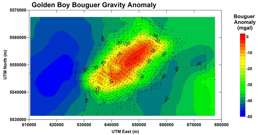

Figure 1. 2-D density and magnetic model of the Golden Boy anomaly (P. McGowan). Colour bodies are
density anomalies, black bodies are magnetic anomalies.

2. Use POTENT to obtain a 3D density model of the whole gravity anomaly (Figure 2). Remove the
regional trend and then use an ellipsoid, finite-length ellipsoidal cylinder, or dyke to fit the data. It is
not necessary to obtain a perfect fit to the data. Rather, we want to use the results to estimate overall
parameters such as the approximate volume of material with increased mass (assuming a density
contrast). Print both the body and the fit to the data and comment on the excess mass and volume of
the model.

                                                     2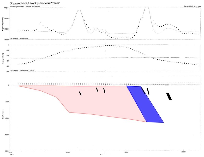

Figure 2. Golden Boy Bouguer gravity anomaly.

Preliminary Local Scale Modelling

The aim of the local-scale modelling is to examine the influence of possible smaller-scale structures on the
potential field response: will they be detectable?

3. (a) Use POTENT to examine the relative size and wavelength of gravity anomalies associated with:
realistic relief on the upper surface of the Phanerozoic and a moderate sized ore-body near the surface
of the Precambrian (10-20 million tonnes of ore). Comment on the results.
(b) Use POTENT to estimate the size of magnetic anomalies associated with a moderate-size ore body at
the top of the Precambrian.

Modelling Of PR67 and Adjacent Road Survey Results

The aim of this modelling is to explain the data obtained during the surveys conducted in the project.

4. Compare the Bouguer gravity anomaly for the PR67 profile with the results from the survey by Bill
Brisbin (Figure 3) which will be provided in the file PR67-airborne-brisbin.xls. You can subtract or
add a constant value to all points to bring the numbers to a suitable level for comparison.

5. Compare the results for the ground magnetic profiles with the aeromagnetic data (Figure 3) provided
in the file PR67-airborne-brisbin.xls. Comment on both the overall size of the anomaly and the spatial
wavelengths visible in the data.

                                                         3

Figure 3. ground gravity data and aeromagnetic data for profile along PR67.

6. Compare the short wavelength features on the ground profiles with the features shown on the
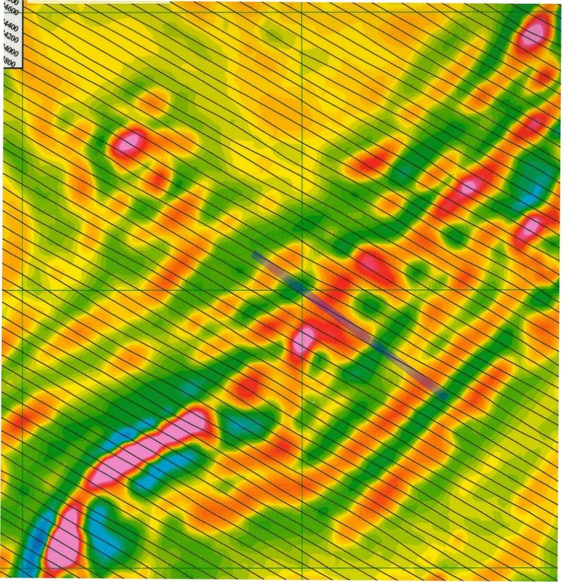
second vertical derivative map (Figure 4).

Figure 4. Second vertical derivative of total magnetic field showing approximate position of PR67 profile.
Grid lines are the 5000 m UTM grid.

                                                    4

7. Model the results of the PR67 magnetic survey using POTENT. Use as many geological, borehole,
and other constraints as possible. I suggest introducing a series of horizontal polygonal prisms of fixed
size, shape, and position, and varying the susceptibility of the prisms to obtain an optimal fit to the
data. The final adjustment of the susceptibilities could be performed using a carefully posed inversion
procedure, but ensure to save the model before you start the inversion (in case the model diverges
wildly to a poor solution). Pay particular attention to fitting the shorter wavelength features which may
be able to be tied to borehole results. Print out the model report as well as the final model.

                                                   5