Statistical determinants of visuomotor adaptation along different dimensions during naturalistic 3D reaches
←
→
Page content transcription
If your browser does not render page correctly, please read the page content below
www.nature.com/scientificreports
OPEN Statistical determinants
of visuomotor adaptation
along different dimensions
during naturalistic 3D reaches
E. Ferrea1*, J. Franke1,2, P. Morel1,4,5 & A. Gail1,2,3,5
Neurorehabilitation in patients suffering from motor deficits relies on relearning or re-adapting motor
skills. Yet our understanding of motor learning is based mostly on results from one or two-dimensional
experimental paradigms with highly confined movements. Since everyday movements are conducted
in three-dimensional space, it is important to further our understanding about the effect that
gravitational forces or perceptual anisotropy might or might not have on motor learning along all
different dimensions relative to the body. Here we test how well existing concepts of motor learning
generalize to movements in 3D. We ask how a subject’s variability in movement planning and sensory
perception influences motor adaptation along three different body axes. To extract variability and
relate it to adaptation rate, we employed a novel hierarchical two-state space model using Bayesian
modeling via Hamiltonian Monte Carlo procedures. Our results show that differences in adaptation
rate occur between the coronal, sagittal and horizontal planes and can be explained by the Kalman
gain, i.e., a statistically optimal solution integrating planning and sensory information weighted by
the inverse of their variability. This indicates that optimal integration theory for error correction holds
for 3D movements and explains adaptation rate variation between movements in different planes.
Studies of motor control and motor adaptation previously have been performed mostly in one or two-dimen-
sional settings1–7. It is unclear, how well these findings generalize to movements in 3D, since 3D settings apply
much less physical constraints on body pose and movements8,9. Unless movements are constrained in a hori-
zontal plane by a table or supported by an exoskeleton, gravity induces a force anisotropy; unless movements
are conducted in a frontoparallel plane, visual depth induces a perceptual anisotropy. It is unknown, if and how
differences in the way subjects plan movements and in the way they perceive the environment and their own
movement along different dimensions translate into motor adaptation anisotropy. Here we directly compared
adaptation in different dimensions in the context of naturalistic movements in 3D.
Perceptual as well as other factors might contribute to adaptation anisotropies. Studies in 3D virtual reality
(VR) found that adaptation along a vertical axis entails a reduced learning rate relative to the other two axes when
a simultaneous triaxial perturbation was applied10. The authors proposed that their results are a consequence of
the higher weight given to proprioception when adjusting movements along the vertical axis compared to sagittal
or horizontal axis, considering/assuming that motor learning based on proprioceptive feedback entails a lower
learning rate than based on visual feedback. We will refer to the variability attributed to visual or proprioceptive
feedback and affecting the estimate of the effector (hand) position as “measurement variability”11. This term
does not only include the variability that is accessible to the central nervous representations only via sensory
feedback but also includes the variability that is added to the movement during execution due to motor noise
at the “periphery”12 (e.g., muscles). However, not only measurement variability matters. According to optimal
feedback control theory (OFC), the nervous system optimally (with respect to a specified goal) combines sensory
feedback (e.g. visual and proprioceptive) information with a forward prediction of the body’s state to control
movements and to correct errors13–16. During motor adaptation, this forward model is updated to reduce a
sensory prediction error arising from a mismatch between its prediction and the sensory feedback. Variability
1
Cognitive Neuroscience Laboratory, German Primate Center, Leibniz Institute for Primate Research, Göttingen,
Germany. 2Georg‑Elias‑Mueller Institute of Psychology, University of Goettingen, Göttingen, Germany. 3Bernstein
Center for Computational Neuroscience, Göttingen, Germany. 4Univ. Littoral Côte d’Opale, Univ. Artois, Univ. Lille,
ULR 7369 - URePSSS - Unité de Recherche Pluridisciplinaire Sport Santé Société, F‑62100 Calais, France. 5These
authors contributed equally: P. Morel and A. Gail. *email: eferrea@dpz.eu
Scientific Reports | (2022) 12:10198 | https://doi.org/10.1038/s41598-022-13866-y 1
Vol.:(0123456789)www.nature.com/scientificreports/
is also present in the forward model in the form of variability in movement planning11,12,17–21 which might result
from the stochastic nature of neuronal processes in sensorimotor transformations. We referred to it as “planning
variability”, and it directly affects the reliability of the forward model prediction22–26. Here, we test the prediction
of optimal integration theory that planning and measurement variability between different dimensions relative
to the body determine the corresponding motor adaptation rates17–20,27.
According to optimal integration theory, a statistically optimal solution for the update of the forward model
during adaptation is the Kalman fi lter28, which updates the forward model from the experienced error pro-
portionally to the inverse of measurement variability and planning variability11,29,30. Since a close approxima-
tion of the Kalman gain is given by the planning variability divided by the sum of planning and measurement
variabilities11, an increased variability in the neuronal processing affecting the forward model (high planning
variability) would increase the Kalman gain and allow faster corrections of the experienced error, whereas a
higher variability in the sensory feedback (high measurement variability) would decrease the Kalman gain and
therefore lead to slower adaptation. Previous studies found that human behavior approaches that of an optimal
learner11,21,31 showing that adaptation rate positively correlates with the Kalman gain calculated from the plan-
ning and measurement variabilities. Also, individual differences between subjects in the rate of motor adaptation
can be largely explained by individual differences in the Kalman gain12, a prediction which we here test in the
context of 3D movements. To study adaptation in naturalistic 3D movements, we leverage existing differences
in planning and measurement variability in the different planes of space (coronal, sagittal, horizontal) instead
of experimentally inducing variability. From previous work, we expect that the higher variability associated with
depth perception reduces the rate of a daptation15,32. At the same time, planning variability might be elevated
along the vertical axis given the stronger proprioceptive rather than visual c omponent33 due to the need of
compensating gravitational forces34–36.
Current experiments and models propose that sensorimotor adaptation is supported by two learning pro-
cesses, which act on different timescales, one fast adapting and fast forgetting and one slow adapting and slow
forgetting7,37. To estimate adaptation rates separately for each learning process and link them to Kalman gain, we
will fit both fast- and slow-state processes during sensorimotor adaptation. Compared to one-state models22,23,26,
two-state models are sometimes believed to explain motor adaptation as a combination of explicit and implicit
learning mechanisms, where explicit learning allows fast adaptation and implicit learning changes performance
more slowly4,6,38. Two-state models also better explain phenomena like savings, i.e. improved learning due
to repeated exposure39–41, and anterograde interference, i.e. the negative influence of past learning on future
learning2,42, that was found to be partially correlated with explicit l earning5. Moreover, neurophysiological evi-
dence of two-state learning dynamics was found in humans and monkeys43,44. In a VR context, explicit learning
was found to have a stronger influence on the final adaptation level than in non-VR adaptation paradigm8. Given
that two-state dynamics were found to better model adaptive behaviours of visuomotor rotation paradigms,
especially in VR settings, our method will be focused on a two-state space model but the results will be also
compared with a one-state model.
By considering the stochastic nature of error-based learning, we can independently estimate the measure-
ment and planning uncertainty from the empirical movement data during a 3D adaptation task using stochastic
modelling. Stochastic modeling has been shown to better identify the time course of the hidden states45 compared
to purely numerical methods such as least square fitting. Specifically, we use Bayesian inference via Hamiltonian
Markov chain Monte Carlo sampling (referred to as Hamiltonian Monte Carlo, HMC) to implement a novel mul-
tilevel hierarchical version of the two-state space model fitting. Hierarchical modelling generally allows greater
regularization of the subjects’ parameters and simultaneous estimates of the parameter distributions ultimately
resulting in less overfitting of the data46. We evaluated the hierarchical model and compared it to another state-
of-the-art model performing Bayesian inference via an expectation–maximization (EM) a lgorithm45 without a
hierarchical structure. We show that HMC allows for a better extraction of data on the two underlying motor
learning states and the planning and measurement variabilities. Using hierarchical HMC models, we confirm
that two-state models better explain our experimental three-dimensional data than single-state models. We,
therefore, use the two-state hierarchical HMC model to test whether differences in adaptation dynamics can
be found between movements and perturbations of different directions relative to the subject’s own body and
whether these differences comply with optimal integration theory.
Materials and methods
Subjects. Data were collected from 26 healthy subjects (age range 20–32, 10 females, 16 males). The study
was performed under institutional guidelines for experiments with humans, adhered to the principles of the
Declaration of Helsinki, and was approved by the ethics committee of the Georg-Elias-Mueller-Institute for Psy-
chology at the University of Goettingen. All the subjects were right-handed, had normal or corrected-to-normal
vision and received financial compensation for their participation. The informed consent was obtained from all
subjects and/or their legal guardian(s). Subjects received detailed written instructions for the task. They were
asked to paraphrase the instructions in their own words to make sure they understood the task. The experiment
was carried out in one single appointment that lasted between 2.5 and 3 h, depending on the subjects’ freely
chosen breaks among blocks (see later).
Virtual reality setup. Subjects sat in a darkened room at typical room temperature with no distracting
noises. Subjects performed the visuomotor task in a three-dimensional (3D) virtual reality with Wheatstone
stereoscopic view. Visual displays on two monitors were controlled by a customized C++ software similar to
what was described in previous studies47,48. The images of the two monitors (one for each eye, BenQ XL2720T,
27-inch diagonal, 1920 × 1080, 60 Hz refresh rate, BenQ, Taepei, Taiwan) were reflected by two semi-transparent
Scientific Reports | (2022) 12:10198 | https://doi.org/10.1038/s41598-022-13866-y 2
Vol:.(1234567890)www.nature.com/scientificreports/
Figure 1. Virtual reality setup with robotic manipulator for testing visuomotor rotation adaptation of
naturalistic reaches in different planes relative to the body. (A) Schematic representation of the 3D virtual reality
setup. The two angled mirrors reflect the image from the two screens to the two eyes independently providing
stereoscopic vision. The mirrors are semitransparent to allow calibration of the virtual reality space with the
real hand position. During the experiments, transparency is blocked, so that the subjects do not see the robotic
manipulator and their hand, but only the co-registered cursor. (B) Spatial and temporal structure of the 3D
reaching task. Following a brief holding period in the center of a virtual cube, the subject has to reach to one
of eight targets arranged at the corners of the cube. For ergonomic reasons, the cube is orientated relatively to
the slightly downward-tilted workspace and head of the subject, not according to true horizontal. (C) Example
baseline trajectories of a single subject. (D) Time course of the perturbation experiment. Following a baseline
phase of 120 trials, a 30-degree visuomotor perturbation is applied for 240 trials, followed by a washout of 240
additional trials. In three separate blocks for each subject, the perturbation is applied in the sagittal, coronal
and horizontal plane, respectively. Note that all reaches are conducted along a diagonal direction, i.e., each
movement is affected by either of the perturbations.
mirrors. (75 × 75 mm, 70/30 reflection/transmission plate beamsplitter, covered from the back to block transmis-
sion; stock #46–643, Edmund Optics Inc., Barrington, New Jersey, United States) that were angled 45° relative to
the two monitors on each side of the subject (Fig. 1A).
The two screens render a 3D view of virtual objects on a dark background. To accommodate test subject
ergonomics, we tilted the plane of view (mirrors and monitors) downward from horizontal by 30° towards the
frontal direction (virtual horizontal). This ensured that arm movements in the physical space could be carried
out in an ergonomic posture in front of the body while the virtual representation of the hand (the cursor) was
aligned with the actual hand position. The virtual cube that defined the subjects’ workspace was centered on and
aligned with the sagittal axis of the body. For the rest of the paper, we describe orientation relative to the axes of
this cube, i.e. relative to the virtual, not the physical horizontal and vertical.
To optimize the 3D perception of the virtual workspace for each subject, the inter-pupillary distance was
measured (range: 51 to 68 mm, mean = 59.48 mm) and the 3D projection was modified in the custom-made
software accordingly. This has been shown to benefit depth perception, reduce image fusion problems and reduce
articipants49.
fatigue in p
Subjects performed controlled physical arm movements to control cursor movements in the 3D environment.
For this, they moved a robotic manipulator (delta.3, Force Dimension, Nyon, Switzerland) with their dominant
hand to place the 3D cursor position into visual target spheres. The manipulator captured the hand position at
a sampling frequency of 2 kHz with a 0.02 mm resolution. Subjects could neither see their hand nor the robot
handle. Instead, a cursor (yellow sphere, 6 mm diameter) indicated the virtual representation of the robot handle
and therefore the hand position (Fig. 1B).
Behavioral task. Subjects performed a 3D center-out reaching task, i.e. started their reaches from a central
fixation position (indicated by sphere, semitransparent grey, 25 mm diameter) to one of eight potential target
positions (grey sphere, 8 mm diameter) arranged at the corners of a 10 cm-sided cube centered on the fixation
position (Fig. 1B,C). Each subject completed three blocks with breaks in between. One block consisted of 600
successful trials: 120 baseline trials, then 240 perturbed trials, and 240 washout trials again without a perturba-
tion (Fig. 1D). Each block lasted between 20 and 25 min, depending on the performance of the subject. Breaks
between blocks were adjusted according to the subject’s needs and usually lasted between 10 and 15 min for com-
Scientific Reports | (2022) 12:10198 | https://doi.org/10.1038/s41598-022-13866-y 3
Vol.:(0123456789)www.nature.com/scientificreports/
pensating potential fatigue/savings/anterograde interference effects (see later). Before the actual experiment, a
10-min training session was run to make subjects comfortable with the three-dimensional environment and to
ensure a correct understanding and execution of the task.
At the beginning of each trial, subjects moved the cursor (co-localized with the physical hand position) into
the central fixation sphere and held the cursor there for 200 ms (“hold fixation”; Fig. 1B). After this holding
period, one of the eight potential targets was briefly highlighted by a spatial cue (semitransparent grey sphere
of 25 mm diameter, centered on the target). The corners of the cube, and hence also the target, remained vis-
ible after the cue stimulus disappeared to allow precise localization of the target in the 3D space. The size of the
spatial cue corresponded to the eligible area in which the movement had to end to be considered successful.
The spatial cue remained visible for 300 ms and then disappeared together with the fixation sphere. This disap-
pearance served as a GO signal for the subjects. Subjects then had 500 ms time to leave the fixation sphere and
begin their hand movement towards the target. For successful completion of the trial, it was sufficient that the
cursor completely entered the target sphere, without the need to stop inside the eligible area. Success or failure
was indicated by sound signals: high-pitch for success, low-pitch for failure. A trial failed if subjects had not left
the starting sphere 500 ms after the GO signal, if the movement was stopped (speed below 3 cm/s) at any point
outside the target area or lasted longer than 10 s. After each trial, subjects could immediately start a new trial by
moving the cursor back to the starting position. The cursor was visible throughout all movements. The subjects
were instructed about the task, not about specific failure criteria, but they experienced success and failure during
the 10-min training session.
Within each block, we consistently applied the same 2D visuomotor perturbation to the 3D position of the
cursor during all perturbation trials. Each perturbation affected the cursor position either within the xy-, the
yz- or the xz-plane, respectively. This means, for every perturbation, one out of the three dimensions was left
unperturbed, corresponding to the axis of rotation for the perturbation. In the perturbed trials, the workspace
was rotated by 30 degrees counterclockwise around either the x (rotation in the sagittal plane), y (rotation in
the horizontal plane) or z (rotation in the coronal plane) axes in each of the three blocks (Fig. 1D). The rotation
was applied in each block to one of the three planes. As proof of concept, we verified that the projections of the
trajectories on the perturbed planes look similar (Fig. 2A). The order of the blocks (perturbation planes) were
controlled over the experiment using stratified randomization between subjects, to prevent potential effects of
fatigue, interference or savings between blocks.
In the three blocks, the subjects conducted the same movements in terms of starting and end positions.
We chose the corners of a cube as targets since any movement from the center of the cube to a corner always
is a diagonal movement that is composed of equally large x-, y- and z-components. Therefore, the same target
movement can be subjected to perturbations in each of the three planes parallel to the surfaces of the cube. This
allowed us to compare perturbations in different body-centered dimensions without changing movement start
and end positions, thereby avoiding potentially confounding effects of posture.
Within each block of trials, the order of the targets was pseudo-randomized such that all eight targets were
presented within each set of eight successful trials. These 8-trial sets counted as epochs and the model fitting
analysis was carried out on epochs rather than on single trials.
Data preprocessing. Data were stored for offline analysis performed in MATLAB® R2018a (MathWorks,
Inc., Natick, Massachusetts, United States). Data plots were generated with gramm, a MATLAB plotting l ibrary50.
Trajectories were aligned in time to the start of the movement, defined as a speed increase above 3 cm/s, to when
the hand reached the target, and resampled in 50 time steps, so that each trajectory was normalized in duration.
To calculate the spatial deviation of the hand position for each perturbed plane independent of target direc-
tion, the trajectory of each trial was projected on the axis orthogonal to the center-to-target direction and laying
in the plane of the applied perturbation (Fig. 2B, perturbed dimension). To remove biases that would result from
curved trajectories independent of any perturbation, we computed the average trajectory during baseline trials
for each subject and block and subtracted these mean trajectories from each trajectory in the according block.
From each of these normalized projections, the angular error from the straight line to the target can be calculated.
In other words, we calculated for each movement the baseline-corrected trajectory after projecting it into the
perturbed plane and then computed the deviation of this trajectory from a straight line to the target in this plane.
Figure 2C shows, for one example subject, the average of the projected trajectories at baseline, during the last
eight perturbation trials (late adaptation) for the one example plane (coronal plane). While baseline-corrected
trajectories are on average straight during baseline (by construction), the early adaptation phase is characterized
by curved trajectories with online movement corrections to reduce the error induced by the perturbed visual
feedback. Later during adaptation, trajectories on average were straight again, i.e., the subject aimed at a direction
suited to compensate the effect of perturbed feedback from beginning of the movement. To quantify movement
corrections over the course of adaptation, we measure the deviation of the trajectory along the perturbed dimen-
sion when half the distance along the center-to-target dimension is travelled (Fig. 2C) and quantify it as angle.
Fitting model and procedure. Existing Bayesian tools for fitting adaptation m odels12,45 can only estimate
parameters from single experimental runs (changes over repeated trials in one task condition and one subject)
despite the often hierarchical nature of the experiment (repeated trials interleaved with multiple conditions,
multiple subjects).
To get more reliable estimates of subject-level and population-level learning parameters, we developed a
hierarchical-model version of single-state and two-state models of adaptation. Hierarchical models for Bayesian
inference allow to regularize the single subject fitted values by introducing a hyper-parameter at the population
level. For this, we used the probabilistic programming language S tan51, through its MATLAB interface. Stan
Scientific Reports | (2022) 12:10198 | https://doi.org/10.1038/s41598-022-13866-y 4
Vol:.(1234567890)www.nature.com/scientificreports/
Figure 2. Quantification of adaptation level. (A) Example trajectories from one subject. Each row/color of
the graph corresponds to different planes of rotation. The trajectories are projected onto the plane which is
perpendicular to the axis of visuomotor rotation for representation and analysis of the data in each of the three
conditions (coronal, horizontal, sagittal). The trajectories show similarities across the three planes. (B) Within
each plane, the trajectories are quantified along the two task relevant dimensions, the center-to-target dimension
and the dimension orthogonal to it in the same plane, which we refer to as “perturbed” dimension. To compare
data across tasks, each trajectory was resampled and rotated into this reference frame. At half of the normalized
trajectory, the adaptation angle was calculated and used for model fitting. In this schematic representation, the
subject-centered dimensions refer to the original movement axis (x, y or z) and define the original horizontal,
sagittal or coronal planes of the setup. Movements are represented relative to task-relevant dimensions. The
virtual target indicates the direction which would correct for the perturbation if movements were re-aimed at.
(C) Examples of transformed trajectories from one subject during late adaptation.
allowed us to perform Bayesian inference with its implementation of a Hamiltonian Markov chain Monte Carlo
method using a NUTS sampler a lgorithm52 for fitting the model parameters to the empirical data.
The underlying trial-by-trial adaptation model for the movement angle corrections is the following. For the
trial n in subject j and perturbation plane p, the measured movement angle yjp (n) is:
yjp (n) = C · xjp (n) + εu,jp (n) (1)
with xjp (n) being the two-dimensional hidden internal state (planning angle). C is equal to [1, 1] to express the
measured movement angle yjp (n) as the sum of the two hidden states. εu,jp (n) is the measurement noise of the
movement due to limited sensory accuracy of the agent, described by a normal distribution with zero mean:
εu,jp (n) ∼ N 0, σu,jp . We refer to this term as measurement noise since in the model it reflects the uncertainty
of estimating the position of the hand based on the sensory feedback with zero mean and standard deviation
σu,jp from which we calculated the measurement variability by squaring the term σu,jp (σu,jp 2 ). We use this term
to differentiate it from the uncertainty arising at the central brain level (planning noise; see below).
We could also have termed “measurement variability” as execution variability since what is measured is the
variability of the trajectory. However, since in our experimental paradigm/model, the differences in measurement
variability modulate the execution variability, we prefer the term measurement variability.
The internal state xjp (n + 1) in trial n + 1 depends on the state in the previous trial n, with retention A, and
the error e in the previous trial, with learning rate B. The error e is expressed as ejp(n) = p − yjp(n), where p is equal
to thirty degrees during perturbed trials and zero degrees otherwise. The state update is affected by a planning
noise (or state update error) εx (n), which gives us the following:
xjp (n + 1) = Ajp xjp (n) + Bjp ejp (n) + εx,jp (n). (2)
Scientific Reports | (2022) 12:10198 | https://doi.org/10.1038/s41598-022-13866-y 5
Vol.:(0123456789)www.nature.com/scientificreports/
In the single-state model, Ajp and Bjp are positive scalars, and εx,jp (n) ∼ N 0, σx,jp . σx,jp is the standard
deviation of the internal state error and allows calculating the planning noise by squaring the term σx,jp (σx,jp
2 ).
For the two-state model, with the subscripts s and f indicating “slow” and “fast”:
a 0
Ajp = s,jp with constraints as,jp > af ,jp > 0
0 af ,jp
bs,jp
Bjp = with constraints bf ,jp > bs,jp > 0
bf ,jp
0 σ 0
εx,jp (n) ∼ N , x,jp .
0 0 σx,jp
In our model, all subject and plane-level parameters: σu,jp , as,jp , af ,jp , bs,jp
, bf ,jp , σx,jp were drawn from popu-
lation-level normal distributions, e.g., for as,jp we define as,jp ∼ N µas ,p , σas . Here, µas ,p and σas are population-
level hyper-parameters, corresponding to the population (between-subject) average of the slow retention for
perturbation plane p and the population standard deviation of the slow retention.
To keep the model simple, we did not include common per-subject offsets in the average hyper-parameters
across planes; in other words, the model we used did not take into account the fact that the same subjects partici-
pated in experimental runs with different perturbed planes. A variation of the model which permitted per-subject
offsets yielded equivalent results (data not shown).
Bayesian inference requires priors for the hyper-parameters, which we chose wide to not constrain the model.
Retention average hyper-parameter (µas ,p , µaf ,p in the two-state model and µA,p in the single-state model) priors
were ∼ N(1, 9), learning rate average (µbs ,p , µbf ,p and µB,p) priors were ∼ N(0, 9), and their population stand-
ard deviation hyper-parameter (σas , σaf , σbs , σbf and σA , σB) priors were half-Cauchy distributions (location = 0,
scale = 5)53. Priors of the population average and standard deviation hyper-parameters of the measurement and
planning noise (µσx ,p , µσu ,p and σσx , σσu) were half-Cauchy distributions (location = 0, scale = 15). The conclusions
from the model fitting do not critically depend on the exact choice of any of these parameters.
Steady‑state Kalman gain. From the variances of the noise processes, we calculated the steady-state
Kalman gain, as derived by Burge and c olleagues11. In short, by combining measurement and state-update equa-
tions of the Kalman filter and assuming that a steady-state is reached, we can introduce the term σX2 + which
t
consist of the variance of the best estimates given the two noisy measurements (see Burge et al., 2008, for full
formula derivation):
−σx2 + (σx2 )2 + 4σx2 σu2
σX2 + = . (3)
t 2
The Kalman gain (K), weighting the contribution of planning and measurement variabilities in error cor-
rection, is calculated as follows and indicates the amount of correction that should be attributed to the error:
σX2 + + σx2
(4)
t
K= .
σX2 + + σu2 + σx2
t
Validation of fitting procedure. To validate our hierarchical Bayesian fitting algorithm, we compared
it to a non-hierarchical algorithm by applying both to surrogate data sets. For this, we generated N = 100 arti-
ficial experimental runs using an underlying two-state time course with the same number of baseline, per-
turbation, and washout trials as in our experiment. For each simulation, each parameter was drawn from a
random normal distribution approaching the values we observed in our data: as ~ N(0.93,0.03), af ~ N(0.55,0.2),
bs ~ N(0.06,0.04), bf ~ N(0.18,0.08), planning variability ~ N(1.5,1), measurement variability ~ N(6,3). We then
compared the accuracy of parameter estimations from different fitting methods, namely an EM algorithm45 and
a non-hierarchical and a hierarchical HMC algorithm.
To quantify whether our two-state hierarchical algorithm introduces spurious correlations among the learning
rates and the Kalman gain, we applied it to two versions of the surrogate datasets: One dataset was built with 200
completely uncorrelated samples, whereas in a second data set, we imposed the slow learning rate (bs) equal to
0.3 times the Kalman gain calculated according to (4).
Results
The subjects performed the task (three conditions: baseline, perturbation and washout) with a high success
rate in all perturbed planes ((number of correct trials)/(number of total trials not aborted before start of move-
ment) > 99%). We used a generalized linear mixed effect model (GLMM) with a binomial distribution to test
the effect of the perturbation in the different planes (fixed effect) on the success rate, with the subjects as ran-
dom effect. With the sagittal plane as intercept, there was no significant effect for the slope for the horizontal
plane (t = 1.5477, DF = 34,963, p = 0.1217) and no significant effect for the slope of the coronal plane (t = 1.3976,
DF = 34,963, p = 0.16223). This means that we did not observe differences in performance among the three
perturbation planes.
Scientific Reports | (2022) 12:10198 | https://doi.org/10.1038/s41598-022-13866-y 6
Vol:.(1234567890)www.nature.com/scientificreports/
Figure 3. Visuomotor adaptation in three different planes relative to the body. (A) Averaged time course
of adaptation across subjects for all perturbation planes. (B) Adaptation level reached at the end of the
perturbation period for each plane (average of last four epochs, red box panel A). (C) Examples of data fitted
with a one-state and a two-states learning model, respectively. Black points represent the subject’s data (average
movement angle at half-trajectory within 8-trial epochs; 105 epochs represent 360 concatenated baseline trials,
240 adaptation trials and 240 washout trials). The black dashed line shows the perturbation profile.
The subjects showed stereotypical adaptation time courses (Fig. 3A: average across subjects; supplementary
Figs. 1–3: single subjects) during and after introduction of the perturbation with typical error correction profiles
that compensate for the applied rotation. To test for differences among the three planes regarding the level of
adaptation reached by the subjects (Fig. 3A), a one-way between-subjects ANOVA was conducted to compare
the effects of the perturbed plane over the final adaptation level. The final adaptation level was calculated as the
average of the movement deviation over the last 4 epochs of the perturbation period (Fig. 3B). We found that the
subjects adapt differently to the perturbations depending on the plane of rotation (F(2,69) = 30.77, p = 2.8E−10).
The final level of adaptation was significantly higher for perturbations in the coronal plane compared to the
sagittal plane (coronal-sagittal comparison, p = 7.6E−05, post-hoc multi-comparison test corrected with Tukey’s
honestly significant difference) and horizontal plane (coronal-horizontal comparison, p = 1.0E−08) (Fig. 3B).
Moreover, perturbations in the sagittal plane provoke stronger adaptation than perturbations in the horizontal
plane (sagittal-horizontal comparison, p = 0.004) (Fig. 3B).
To understand the underlying dynamic of the differences in adaptation, we modeled adaptation behavior in
the three different visuomotor perturbation planes with a two-state model, which separately identified the slow
and fast processes underlying adaptation. While our hierarchical Bayesian model fits data across conditions
and subjects (see “Methods” section), Fig. 3C shows the fitted curves for one example subject performing three
adaptation conditions.
Before comparing adaptation between the different planes, we evaluated whether in our three-dimensional
task, a two-state model fits the data better than a single-state model. The single-state model shows larger root-
mean-square residuals, i.e., larger difference between modeled and observed adaptation trajectory (paired t-test,
p = 6.6e−16). To take into account the number of free parameters when comparing models, we additionally
computed the widely applicable information criterion (WAIC), an approximation of cross-validation for Bayes-
ian procedures54. The two-state model shows a lower WAIC compared to the single-state model (3.54E+04 and
3.58e+04, respectively), confirming the advantage on using a two-stage model.
To validate our hierarchical fitting algorithm, we tested whether model parameters are better reconstructed
by our two-state Bayesian HMC hierarchical algorithm compared to a state-of-the-art EM algorithm45. We also
compared the HMC hierarchical model with the corresponding non-hierarchical HMC model. For this, we
generated multiple surrogate two-state adaptation datasets with randomly sampled parameters (see Methods).
We then tested how well the three algorithms retrieve the parameters of the surrogate datasets. The hierarchical
algorithm better reconstructs all parameters (error is smaller and correlation is higher) (Fig. 4). We therefore
decided to use a two-state model and independently fit the parameters for each perturbation plane.
Optimal integration (OI) theory predicts that the rate of adaptation correlates with the weighing between
internal estimation and external sensory information for assessing the state of the system. A learner optimally
integrating these two types of information approximates a Kalman filter that combines them depending on their
respective variabilities. If planning (internal estimate) variability is high and measurement (sensory information)
variability low during adaptation, the experienced error will be given credibility, and therefore faster learning
will happen. In the opposite case, the learner tends to disregard the experienced error and corrections would
happen slowly.
We fitted all learning parameters of the two-state model and the measurement and planning variabilities from
our empirical data (Fig. 5A). From the posterior distributions of the slow learning coefficients (bs) of the three
perturbation types, we calculated the distribution of the hyperparameter differences and express the credibility of
the null value being included in this d ifference55. We found that the probability of the null value being included
in the difference of two distributions is always lower than 5% (null value probability coronal-horizontal = 0, null
value probability coronal-sagittal = 0.0249, null value probability sagittal-horizontal = 0.0033). When repeating
the same analysis with the fast learning coefficients (bf) we also found that the probability of the null value being
included in the difference of the distributions is also lower than 5% for all the comparisons (null value prob-
ability coronal-horizontal = 1.4444E−05, null value probability coronal-sagittal = 0.0376, null value probability
Scientific Reports | (2022) 12:10198 | https://doi.org/10.1038/s41598-022-13866-y 7
Vol.:(0123456789)www.nature.com/scientificreports/
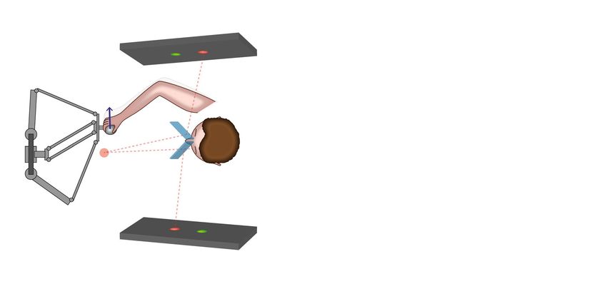
Figure 4. Comparison of hierarchical and non-hierarchical fitting algorithms. Parameter estimation quality for
our HMC hierarchical fitting procedure (orange), an HMC non-hierarchical fitting procedure (red), and a EM
fitting procedure45 (blue). For each random parameter setting of the surrogate two-state datasets, we represent
the error in parameter reconstruction (estimated minus set parameter) for each fitting procedure, including
the distributions of the errors, average and 95% confidence intervals of the squared error; and the correlation
(average d 95% CI) between the estimated and set parameters (CC).
Scientific Reports | (2022) 12:10198 | https://doi.org/10.1038/s41598-022-13866-y 8
Vol:.(1234567890)www.nature.com/scientificreports/
Figure 5. Comparison of two-state model parameters between the perturbation planes. (A) Estimated fast and
slow retention (af ,jp , as,jp), learning rates (bf ,jp , bs,jp), and measurement and planning variabilities (σx,jp, σu,jp)
for the sagittal (S), horizontal (H) and coronal (C) perturbation planes. Each color represents one subject. The
error bars correspond to 95% credible intervals (i.e., contain 95% of the posterior probability) for the population
average hyper-parameters µas ,p , µaf ,p , µbs ,p , µbf ,p , µσx ,p , µσu ,p. The steady-state Kalman gain K was
computed from the posteriors of the measurement noise and planning noise. (B) Relationships between the slow
learning rate bs and variability related parameters: measurement noise variability, planning noise variability, and
steady-state Kalman gain. Points correspond to individual subjects’ parameters in the different rotation planes
(coded by color). The correspondingly colored lines represent linear fits based on the across-subject parameter
values within each plane. The grey line corresponds to a linear fit based on subjects’ parameters values across
all planes. The horizontal and vertical error bars correspond to 95% credible intervals for the corresponding
parameter population average hyper-parameters.
sagittal-horizontal = 0.0213). These results indicate that we can assume with a high level of certainty (> 95%)
that the learning coefficients differs among the perturbation types. To test if the above-mentioned mechanism
of OI can explain the observed differences between the perturbed planes in our experiment, we also correlated
planning and measurement variabilities with the slow learning rate bs for each experimental run in our dataset
(Fig. 5B). Correlations between planning variability and the learning rate, as well as between measurement
variability and learning rate, were low (respective R2: 0.13 and 0.11), but with a trend consistent to the OI pre-
dictions, i.e., low measurement noise and high planning noise correlate with higher values of the slow learning
rate. When combining the contribution of the two noise parameters into an estimate of a Kalman gain for each
subject, the slow learning rate was explained much better (R2 between K and bs: 0.48), with a high Kalman gain
being associated with high learning rate. Notably, this correlation between Kalman gain (K) and slow learning
rate (bs) is determined by the different levels for K and bs between the perturbation planes. This means, the slow
learning rate is mostly explained by the plane of the workspace in which the perturbation is applied (R2 = 0.94),
while it does not correlate with the Kalman gain variation across the individual subjects within a perturbation
condition. Last, the fast learning component shows a correlation with the Kalman gain among perturbed planes
(R2 between K and bf: 0.34).
A long washout plus additional waiting time between conditions prevented savings or anterograde effects
when switching between different planes of perturbation. To test for this, a forward stepwise linear regression
was used to identify possible predictors of the learning rates (bf or bs independently) out of the order of execu-
tion (1st executed task, 2nd execution task or 3rd executed task) and perturbed axis. At each step, variables were
added based on p-values < 0.05. For both learning rates bs and bf, only the perturbed axis was added to the model
with p = 2.98E−44 and p = 8.22E−14 respectively. This means that we did not observe a significant contribution
of savings or anterograde effects on the learning rates.
Since the task uses multiple reach targets, one separate model could be fitted for each target unless one
assumes full generalization between sequentially visited targets. To avoid this pitfall and corresponding increase
in complexity, we fitted the model using epochs, motivated by the fact that in each epoch each target was visited
one time. When we also tested the model for the case where full generalization happens between two consecutives
Scientific Reports | (2022) 12:10198 | https://doi.org/10.1038/s41598-022-13866-y 9
Vol.:(0123456789)www.nature.com/scientificreports/
Figure 6. Recovery of simulated correlations between model parameters by the HMC algorithm. (A) A
correlation among bs and K was introduced in the surrogate data by setting bs equal to 0.3 times K (dashed
black line). (B) When no correlation between bs and K was added to the surrogate data, the HMC fitting
algorithm did not introduce artificial spurious correlations.
targets, we found similar results as for the model trained on epochs (R2 between K and bs: 0.29, Supplementary
Fig. 4).
We also validated the ability of our method to extract correlated learning parameters whenever present. For
this, we simulated an additional set of data where the slow learning rate bs was imposed to be 0.3 times the steady-
state Kalman gain (see Methods). Figure 6A shows that we were able to reconstruct such correlation with our
method. Conversely, when no correlation between the slow learning rate and the Kalman gain was introduced
in the dataset, the method does not introduce spurious correlation. Figure 6 overall confirms the validity of our
method for the study of correlations between two-state model parameters.
Discussion
We tested if observations and model assumptions about optimal integration (OI) theory for motor learning, as
previously derived from one- or two-dimensional highly confined reach tasks, also hold true for largely uncon-
strained movements in three-dimensional space. We show that the rate of visuomotor adaptation under 3D
stereoscopic vision depends on the plane in which a 2D visuomotor rotation perturbation is applied. Subjects
adapted best to perturbations in the coronal plane followed by sagittal and horizontal planes. The rates of slow
and fast learning correlated well with the Kalman gain when considering the variation across perturbation con-
ditions, but not across subjects within a condition. We could separately assess the within and across condition
parameters with our novel hierarchical Bayesian HMC fitting of the data. These results show that important
aspects of OI theories of motor control derived from 2D movements generalize to the largely unconstrained 3D
movements studied here, at least at the average population level, but do not extend to the individual subject level
for any of the applied perturbations12.
A novel two‑state hierarchical HMC algorithm for precise estimation of motor learning param-
eters. We developed a novel HMC Bayesian fitting procedure with a multilevel hierarchical structure to take
into account effects from multiple subjects performing a motor adaptation task in three different learning con-
ditions, i.e., when different planes relative to the body were perturbed. Naturally, such a hierarchical approach
shows lower goodness-of-fit to single-subject adaptation curves than algorithms that focus on single-subject
data since the hyper-parameter at the population level (i.e. all the samples coming from a same distribution) act
as regularization term. But multi-subject experiments are typically designed to determine the effects of experi-
mental variations on the motor learning behavior independent of test subject. Hence, it is most important to best
estimate the underlying learning parameters.
For the current experimental design, our procedure is better able to reconstruct actual model parameters
than a state-of-the-art EM fitting algorithm45 or a non-hierarchical Bayesian HMC model, as revealed from the
surrogate testing. This is due to the low identifiability of such two-state models for relatively short adaptation
experiments comprising only dozens or few hundreds of trials per condition. The low identifiability is a result of
random fluctuations in the shape of the adaptation curve and is easily associated with various learning param-
eters. In the hierarchical model, each parameter is sampled from a population-level distribution, the parameters
of which are also part of the model. This makes extreme values for the reconstructed parameter less likely.
Using our hierarchical model, we show that a two-state model fits the data significantly better than a single-
state model. The two-state model is well established for subjects performing in a 2D e nvironment7,37 and better
explains learning mechanisms such as savings and anterograde interference in 2D settings38. As previously
hypothesized4,6, the fast learning process could be partly associated to an explicit process and the slow learning
Scientific Reports | (2022) 12:10198 | https://doi.org/10.1038/s41598-022-13866-y 10
Vol:.(1234567890)www.nature.com/scientificreports/
process to an implicit process, both with anatomically distinct associated brain a reas6,20,43. While it is plausible
to assume that an interplay of explicit and implicit learning mechanisms is independent of the dimensionality
of the task, to our knowledge, the two-state model to date has not been demonstrated for adaptation paradigms
involving 3D movements. If one accepts the association of fast state with explicit learning and slow state with
implicit learning then the fact that we found a two-state model to better fit the adaptation data than a single-
state model, without having used a paradigm that explicitly enforces two-states dynamics (like re-learning after
washout trials37), would indicate that the explicit learning component is more pronounced in our 3D compared
to classic two-dimensional paradigms. This finding is also in line with a recent study showing that VR visuomotor
rotation tasks have a stronger explicit component than non-VR tasks8. Last, despite the general assumptions that
two-states model better explains phenomena like savings and anterograde interference than one-state models, a
novel modelling framework56 taking into account the context where learning happens has been recently showed
to better account for these phenomena than two-state models.
Differences in estimated planning and measurement noises explain differences in learning
rate. Motor learning studies are informative for motor rehabilitation protocols for patients that need to
relearn or re-adapt existing motor schemes. These patients will necessarily perform their movements in a three-
dimensional environment57–60. In our experiment, subjects adapted best to perturbations in the coronal plane,
followed by sagittal and horizontal planes. Differences in the slow and fast learning rates between the planes
were associated with different adaptation levels that were achieved during perturbation trials in our data. In the
following, we will discuss how these anisotropies in adaptation are related to anisotropies in estimated planning
and measurement noise, and, hence, could be explained by effects of gravity and depth perception, respectively.
The fact that adaptation is slowest in the horizontal plane likely is explained by an anisotropy in planning
variability resulting from gravity. Previous studies suggested that movements along the vertical dimension have a
higher level of planning variability associated with gravity compensation33–36. Optimally combining uncertainties
on planning together with uncertainties on the estimation of the effector position here then means that sensory
measurements should be given more credibility in vertical movements due to the higher planning variability.
This leads to the prediction that adaptive corrections in the horizontal plane should arise slower than corrections
in the sagittal or coronal plane, since the latter contain the vertical dimension with the higher measurement
credibility. Consistent with this view, perturbations in the horizontal plane in our data were associated with the
slowest adaptation rates and lowest estimates of planning variability, while estimated measurement variability
in the horizontal plane was close to the coronal plane (Fig. 5B).
The fact that adaptation is fastest in the coronal plane likely is explained by anisotropies in measurement
variability resulting from visual depth perception. In our model, measurement noise represents the reliability of
the subject’s measurements of the cursor position, i.e., the visual feedback about the movement. Subjects have
to rely mainly on stereoscopy to estimate visual depth and visual localization is less precise in depth15,32. Since
depth is not perturbed by a rotation in the coronal plane, measurement error is least in the coronal condition
and adaptation should be faster compared to visuomotor rotations in the sagittal and horizontal planes which
both resulted in perturbations of cursor depth. Consistent with this view, perturbations in the coronal plane were
associated with the fastest adaptation rates and lowest estimates of measurement noise (Fig. 5B). Corresponding
to this, other studies showed that subjects tend to adapt worse when the measurement variability (or sensory
noise) was higher due to blurred error f eedback11,14,21.
Final adaptation levels in our experiment tended to be lower than reported in the literature for 2D paradigms
(see for e xample61). Whether this was due to higher complexity of 3D movements and/or more difficult 3D target
and cursor localization is unclear. Adaptation experiments with movements being constrained to the coronal
plane but otherwise using the same apparatus yielded higher adaptation levels in line with values reported by
others (data not shown). Therefore, we think that the increased measurement variability of our experimental
setting explains why we observe lower adaptation than standard adaptation experiments with expected lower
measurement variability. In addition, it is possible that the generalization of adaptation among targets in our 3D
space is reduced when compared to 2D movements and therefore lower adaptation rates have to be expected.
Optimal integration theory in 3D. Previous studies11,12,21,26,31, provided evidence for the OI theory dur-
ing visuomotor adaptation. They showed that the planning component of motor noise correlates positively with
the adaptation rate while the measurement component correlates negatively, at least when the respective noise
component is experimentally kept constant. While the adaptation data from our 3D movements yielded similar
trends, the correlation of slow learning rate with either measurement or planning variability was weak. For an
optimal learner, the Kalman gain is indicative of the level of correction attributed to the experienced error11,21,31.
This Kalman gain positively correlates with the slow learning rate in our data, supporting the idea that subjects
optimally integrate the information relative to the internal state with experienced (visual) feedback. However,
and as opposed to what was suggested in previous s tudies12,31, we observe the correlation between Kalman gain
and learning rate only across different perturbation conditions. Within each perturbation condition and across
individual subjects, there was no correlation between Kalman gain and learning rate.
One speculative reason for not observing this relationship is that in our experimental settings the ranges of
measured learning rates (bs) are mainly determined by the plane of adaptation (Fig. 5B). It could be, that in our
case, the higher measurement uncertainty of 3D adaptive movements affected the learning rate at the level that
single subject differences could not any longer be observed.
Scientific Reports | (2022) 12:10198 | https://doi.org/10.1038/s41598-022-13866-y 11
Vol.:(0123456789)www.nature.com/scientificreports/
Conclusion
Here, we develop a novel HMC fitting procedure to correlate learning rates and noise levels estimated with the
same model and without the need to experimentally manipulating these error variabilities. By applying this model
to a sensorimotor adaptation task with naturalistic movements in 3D, we found that the rate of adaptation with
which subjects counteract applied visuomotor rotations, depends on the statistics of the combined errors with
which subjects plan and perceive movements. These errors differ between different axes relative to the body,
likely due to gravity compensation during planning- and perception-induced anisotropies. This insight could be
used in motor rehabilitation strategies by specifically targeting the orientation of the body relative to the target
while performing reaching movements to accelerate learning.
Data availability
The datasets used and/or analysed during the current study available from the corresponding author on reason-
able request.
Received: 7 March 2022; Accepted: 30 May 2022
References
1. Krakauer, J. W. Motor learning and consolidation: The case of visuomotor rotation. Adv. Exp. Med. Biol. 629, 405–421. https://doi.
org/10.1007/978-0-387-77064-2_21 (2009).
2. Leow, L. A., de Rugy, A., Marinovic, W., Riek, S. & Carroll, T. J. Savings for visuomotor adaptation require prior history of error,
not prior repetition of successful actions. J. Neurophysiol. 116, 1603–1614. https://doi.org/10.1152/jn.01055.2015 (2016).
3. Mazzoni, P. & Krakauer, J. W. An implicit plan overrides an explicit strategy during visuomotor adaptation. J. Neurosci. 26,
3642–3645. https://doi.org/10.1523/JNEUROSCI.5317-05.2006 (2006).
4. McDougle, S. D., Bond, K. M. & Taylor, J. A. Explicit and implicit processes constitute the fast and slow processes of sensorimotor
learning. J. Neurosci. 35, 9568–9579. https://doi.org/10.1523/JNEUROSCI.5061-14.2015 (2015).
5. Morehead, J. R., Qasim, S. E., Crossley, M. J. & Ivry, R. Savings upon re-aiming in visuomotor adaptation. J. Neurosci. 35, 14386–
14396. https://doi.org/10.1523/JNEUROSCI.1046-15.2015 (2015).
6. Taylor, J. A., Krakauer, J. W. & Ivry, R. B. Explicit and implicit contributions to learning in a sensorimotor adaptation task. J.
Neurosci. 34, 3023–3032. https://doi.org/10.1523/JNEUROSCI.3619-13.2014 (2014).
7. Wolpert, D. M., Diedrichsen, J. & Flanagan, J. R. Principles of sensorimotor learning. Nat. Rev. Neurosci. 12, 739–751. https://doi.
org/10.1038/nrn3112 (2011).
8. Anglin, J. M., Sugiyama, T. & Liew, S. L. Visuomotor adaptation in head-mounted virtual reality versus conventional training. Sci.
Rep. 7, 45469. https://doi.org/10.1038/srep45469 (2017).
9. Choi, W., Lee, J., Yanagihara, N., Li, L. & Kim, J. Development of a quantitative evaluation system for visuo-motor control in
three-dimensional virtual reality space. Sci. Rep. 8, 13439. https://doi.org/10.1038/s41598-018-31758-y (2018).
10. Lefrancois, C. & Messier, J. Adaptation and spatial generalization to a triaxial visuomotor perturbation in a virtual reality environ-
ment. Exp. Brain Res. 237, 793–803. https://doi.org/10.1007/s00221-018-05462-2 (2019).
11. Burge, J., Ernst, M. O. & Banks, M. S. The statistical determinants of adaptation rate in human reaching. J. Vis. 8(20), 19–21. https://
doi.org/10.1167/8.4.20 (2008).
12. van der Vliet, R. et al. Individual differences in motor noise and adaptation rate are optimally related. eNeuro https://doi.org/10.
1523/ENEURO.0170-18.2018 (2018).
13. Ernst, M. O. & Banks, M. S. Humans integrate visual and haptic information in a statistically optimal fashion. Nature 415, 429–433.
https://doi.org/10.1038/415429a (2002).
14. Kording, K. P. & Wolpert, D. M. Bayesian integration in sensorimotor learning. Nature 427, 244–247. https://doi.org/10.1038/
nature02169 (2004).
15. van Beers, R. J., Wolpert, D. M. & Haggard, P. When feeling is more important than seeing in sensorimotor adaptation. Curr. Biol.
12, 834–837. https://doi.org/10.1016/s0960-9822(02)00836-9 (2002).
16. Wolpert, D. M. & Ghahramani, Z. Computational principles of movement neuroscience. Nat. Neurosci. 3(Suppl), 1212–1217.
https://doi.org/10.1038/81497 (2000).
17. Friston, K. What is optimal about motor control?. Neuron 72, 488–498. https://doi.org/10.1016/j.neuron.2011.10.018 (2011).
18. Scott, S. H. Optimal feedback control and the neural basis of volitional motor control. Nat. Rev. Neurosci. 5, 532–546. https://doi.
org/10.1038/nrn1427 (2004).
19. Shadmehr, R. & Krakauer, J. W. A computational neuroanatomy for motor control. Exp. Brain Res. 185, 359–381. https://doi.org/
10.1007/s00221-008-1280-5 (2008).
20. Shadmehr, R., Smith, M. A. & Krakauer, J. W. Error correction, sensory prediction, and adaptation in motor control. Annu. Rev.
Neurosci. 33, 89–108. https://doi.org/10.1146/annurev-neuro-060909-153135 (2010).
21. Wei, K. & Kording, K. Uncertainty of feedback and state estimation determines the speed of motor adaptation. Front. Comput.
Neurosci. 4, 11. https://doi.org/10.3389/fncom.2010.00011 (2010).
22. Cheng, S. & Sabes, P. N. Modeling sensorimotor learning with linear dynamical systems. Neural. Comput. 18, 760–793. https://
doi.org/10.1162/089976606775774651 (2006).
23. Cheng, S. & Sabes, P. N. Calibration of visually guided reaching is driven by error-corrective learning and internal dynamics. J.
Neurophysiol. 97, 3057–3069. https://doi.org/10.1152/jn.00897.2006 (2007).
24. Korenberg, A. & Ghahramani, Z. A Bayesian view of motor adaptation. Cahiers de Psychologie Cognitive 21, 537–564 (2002).
25. Morel, P. D. & Baraduc, P. in Cinquième conférence plénière française de Neurosciences Computationnelles, "Neurocomp’10" (2010).
26. van Beers, R. J. Motor learning is optimally tuned to the properties of motor noise. Neuron 63, 406–417. https://doi.org/10.1016/j.
neuron.2009.06.025 (2009).
27. Diedrichsen, J., Shadmehr, R. & Ivry, R. B. The coordination of movement: Optimal feedback control and beyond. Trends Cogn.
Sci. 14, 31–39. https://doi.org/10.1016/j.tics.2009.11.004 (2010).
28. Kalman, R. E. A new approach to linear filtering and prediction problems. J. Basic Eng. 82, 35–45. https://doi.org/10.1115/1.36625
52 (1960).
29. Baddeley, R. J., Ingram, H. A. & Miall, R. C. System identification applied to a visuomotor task: Near-optimal human performance
in a noisy changing task. J. Neurosci. 23, 3066–3075 (2003).
30. Ghahramani, Z., Wolptrt, D. M. & Jordan, M. I. in Advances in Psychology Vol. 119 (eds Morasso, P. & Sanguineti, V.) 117–147
(North-Holland, 1997).
31. He, K. et al. The statistical determinants of the speed of motor learning. PLoS Comput. Biol. 12, e1005023. https://doi.org/10.1371/
journal.pcbi.1005023 (2016).
Scientific Reports | (2022) 12:10198 | https://doi.org/10.1038/s41598-022-13866-y 12
Vol:.(1234567890)You can also read