Uncertainty quantification using martingales for misspecified Gaussian processes
←
→
Page content transcription
If your browser does not render page correctly, please read the page content below
Proceedings of Machine Learning Research vol 132:1–20, 2021   32nd International Conference on Algorithmic Learning Theory

                                                                Uncertainty quantification using martingales
                                                                    for misspecified Gaussian processes
                                          Willie Neiswanger                                                              NEISWANGER @ CS . STANFORD . EDU
                                          Stanford University
                                          Aaditya Ramdas                                                                          ARAMDAS @ STAT. CMU . EDU
                                          Carnegie Mellon University
arXiv:2006.07368v2 [stat.ML] 2 Mar 2021

                                          Editors: Vitaly Feldman, Katrina Ligett, and Sivan Sabato

                                                                                                  Abstract
                                               We address uncertainty quantification for Gaussian processes (GPs) under misspecified priors, with
                                               an eye towards Bayesian Optimization (BO). GPs are widely used in BO because they easily enable
                                               exploration based on posterior uncertainty bands. However, this convenience comes at the cost of
                                               robustness: a typical function encountered in practice is unlikely to have been drawn from the data
                                               scientist’s prior, in which case uncertainty estimates can be misleading, and the resulting exploration
                                               can be suboptimal. We present a frequentist approach to GP/BO uncertainty quantification. We
                                               utilize the GP framework as a working model, but do not assume correctness of the prior. We instead
                                               construct a confidence sequence (CS) for the unknown function using martingale techniques. There
                                               is a necessary cost to achieving robustness: if the prior was correct, posterior GP bands are narrower
                                               than our CS. Nevertheless, when the prior is wrong, our CS is statistically valid and empirically
                                               outperforms standard GP methods, in terms of both coverage and utility for BO. Additionally, we
                                               demonstrate that powered likelihoods provide robustness against model misspecification.

                                          1. Introduction
                                          In Bayesian optimization (BO), a Bayesian model is leveraged to optimize an unknown function f ∗
                                          (Mockus et al., 1978; Shahriari et al., 2015; Snoek et al., 2012). One is allowed to query the function
                                          at various points x in the domain, and get noisy observations of f ∗ (x) in return. Most BO methods
                                          use a Gaussian process (GP) prior, with a chosen kernel function. However, in practice, it may be
                                          difficult to specify the prior accurately. A few examples of where misspecification may arise include
                                             • an incorrect kernel choice (e.g. squared exponential versus Matern),
                                             • bad estimates of kernel hyperparameters (e.g. lengthscale or signal variance), and
                                             • heterogenous smoothness of f ∗ over the domain X .
                                          Each of these can yield misleading uncertainty estimates, which may then negatively affect the
                                          performance of BO (Schulz et al., 2016; Sollich, 2002). This paper instead presents a frequentist
                                          approach to uncertainty quantification for GPs (and hence for BO), which uses martingale tech-
                                          niques to construct a confidence sequence (CS) for f ∗ , irrespective of misspecification of the prior. A
                                          CS is a sequence of (data-dependent) sets that are uniformly valid over time, meaning that {Ct }t≥1
                                          such that Pr(∃t ∈ N : f ∗ ∈ / Ct ) ≤ α. The price of such a robust guarantee is that if the prior was
                                          indeed accurate, then our confidence sets are looser than those derived from the posterior.
                                              Outline The next page provides a visual illustration of our contributions. Section 2 provides
                                          the necessary background on GPs and BO, as well as on martingales and confidence sequences.
                                          Section 3 derives our prior-robust confidence sequence, as well as several technical details needed to
                                          implement it in practice. Section 4 describes the simulation setup used in Figure 1 in detail. We end
                                          by discussing related work and future directions in Section 5, with additional figures in the appendix.

                                          © 2021 W. Neiswanger & A. Ramdas.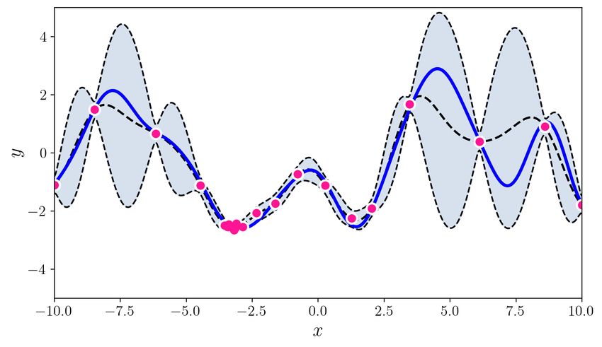
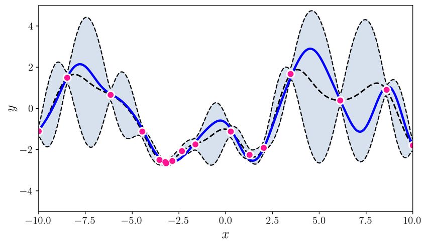
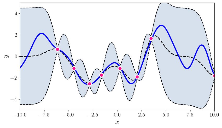
U NCERTAINTY QUANTIFICATION USING MARTINGALES FOR MISSPECIFIED G AUSSIAN PROCESSES

Figure 1: This figure summarizes the paper’s contributions. The top two plots show various random functions
drawn from a GP prior with hyperparameter settings A (left) and B (right). Then, a single function (blue
curve) is drawn using prior A, and is fixed through the experiment. The pink dots are the observations;
there are 3, 5, 10, 20, 30, 60 pink dots in the bottom 6 plots. The grey shaded region shows the standard
GP posterior when (mistakenly) working with prior B. The brown shaded region shows our new confidence
sequence, also constructed with the wrong prior B. The brown region is guaranteed to contain the true function
with high probability uniformly over time. The grey confidence band after just 3 observations is already
(over)confident, but quite inaccurate, and it never recovers. The brown confidence sequence is very wide
early on (perhaps as it should be) but it recovers as more points are drawn. Thus, the statistical price of
robustness to prior misspecification is wider bands. Whether this is an acceptable tradeoff to the practitioner
is a matter of their judgment and confidence in the prior. The observation that the posterior never converges
to the truth (the data does not wash away the wrong prior) appears to be a general phenomenon of failure
of the Bernstein-von-Mises theorem in infinite dimensions (Freedman, 1999; Cox, 1993). The rest of this
paper explains how this confidence sequence is constructed, using the theory of martingales. We provide more
details (such as kernel hyperparameters A and B) for this simulation in Section 4. Simulations for BO are
available in the supplement.                          2
U NCERTAINTY QUANTIFICATION USING MARTINGALES FOR MISSPECIFIED G AUSSIAN PROCESSES

2. Mathematical background
Gaussian Processes (GP). A GP is a stochastic process (a collection of random variables indexed
by domain X ) such that every finite collection of those random variables has a multivariate normal
distribution. The distribution of a GP is a distribution over functions g : X 7→ R, and thus GPs are
often used as Bayesian priors over unknown functions. A GP is itself typically specified by a mean
function µ : X → R and a covariance kernel κ : X 2 → R. Suppose we draw a function

                                              f ∼ GP(µ, κ)                                              (1)

and obtain a set of n observations Dn = {(Xi , Yi )}ni=1 , where Xi ∈ X ,

                              Yi = f (Xi ) + i ∈ R, and i ∼ N (0, η 2 ).                              (2)

Then, the posterior process f |Dn is also a GP with mean function µn and covariance kernel κn ,
described as follows. Collect the Yi s into a vector Y ∈ Rn , and define k, k 0 ∈ Rn with ki =
κ(x, Xi ), ki0 = κ(x0 , Xi ), and K ∈ Rn×n with Ki,j = κ(Xi , Xj ). We can then write µn , κn as

          µn (x) = k > (K + η 2 I)−1 Y,         κn (x, x0 ) = κ(x, x0 ) − k > (K + η 2 I)−1 k 0 .       (3)

Further background on GPs can be found in Williams and Rasmussen (2006). In this paper, we
describe a simple method for inference when (1) does not hold, but (2) holds; in other words, the
prior is arbitrarily misspecified but the model is correct. (If both are correct, GPs work fine, and if
both are arbitrarily misspecified, statistical inference is essentially impossible.)
Bayesian Optimization (BO). Suppose we wish to minimize an unknown, fixed, nonrandom,
function f ∗ over a domain X . Bayesian optimization (BO) leverages probabilistic models to perform
optimization by assuming that f ∗ was sampled from a GP.
     At time t (we switch from n to t to emphasize temporality), assume we have already evaluated
f ∗ at points {Xi }t−1                                  t−1
                    i=1 and obtained observations {Yi }i=1 . To determine the next domain point Xt
to evaluate, we first use the posterior GP to define an acquisition function ϕt : X → R, which
specifies the utility of evaluating f ∗ at any x ∈ X . We then minimize the acquisition function to
yield Xt = argminx∈X ϕt (x), and evaluate f ∗ at Xt . One of the most commonly used acquisition
functions is the GP lower confidence bound1 (GP-LCB) by Srinivas et al. (2010), written
                                                           1/2
                                      ϕt (x) = µt (x) − βt σt (x)                                       (4)

where µt and σt are the posterior GP mean and standard deviation, and βt > 0 is a tuning parameter
that determines the tradeoff between exploration and exploitation.
    Due to inheriting their worldview from GPs, theoretical guarantees in the BO literature typically
assume correctness of both (1) and (2). These may or may not be reasonable assumptions. In this
paper, (1) is used as a working model that is not assumed correct, but (2) is still assumed. We do not
provide guarantees on any particular BO algorithm persay, but instead provide correct uncertainty
quantification that could be exploited by any BO algorithm, including but not necessarily GP-LCB.
 1. Often described as the GP upper confidence bound (GP-UCB), we use the GP lower confidence bound (GP-LCB)
    since we are performing minimization.

                                                     3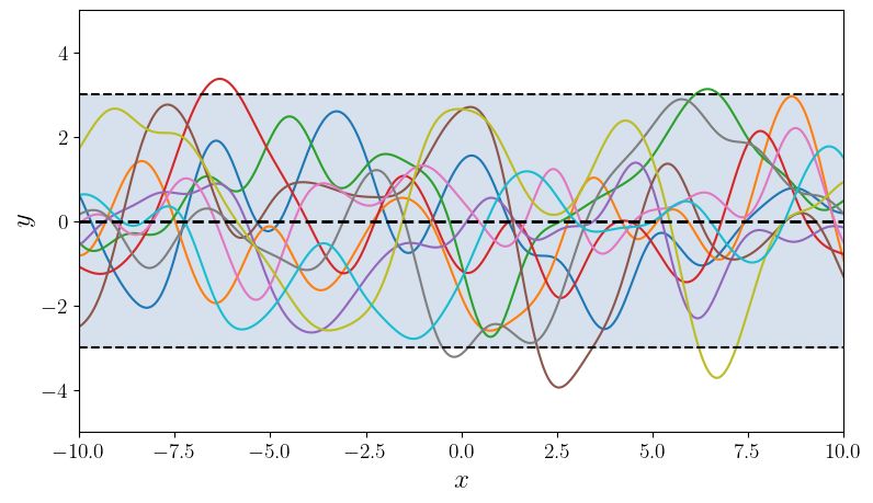
U NCERTAINTY QUANTIFICATION USING MARTINGALES FOR MISSPECIFIED G AUSSIAN PROCESSES

Filtrations and stopping times. To make the sequential aspect of BO explicit, let

                                Dt = σ((X1 , Y1 ), . . . , (Xt , Yt )) ≡ σ(Dt )

denote the sigma-field of the first t observations, which captures the information known at time t; D0
is the trivial sigma-field. Since Dt ⊃ Dt−1 , {Dt }t≥0 forms a filtration (an increasing sequence of
sigma-fields). Using this language, the acquisition function ϕt is then predictable, written ϕt ∈ Dt−1 ,
meaning that it is measurable with respect to Dt−1 and is hence determined with only the data
available after t − 1 steps. As a result, Xt is technically also predictable. However, Yt is not
predictable (it is adapted), since Yt ∈ Dt but Yt ∈ / Dt−1 . A stopping time τ is an N-valued random
variable such that {τ ≥ t} ∈ Dt−1 for all t, or equivalently if

                                               {τ ≤ t} ∈ Dt ,

meaning that we can tell if we have stopped by time t, using only the information available up to t.
Martingales. An integrable process {Mt }t≥0 is said to be a martingale with respect to filtration
{Dt }t≥0 , if Mt ∈ Dt and for every t ≥ 1, we have

                                            E[Mt |Dt−1 ] = Mt−1 .

If we replaced the = above by an inequality ≤, the resulting process is called a supermartingale.
Every martingale is a supermartingale but not vice versa. Ville’s inequality (Ville, 1939, Pg. 100)
states that if {Mt } is a nonnegative supermartingale, then for any x > 0, we have
                                                                E[M0 ]
                                        Pr(∃t ∈ N : Mt ≥ x) ≤          .                            (5)
                                                                  x
See Howard et al. (2020, Lemma 1) for a measure-theoretic proof and Shafer and Vovk (2019,
Proposition 14.8) for a game-theoretic variant. In many statistical applications, M0 is chosen to
deterministically equal one. Ville’s may be viewed as a time-uniform version of Markov’s inequality
for nonnegative random variables. In the next section, we will construct a martingale (hence
supermartingale) for GP/BO, and construct a confidence sequence (defined next) for the underlying
function f by applying Ville’s inequality.
Confidence sequences (CS). Suppose we wish to sequentially estimate an unknown quantity θ∗
(a scalar, vector, function, etc.) as we observe an increasing number of datapoints, summarized as a
filtration Dt . A CS is defined as a sequence of confidence sets {Ct }t≥1 that contains θ∗ at all times
with high probability. Formally, for a confidence level α ∈ (0, 1), we need that Ct ∈ Dt and

                 Pr(∀t ∈ N : θ∗ ∈ Ct ) ≥ 1 − α            ≡   Pr(∃t ∈ N : θ∗ ∈
                                                                             / Ct ) ≤ α.            (6)
                 |       {z         }                         |       {z         }
                    coverage at all times                          error at some time

Here, Ct obviously depends on α, but it is suppressed for simplicity. Importantly, property (6) holds
if and only if Pr(θ∗ ∈ Cτ ) ≥ 1 − α for all possible (potentially infinite) stopping times τ . This
allows us to provide correct uncertainty quantification that holds even at data-dependent stopping
times. Next, we describe our construction of a confidence sequence for f ∗ .

                                                      4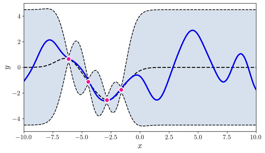
U NCERTAINTY QUANTIFICATION USING MARTINGALES FOR MISSPECIFIED G AUSSIAN PROCESSES

3. Deriving our prior-robust confidence sequence
One of the roles of the prior in BO is to restrict the complexity of the function f ∗ . Since we do not
assume the prior is well-specified, we need some other way to control the complexity of f ∗ —without
any restriction on f ∗ , we cannot infer its value at any point outside of the observed points since it
could be arbitrarily different even at nearby points. We do this by assuming that f ∗ ∈ F for some
F, that is either explicitly specified—say via a bound on the Reproducing Kernel Hilbert Space
(RKHS) norm, or by a bound on the Lipschitz constant—or implicitly specified (via some kind of
regularization).
    The choice of F has both statistical and computational implications; the former relates to the
size of the class, the sample complexity of identifying the optimum via BO, and the rate at which the
confidence bands will shrink, while the latter relates to how much time it takes to calculate and/or
update the confidence bands. Ultimately, F must be specified by the practitioner based on their
knowledge of the underlying problem domain. For this section, we treat any arbitrary F, and in the
next section we discuss one particular choice of F for which the computational load is reasonable.
    It is worth noting that we have not simply shifted the problem from specifying a prior to specifying
F—the latter does not impose a probability structure amongst its elements, while the former does.
There are other differences as well; for example comparing a GP prior with a particular kernel, to a
bounded RKHS ball for the same kernel, we find that the former is much richer than the latter—as
mentioned after Theorem 3 of Srinivas et al. (2010), random functions drawn from a GP have infinite
RKHS norm almost surely, making the sample paths much rougher/coarser than functions with
bounded RKHS norm.

3.1. Constructing the prior-posterior-ratio martingale
We first begin with some technicalities. Recall that a GP is interpreted as a prior distribution over
functions g : X 7→ R. For simplicity, and to avoid measure-theoretic issues, consider the case of
X = Rd by default, equipped with the Borel sigma algebra. It is clear to us that the following results
do hold more generally, albeit at the price of further mathematical machinery, since extra care is
needed when dealing with infinite-dimensional measures. Let GP0 (f ) represent the prior “density”
at function f , and let GPt (f ) represent the posterior “density” at f after observing t datapoints.
“Density” is in quotes because in infinite dimensional spaces, there is no analog of the Lebesgue
measure, and thus it is a priori unclear which measure these are densities with respect to. Proceeding
for now, we soon sort this issue out.
    Define the prior-posterior-ratio for any function f as the following real-valued process:
                                                       GP0 (f )
                                         Rt (f ) :=             .                                   (7)
                                                       GPt (f )
Note that R0 (f ) = 1 for all f . Denote the working likelihood of f by
                               t                Y −f (X ) 2   t
                                                                      Yi − f (Xi )

                             Y      1     − 12 i η i
                                                              Y 1
                 Lt (f ) :=        √ e                      ≡     φ                  ,              (8)
                                  η 2π                          η          η
                             i=1                                i=1

where φ(y) denotes the standard Gaussian PDF, so that φ((y − µ)/σ)/σ is the PDF of N (µ, σ 2 ).
Then, for any function f , the working posterior GP is given by
                                                 GP0 (f )Lt (f )
                                    GPt (f ) := R                 .                                 (9)
                                                  g GP0 (g)Lt (g)

                                                   5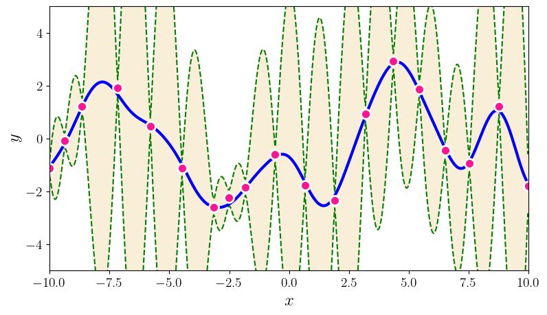
U NCERTAINTY QUANTIFICATION USING MARTINGALES FOR MISSPECIFIED G AUSSIAN PROCESSES
Substituting the posterior (9) and likelihood (8) into the definition of the prior-posterior-ratio (7), the
latter can be more explicitly written as
Lt (g) Lt (g)
Z
Rt (f ) = GP0 (g) ≡ Eg∼GP0 , (10)
g Lt (f ) Lt (f )
and it is this last form that we use, since it avoids measure-theoretic issues. Indeed, Lt (f ), Rt (f ) are
well-defined and finite for every f , as long as f itself is finite, and one is anyway uninterested in
considering functions that can be infinite on the domain.
As mentioned at the start of this section, fix a function f ∗ ∈ F. Assume that the data are observed
according to (2) when the Xi s are predictably chosen according to any acquisition function. Despite
not assuming (1), we will still use a GP framework to model and work with this data, and we call
this our “working prior” to differentiate it from an assumed prior.
Lemma 1. Fix any arbitrary f ∗ ∈ F, and assume data-generating model (2). Choose any acquisition
function ϕt , any working prior GP0 and construct the working posterior GPt . Then, the prior-
posterior-ratio at f ∗ , denoted {Rt (f ∗ )}t≥0 , is a martingale with respect to filtration {Dt }t≥0 .
Proof. Evaluating Rt at f ∗ , taking conditional expectations and applying Fubini’s theorem, yields
∗ Lt (g)
EDt ∼f ∗ [Rt (f ) | Dt−1 ] = EDt ∼f ∗ Eg∼GP0 | Dt−1
Lt (f ∗ )
Lt (g)
= Eg∼GP0 EDt ∼f ∗ | D t−1
Lt (f ∗ )
φ( Yt −g(X t)
)
(i) Lt−1 (g) η ∗
= Eg∼GP0
∗
· EDt ∼f ∗
Y −f ∗ (X ) | Dt−1
= Rt−1 (f ),
Lt−1 (f ) φ( t t
)
η
| {z }
=1
where equality (i) follows because Xt ∈ Dt−1 by virtue of the acquisition funtion being predictable.
To conclude the proof, we just need to argue that the braced term in the last expression equals one as
claimed. This term can be recognized as integrating a likelihood ratio, which equalsR one because
for
R any two absolutely continuous distributions P, Q, we have E P (dQ/dP ) = (dQ/dP )dP =
dQ = 1. For readers unfamiliar with this fact, we verify it below by direct integration. Once we
condition on Dt−1 , only Yt is random, and so the relevant term equals
Z φ( y−g(Xt ) )
y − f ∗ (Xt )
y − g(Xt )
Z
η 1 1
y−f ∗ (Xt ) η
φ dy = φ dy = 1,
y φ( ) η y η η
η
where the last equality holds simply because a Gaussian PDF with any mean integrates to one.
Also see Waudby-Smith and Ramdas (2020b) for another application of the prior-posterior ratio
martingale. The prior-posterior-ratio is related to the marginal likelihood and the Bayes factor, but
the latter two terms are typically used in a Bayesian context, so we avoid their use since the guarantee
above is fully frequentist: the expectation EDt ∼f ∗ is not averaging over any prior: no prior is even
assumed to necessarily exist in generating f ∗ , or if it exists it may be incorrectly specified. The most
6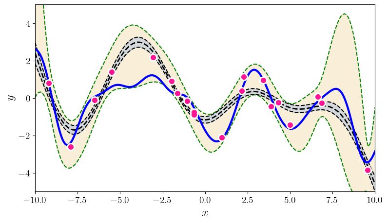
U NCERTAINTY QUANTIFICATION USING MARTINGALES FOR MISSPECIFIED G AUSSIAN PROCESSES

accurate analogy to past work in frequentist statistics is to interpret this statement as saying that the
mixture likelihood ratio is a martingale — a well known fact, implicit in Wald (1947), and exploited
in sequential testing (Robbins and Siegmund, 1970) and estimation (Howard et al., 2021). Here, the
prior GP0 plays the role of the mixing distribution. However, our language more directly speaks to
how one might apply Bayesian methodology towards frequentist goals in other problems.

3.2. Constructing the confidence sequence
Despite the apparent generality of Lemma 1, it is not directly useful. Indeed, Rt (f ∗ ) is a martingale,
but not Rt (f ) for any other f , and we obviously do not know f ∗ . This is where Ville’s inequality (5)
enters the picture: we use Lemma 1 to construct the following confidence sequence and use Ville’s
inequality to justify its correctness. Define

                                                               1
                                     Ct := f ∈ F : Rt (f ) <         .                              (11)
                                                              α

We claim that f ∗ is an element of the confidence set Ct , through all of time, with high probability.

Proposition 1. Consider any (fixed, unknown) f ∗ ∈ F that generates data according to (2), any
acquisition function ϕt , and any nontrivial working prior GP0 . Then, Ct defined in (11) is a
confidence sequence for f ∗ :
                                  Pr(∃t ∈ N : f ∗ ∈
                                                  / Ct ) ≤ α.
Thus, at any arbitrary data-dependent stopping time τ , we have Pr(f ∗ ∈
                                                                       / Cτ ) ≤ α.

Proof. First note that f ∗ ∈
                           / Ct if and only if Rt (f ∗ ) ≥ 1/α. Recall that Rt (f ∗ ) is a nonnegative
martingale by Lemma 1, and note that R0 (f ∗ ) = 1. Then, Ville’s inequality (5) with x = 1/α
implies that Pr(∃t ∈ N : Rt (f ∗ ) ≥ 1/α) ≤ α.

     Ct is our prior-robust confidence sequence for f ∗ . For the purposes of the following discussion,
let |Ct | denote its size, for an appropriate notion of size such as an -net covering. Intuitively, if the
working prior GP0 was accurate, which in the frequentist sense means that it put a large amount of
mass at f ∗ relative to other functions, then |Ct | will be (relatively) small. If the working prior GP0
was inaccurate, which could happen because of a poor choice of kernel hyperparameters, or a poor
choice of kernel itself, then |Ct | will be (relatively) large. This degradation of quality (|Ct | relative to
accuracy of the prior) is smooth, in the sense that as long as small changes in the GP hyperparameters
only change the mass at f ∗ a little bit, then the corresponding confidence sequence (and hence its
size) will also change only slightly. Formalizing these claims is possible by associating a metric over
hyperparameters, and proving that if the map from hyperparameters to prior mass is Lipschitz, then
the map |Ct | is also Lipschitz, but this is beyond the scope of the current work. Such “sensitivity
analysis” can be undertaken if the proposed new ideas are found to be of interest.
     Ct is a confidence band for the entire function f ∗ , meaning that it is uniform over both X and
time, meaning that it provides a confidence interval for f ∗ (x) that is valid simultaeously for all times
and for all x (on the grid, for simplicity). This uniform guarantee is important in practice because the
BO algorithm is free to query at any point, and also free to stop at any data-dependent stopping time.
     The aforementoned proposition should be compared to Srinivas et al. (2010, Theorem 6, Appendix
B), which is effectively a confidence sequence for f (though they did not use that terminology),
and yielded the regret bound in their Theorem 3, which is very much in the spirit of our paper.

                                                      7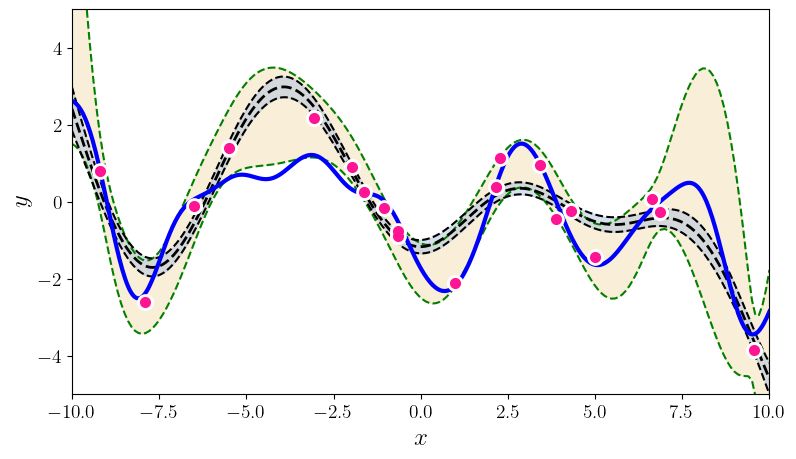
U NCERTAINTY QUANTIFICATION USING MARTINGALES FOR MISSPECIFIED G AUSSIAN PROCESSES

However, the constants in their Theorems 3, 6 are very loose, and it is our understanding that these
are never implemented as such in practice; in contrast, our confidence sequence is essentially tight,
with the error probability almost equaling α, because Ville’s inequality almost holds with equality
for nonnegative martingales (it would be exact equality in continuous time).
    Martingales have also been used in other fashions, for example to analyze convergence properties
of BO methods; for example, Bect et al. (2019) use (super)martingales to study consistency of
sequential uncertainty reduction strategies in the well-specified case.

4. Practical considerations and numerical simulations
Being an infinite dimensional confidence set containing uncountably many functions, even at a fixed
time, Ct cannot be explicitly stored on a computer. In order to actually use Ct in practice, two critical
questions remains: (a) returning to the very start of Section 3, how should we pick the set of functions
F under consideration? (b) at a fixed time t, and for a fixed new test point x under consideration by
the acquisition function for a future query, how can we efficiently construct the confidence interval
for f ∗ (x) that is induced by Ct ? These two questions are closely tied together: certain choices of F
in (a) may make step (b) harder. There cannot exist a single theoretically justified way of answering
question (a): the type of functions that are “reasonable” will depend on the application.
    We describe our approach to tackling these questions in the context of Figure 1. Our answer ties
together (a) and (b) using a form of implicit regularization; we suspect there is room for improvement.
Our code is available at: https://github.com/willieneis/gp-martingales

4.1. The introductory simulation
                                                                (1)                  (2)
In Figure 1, we define two gaussian processes priors, GP0 (µ1 , κ1 ) and GP0 (µ2 , κ2 ). Both
covariance matrices κ1 and κ2 are defined by a squared exponential kernel, i.e.
                                                     (x − x0 )2

                               κ(x, x0 ) = σ 2 exp −              ,                      (12)
                                                        2`2
with lengthscale ` and signal variance σ 2 . In this example, κ1 has parameters {` = 1, σ 2 = 1.5}
and κ2 has parameters {` = 3, σ 2 = 1}. Both GPs have a fixed noise variance η 2 = 0.1 in model
                                                                                    (1)
(2). We show the posterior 95% confidence region and posterior samples for GP0 (µ1 , κ1 ) and for
    (2)
GP0 (µ2 , κ2 ) in Figure 1; the top two plots show typical functions drawn from these priors.
                                                                      (1)
     Now, we draw a single function from the first prior, f ∗ ∼ GP0 (µ1 , κ1 ) shown as a blue line,
which we really treat as a fixed function in this paper. We then draw t observations from this function
via
                Xi ∼ Uniform [−10, 10] , Yi ∼ N f ∗ (Xi ), η 2 , i = 1, . . . , t.


                                                                        (2)
We compute the posterior GPt (Eq. 3), under the second prior GP0 (µ2 , κ2 ), and plot the 95%
confidence region for t ∈ (3, 5, 15, 17, 25, 40) in Figure 1, rows 2-4 (shown as blue shaded regions).
    We then aim to construct the prior-robust confidence sequence. For each t, we can write the
prior-posterior-ratio and confidence sequence for α = 0.05 as
                                   (2)
                               GP0 (f )
                     Rt (f ) =          , and Ct = {f ∈ F : Rt (f ) < 20} .                         (13)
                               GPt (f )

                                                   8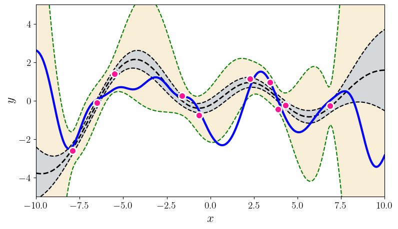
U NCERTAINTY QUANTIFICATION USING MARTINGALES FOR MISSPECIFIED G AUSSIAN PROCESSES

Next, we describe our procedure for implicitly specifying F while computing Ct in Section 4.2, and
plot it for each x ∈ [−10, 10] in Figure 1 (shown as yellow/brown shaded regions).

4.2. Implicit specification of F while computing the confidence interval for f ∗ (x) at time t
Suppose we are at iteration t of BO, using a Bayesian model with prior GP0 (µ0 , κ0 ). Assume that
we have observed data Dt−1 = {(Xi , Yi )}t−1                                    0   0
                                           i=1 . Assume we have a sequence X1 , X2 , ... ∈ X over
which we’d like to evaluate our acquisition function ϕt (x). In BO, this sequence would typically
be determined by an acquisition optimization routine, which we can view as some zeroth order
optimization algorithm. For each point X 0 in this sequence we do the following.
(1) Compute the GP posterior. Let Gt = {X ∈ Dt−1 } ∪ X 0 . We will restrict the prior and
posterior GP to this set of grid points, making them finite but high-dimensional Gaussians. The
infinite-dimensional confidence sequence (or a confidence set at one time instant) for f ∗ induces
a finite-dimensional confidence sequence (set) for its function values at these gridpoints. In other
words, for computation tractability, instead of computing the confidence set for the whole function,
we can think of each function as f ∈ R|Gt | , and compute posterior GPt (µt , κt ) according to Eq. 3.
To avoid unnecessary notation, we will still call the gridded function as f and its induced confidence
set as Ct (though in this section they will be Gt -dimensional).
(2) Regularize the posterior-prior ratio. We first define GP       f 0 (e
                                                                        µ0 , κ
                                                                             e0 ) to be a GP that is very
similar to the prior, except slidely wider. More formally, let GP0 ≥ GP0 according to Loewner order,
                                                                f
        e 0 − K0 is positive semi-definite (where K
so that K                                             e 0 and K0 are the covariances matrices associated
with κ
     e0 and κ0 ). In our experiment, we let κ e0 have the same parameters as κ0 , except with a slight
larger signal variance (e.g. (1 + γ)σ 2 , where γ = 10−2 ).
    One can prove that there exists a Gaussian distribution with density proportional to GPt (f )/GP
                                                                                                   f 0 (f ).
          −1                   f 0 (f ) = cN (f |µc , Σc ), where c > 0. Then
Define R e (f ) := GPt (f )/GP
          t
                  −1                                            |K
                                                                     e 0 |N (µt |µ0 , K
                                                                                      e 0 − Kt )
  Σc = Kt−1 − K
              e −1
               0       , µ c = Σc   K −1
                                      t  µ t − e −1 µ
                                               K 0  e 0   , and c =
                                                                            |K
                                                                             e 0 − Kt |

where Kt and K  e 0 are the covariance matrices associated with κt and κ e0 . Intuitively, N (f |µc , Σc )
can be viewed as the GP posterior where the prior has been “swapped out” (Neiswanger and Xing,
2017), and replaced with GP0 (f )/GP  f 0 (f ). Importantly, note that limγ→0 R  et (f ) = Rt (f ), the
prior-posterior-ratio (Eq. 7), with no restriction on f or F.
Remark: the role of “belief parameter” γ. The parameter γ plays important computational
and statistical roles. Computationally speaking, numerical stability issues related to invertability
are reduced by increasing γ. Statistically, γ implicitly defines the function class F ≡ Fγ under
consideration. γ → 0 recovers an unrestricted F0 that allows arbitrarily wiggly functions, and hence
necessarily leads to large and pessimistic Ct . At the other extreme, γ → ∞ recovers the usual
posterior band used in BO, corresponding to the function class F∞ created with a full belief in GP0
(where complexity of a function can be thought of in terms of the mass assigned by the prior GP0 ).
To summarize, the “belief parameter” γ plays three roles:
 (A) computational, providing numerical stability as γ increases);
 (B) statistical, adding regularization that restricts the complexity of functions in Ct , and hence size
     of Ct , by implicitly defining Fγ ); and

                                                    9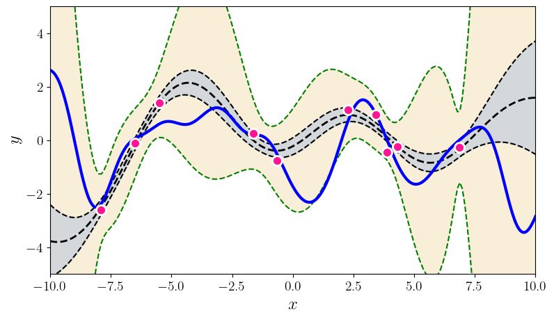
U NCERTAINTY QUANTIFICATION USING MARTINGALES FOR MISSPECIFIED G AUSSIAN PROCESSES

  (C) philosophical, trading a (Bayesian) subjective belief in the prior (γ → ∞) with (frequentist)
       robustness against misspecification (γ → 0).
Returning to our simulation, the confidence sequence guarantees derived at γ = 0 provide robustness
against arbitrary misspecification of the prior, but our choice of γ = 10−2 seemed more reasonable
if we think the prior is not completely ridiculous. An interesting direction for future work is to figure
out how to automatically tune γ in light of the aforementioned tradeoffs.
(3) Compute the confidence sequence. We can then use the confidence sequence
                                                     e−1 (f ) > α}.
                                  Ct = {f ∈ R|Gt | : Rt

    Thus we know that Ct is an ellipsoid defined by the superlevel set of R   e−1 (f ). To compute Ct ,
                                                                                t
we can traverse outwards from the posterior-prior ratio mean µc until we have found the Mahalanobis
distance k to the isocontour I = {f ∈ R|Gt | : cN (f |µc , Σc ) = α}.
    We can therefore view Ct as the k-sigma ellipsoid of the posterior GP (normal distribution) given
by N (f |µc , σc )). Using this confidence ellipsoid over f , we can compute a lower confidence bound
for the value of f (X 0 ), which we use as a LCB-style acquisition function ϕt (x) at input X 0 .
    To summarize the detailed explanations, our simulations use:

                      et (f ) = GP0 (f ) = GP0 (f ) GP0 (f ) = Rt (f ) GP0 (f ) ,
                                f                   f                  f
                      R
                                GPt (f )   GPt (f ) GP0 (f )           GP0 (f )
      f 0 (f ) is the same as GP0 (f ), except with the signal variance parameter σ 2 set to σ 2 (1 + γ).
where GP
BO simulations: GP-LCB versus CS-LCB. We demonstrate BO using Ct (following the pro-
cedure outlined above, which we call CS-LCB) and compare it against the GP-LCB algorithm.
Results for these experiments are given in Appendix A. Briefly, we applied these methods to optimize
an unknown function f ∗ in both the well-specified and misspecified settings. The findings were
as expected: under a misspecified prior, GP-LCB is overconfident about its progress and fails to
minimize f ∗ , while CS-LCB mitigates the issue. For a well-specified prior, both algorithms find the
minimizer, but GP-LCB finds it sooner than CS-LCB.
Robustness to misspecified likelihood. Throughout this paper, we have assumed correctness of
the likelihood model (2), but what if that assumption is suspect? In the supplement, we repeat
the experiment in Figure 1, except when the true noise η ∗ is half the value η used by the working
likelihood (Figure 5), as well as when η ∗ is double of η (Figure 6). As expected, when the noise is
smaller than anticipated, our CS remains robust to the prior misspecification, but when the noise
is larger, we begin to notice failures in our CS. We propose a simple fix: define Řt := Rtβ , for
some β ∈ (0, 1), and construct the CS based on Řt . Figure 7 uses β = 0.75 and reports promising
results. This procedure is inspired by a long line of work in Bayesian inference that proposes raising
likelihoods to a power less than one in order to increase robustness (Ibrahim and Chen, 2000; Royall
and Tsou, 2003; Grünwald, 2012; Grünwald and Van Ommen, 2017; Miller and Dunson, 2019;
Wasserman et al., 2020). Since we desire frequentist coverage guarantees for a Bayesian working
model (not assuming correctness of a Bayesian prior), we simply point out that Řt is not a martingale
like Rt , and is instead a supermartingale due to Jensen’s inequality. Since Ville’s inequality applies,
the resulting CS is still valid. Thus it appears at first glance, that one can obtain some amount of
robustness against both misspecified priors and likelihoods. However, as mentioned below, merging
this idea with hyperparameter tuning and a data-dependent choice of β seems critical for practice.

                                                   10
U NCERTAINTY QUANTIFICATION USING MARTINGALES FOR MISSPECIFIED G AUSSIAN PROCESSES
5. Discussion
Confidence sequences were introduced and studied in depth by Robbins along with Darling, Siegmund
and Lai (Darling and Robbins, 1967; Robbins and Siegmund, 1970; Lai, 1976a,b). The topic
was subsequently somewhat dormant but came back into vogue due to applications to best-arm
identification in multi-armed bandits (Jamieson et al., 2014). Techniques related to nonnegative
supermartingales, the mixture method, Ville’s inequality, and nonparametric confidence sequences
have been studied very recently — see Howard et al. (2020, 2021); Kaufmann and Koolen (2018);
Howard and Ramdas (2019); Waudby-Smith and Ramdas (2020a,b) and references therein. They are
closely tied to optional stopping, continuous monitoring of experiments and scientific reproducibility
(Wald, 1947; Balsubramani, 2014; Balsubramani and Ramdas, 2016; Johari et al., 2017; Shafer et al.,
2011; Grünwald et al., 2019; Howard et al., 2021). We are unaware of other work that utilizes them
to quantify uncertainty in a BO context.
Many important open questions remain. We describe three directions:
• Hyperparameter tuning. It is common in BO practice to tune hyperparameters on the fly
(Snoek et al., 2012; Shahriari et al., 2015; Kandasamy et al., 2020; Neiswanger et al., 2019).
These can alleviate some problems mentioned in the first page of this paper, but probably only if
the kernel is a good match and the function has homogeneous smoothness. We would like to
explore if hyperparameter tuning can be integrated into confidence sequences.
The manner in which we estimate hyperparameters is critical, as highlighted by the recent
work of Bachoc (2018) who asks: what happens when we estimate hyperparameters of our
kernel using (A) maximum likelihood estimation, or (B) cross-validation, when restricting our
attention to some prespecified set of hyperparameters which do not actually capture the true
covariance function? The answer turns out to be subtle: the Maximum Likelihood estimator
asymptotically minimizes a Kullback-Leibler divergence to the misspecified parametric set,
while Cross Validation asymptotically minimizes the integrated square prediction error; Bachoc
demonstrates that the two approaches could be rather different in practice.
• The belief parameter γ. Can γ be tuned automatically, or updated in a data-dependent way?
Further, if we move to the aforementioned hyperparameter tuning setup, can we design a belief
parameter γ that can smoothly trade off our belief in the tuned prior against robustness to
misspecification? Perhaps we would want γ → ∞ with sample size so that as we get more data
to tune our priors better, we would need less robustness protection. Further, perhaps we may
wish to use a convex combination of kernels, with a weight of 1/(1 + γ) for a simpler kernel
(like Gaussian) and a weight of γ/(1 + γ) for a more complex kernel, so that as γ → ∞, we not
only have more faith in our prior, but we may also allow more complex functions.
• Computationally tractable choices for F. While the method introduced in Section 3 is general,
some care had to be taken when instantiating it in the experiments of Section 4, because the
choice of function class F had to be chosen to make computation of the set Ct easy. Can we
expand the set of computational tools so that these ideas are applicable for other choices of F?
How do we scale these methods to work in high dimensions?
The long-term utility of our new ideas will rely on finding suitable answers to the above questions.
There are other recent works that study the mean-squared error of GPs under prior misspecifica-
tion (Beckers et al., 2018), or under potentially adversarial noise in the observation model (Bogunovic
11U NCERTAINTY QUANTIFICATION USING MARTINGALES FOR MISSPECIFIED G AUSSIAN PROCESSES
et al., 2020). Their goals are orthogonal to ours (uncertainty quantification), but a cross-pollination
of ideas may be beneficial to both efforts.
We end with a cautionary quote from Freedman’s Wald lecture (Freedman, 1999):
With a large sample from a smooth, finite-dimensional statistical model, the Bayes
estimate and the maximum likelihood estimate will be close. Furthermore, the posterior
distribution of the parameter vector around the posterior mean must be close to the
distribution of the maximum likelihood estimate around truth: both are asymptotically
normal with mean 0, and both have the same asymptotic covariance matrix. That is the
con- tent of the Bernstein–von Mises theorem. Thus, a Bayesian 95%-confidence set
must have frequentist coverage of about 95%, and conversely. In particular, Bayesians
and frequentists are free to use each other’s confidence sets. However, even for the
simplest infinite-dimensional models, the Bernstein–von Mises theorem does not hold
(see Cox (Cox, 1993))...The sad lesson for inference is this. If frequentist coverage
probabilities are wanted in an infinite-dimensional problem, then frequentist coverage
probabilities must be computed. Bayesians, too, need to proceed with caution in the
infinite-dimensional case, unless they are convinced of the fine details of their priors.
Indeed, the consistency of their estimates and the coverage probability of their confidence
sets depend on the details of their priors.
Our experiments match the expectations set by the above quote: while the practical appeal of
Bayesian credible posterior GP intervals is apparent—they are easy to calculate and visualize—they
appear to be inconsistent under even minor prior misspecification (Figure 1), and this is certainly
seems to be an infinite-dimensional issue. It is perhaps related to the fact that there is no analog
of the Lebesgue measure in infinite dimensions, and thus our finite-dimensional intuition that “any
Gaussian prior puts nonzero mass everywhere” does not seem to be an accurate intuition in infinite
dimensions.
Acknowledgments
AR thanks Akshay Balsubramani for related conversations. AR acknowledges funding from an
Adobe Faculty Research Award, and an NSF DMS 1916320 grant. WN was supported by U.S.
Department of Energy Office of Science under Contract No. DE-AC02-76SF00515.
References
François Bachoc. Asymptotic analysis of covariance parameter estimation for gaussian processes in
the misspecified case. Bernoulli, 24(2):1531–1575, 2018.
Akshay Balsubramani. Sharp finite-time iterated-logarithm martingale concentration. arXiv preprint,
arXiv:1405.2639, 2014.
Akshay Balsubramani and Aaditya Ramdas. Sequential nonparametric testing with the law of the
iterated logarithm. In Proceedings of the Thirty-Second Conference on Uncertainty in Artificial
Intelligence, 2016.
T. Beckers, J. Umlauft, and S. Hirche. Mean square prediction error of misspecified gaussian process
models. In IEEE Conference on Decision and Control (CDC), 2018.
12U NCERTAINTY QUANTIFICATION USING MARTINGALES FOR MISSPECIFIED G AUSSIAN PROCESSES
Julien Bect, François Bachoc, and David Ginsbourger. A supermartingale approach to Gaussian
process based sequential design of experiments. Bernoulli, 25(4A):2883–2919, 2019.
Ilija Bogunovic, Andreas Krause, and Scarlett Jonathan. Corruption-tolerant Gaussian process bandit
optimization. In International Conference on Artificial Intelligence and Statistics (AISTATS),
2020.
Dennis D Cox. An analysis of Bayesian inference for nonparametric regression. The Annals of
Statistics, pages 903–923, 1993.
Donald A. Darling and Herbert Robbins. Confidence sequences for mean, variance, and median.
Proceedings of the National Academy of Sciences, 58(1):66–68, 1967.
David Freedman. Wald Lecture: On the Bernstein-von Mises theorem with infinite-dimensional
parameters. The Annals of Statistics, 27(4):1119–1141, 1999.
Peter Grünwald. The safe Bayesian. In International Conference on Algorithmic Learning Theory,
pages 169–183. Springer, 2012.
Peter Grünwald and Thijs Van Ommen. Inconsistency of Bayesian inference for misspecified linear
models, and a proposal for repairing it. Bayesian Analysis, 12(4):1069–1103, 2017.
Peter Grünwald, Rianne de Heide, and Wouter Koolen. Safe testing. arXiv:1906.07801, June 2019.
Steven R Howard and Aaditya Ramdas. Sequential estimation of quantiles with applications to
A/B-testing and best-arm identification. arXiv preprint arXiv:1906.09712, 2019.
Steven R Howard, Aaditya Ramdas, Jon McAuliffe, and Jasjeet Sekhon. Time-uniform Chernoff
bounds via nonnegative supermartingales. Probability Surveys, 17:257–317, 2020.
Steven R Howard, Aaditya Ramdas, Jon McAuliffe, and Jasjeet Sekhon. Time-uniform, nonparamet-
ric, nonasymptotic confidence sequences. The Annals of Statistics, 2021.
Joseph G Ibrahim and Ming-Hui Chen. Power prior distributions for regression models. Statistical
Science, 15(1):46–60, 2000.
Kevin Jamieson, Matthew Malloy, Robert Nowak, and Sébastien Bubeck. lil’ UCB: An optimal
exploration algorithm for multi-armed bandits. In Proceedings of The 27th Conference on Learning
Theory, volume 35, pages 423–439, 2014.
Ramesh Johari, Pete Koomen, Leonid Pekelis, and David Walsh. Peeking at A/B tests: Why it matters,
and what to do about it. In Proceedings of the 23rd ACM SIGKDD International Conference on
Knowledge Discovery and Data Mining, pages 1517–1525, 2017.
Kirthevasan Kandasamy, Karun Raju Vysyaraju, Willie Neiswanger, Biswajit Paria, Christopher R
Collins, Jeff Schneider, Barnabas Poczos, and Eric P Xing. Tuning hyperparameters without grad
students: Scalable and robust Bayesian optimisation with Dragonfly. Journal of Machine Learning
Research, 21(81):1–27, 2020.
Emilie Kaufmann and Wouter Koolen. Mixture martingales revisited with applications to sequential
tests and confidence intervals. arXiv:1811.11419, 2018.
13U NCERTAINTY QUANTIFICATION USING MARTINGALES FOR MISSPECIFIED G AUSSIAN PROCESSES
Tze Leung Lai. Boundary crossing probabilities for sample sums and confidence sequences. The
Annals of Probability, 4(2):299–312, 1976a.
Tze Leung Lai. On Confidence Sequences. The Annals of Statistics, 4(2):265–280, 1976b.
Jeffrey W Miller and David B Dunson. Robust Bayesian inference via coarsening. Journal of the
American Statistical Association, 114(527):1113–1125, 2019.
Jonas Mockus, Vytautas Tiesis, and Antanas Zilinskas. The application of bayesian methods for
seeking the extremum. Towards global optimization, 2(117-129):2, 1978.
Willie Neiswanger and Eric Xing. Post-inference prior swapping. In Proceedings of the 34th
International Conference on Machine Learning-Volume 70, pages 2594–2602. JMLR. org, 2017.
Willie Neiswanger, Kirthevasan Kandasamy, Barnabas Poczos, Jeff Schneider, and Eric Xing. Probo:
a framework for using probabilistic programming in Bayesian optimization. arXiv preprint
arXiv:1901.11515, 2019.
Herbert Robbins and David Siegmund. Boundary crossing probabilities for the Wiener process and
sample sums. The Annals of Mathematical Statistics, 41(5):1410–1429, 1970.
Richard Royall and Tsung-Shan Tsou. Interpreting statistical evidence by using imperfect models:
robust adjusted likelihood functions. Journal of the Royal Statistical Society: Series B (Statistical
Methodology), 65(2):391–404, 2003.
Eric Schulz, Maarten Speekenbrink, José M Hernández-Lobato, Zoubin Ghahramani, and Samuel J
Gershman. Quantifying mismatch in Bayesian optimization. In NIPS workshop on Bayesian
optimization: Black-box optimization and beyond, 2016.
Glenn Shafer and Vladimir Vovk. Game-Theoretic Foundations for Probability and Finance, volume
455. John Wiley & Sons, 2019.
Glenn Shafer, Alexander Shen, Nikolai Vereshchagin, and Vladimir Vovk. Test martingales, Bayes
factors and p-values. Statistical Science, 26(1):84–101, 2011.
Bobak Shahriari, Kevin Swersky, Ziyu Wang, Ryan P Adams, and Nando De Freitas. Taking the
human out of the loop: A review of Bayesian optimization. Proceedings of the IEEE, 104(1):
148–175, 2015.
Jasper Snoek, Hugo Larochelle, and Ryan P Adams. Practical Bayesian optimization of machine
learning algorithms. In Advances in Neural Information Processing Systems, pages 2951–2959,
2012.
Peter Sollich. Gaussian process regression with mismatched models. In Advances in Neural
Information Processing Systems, pages 519–526, 2002.
Niranjan Srinivas, Andreas Krause, Sham Kakade, and Matthias Seeger. Gaussian process opti-
mization in the bandit setting: no regret and experimental design. In Proceedings of the 27th
International Conference on Machine Learning, pages 1015–1022, 2010.
J Ville. Étude Critique de la Notion de Collectif (PhD Thesis). Gauthier-Villars, Paris, 1939.
14U NCERTAINTY QUANTIFICATION USING MARTINGALES FOR MISSPECIFIED G AUSSIAN PROCESSES
Abraham Wald. Sequential Analysis. John Wiley & Sons, New York, 1947.
Larry Wasserman, Aaditya Ramdas, and Sivaraman Balakrishnan. Universal inference. Proceedings
of the National Academy of Sciences, 2020.
Ian Waudby-Smith and Aaditya Ramdas. Estimating means of bounded random variables by betting.
arXiv preprint arXiv:2010.09686, 2020a.
Ian Waudby-Smith and Aaditya Ramdas. Confidence sequences for sampling without replacement.
Advances in Neural Information Processing Systems, 33, 2020b.
Christopher KI Williams and Carl E Rasmussen. Gaussian processes for machine learning, volume 2.
MIT press Cambridge, MA, 2006.
15U NCERTAINTY QUANTIFICATION USING MARTINGALES FOR MISSPECIFIED G AUSSIAN PROCESSES
Appendix A. Bayesian Optimization Simulations
We demonstrate BO using our confidence sequence Ct (following the procedure outlined in Sec-
tion 4.2) and compare it against the GP-LCB algorithm. Results for these experiments are shown
below, where we apply these methods to optimize a function f in both the misspecified prior (Fig-
ure 2) and correctly specified prior (Figure 3) settings. We find that under a misspecified prior,
GP-LCB can yield inaccurate confidence bands and fail to find the optimum of f , while BO using Ct
(CS-LCB) can help mitigate this issue.
16U NCERTAINTY QUANTIFICATION USING MARTINGALES FOR MISSPECIFIED G AUSSIAN PROCESSES
Figure 2: This figure shows GP-LCB (left column) and CS-LCB (right column) for a misspecified
prior, showing t = 3, 7, 18, 25 (rows 1-4). Here, GP-LCB yields inaccurate confidence bands,
repeatedly queries at the wrong point (around x = 10.0), and fails to find the minimizer of f , while
CS-LCB successfully finds the minimizer (around x = −3.0).
17U NCERTAINTY QUANTIFICATION USING MARTINGALES FOR MISSPECIFIED G AUSSIAN PROCESSES
Figure 3: This figure shows GP-LCB (left column) and CS-LCB (right column) for a correctly
specified prior, showing t = 3, 7, 18, 25 (rows 1-4). Here, both methods find the minimizer of f ,
though GP-LCB has tighter confidence bands and finds the minimizer sooner than CS-LCB.
18U NCERTAINTY QUANTIFICATION USING MARTINGALES FOR MISSPECIFIED G AUSSIAN PROCESSES
Two dimensional benchmark function We also perform a Bayesian optimization experiment
on the two dimensional benchmark Branin function.2 In this experiment, we first run Bayesian
optimization using the GP-LCB algorithm on a model with a misspecified prior, setting {` = 7, σ 2 =
0.1}, and compare it with our CS-LCB algorithm. In both cases, we run each algorithms for 50 steps,
and repeat each algorithm over 10 different seeds. We plot results of both algorithms in Fig. 4, along
with the optimal objective value. We find that in this misspecified prior setting, CS-LCB converges
to the minimal objective value more quickly than GP-LCB.
Branin
2.5
GP-LCB
CS-LCB
Optimal f ∗ (x)
2.0
Minimum queried f (x)
1.5
1.0
0.5
0.0
0 10 20 30 40 50
Iteration
Figure 4: Bayesian optimization using CS-LCB and GP-LCB on the Branin function.
2. Details about this function can be found here: https://www.sfu.ca/~ssurjano/branin.html
19U NCERTAINTY QUANTIFICATION USING MARTINGALES FOR MISSPECIFIED G AUSSIAN PROCESSES
Appendix B. Misspecified Likelihood: low/high noise, and powered likelihoods
We next demonstrate BO in the setting where the likelihood is misspecified. In particular, we are
interested in the setting where the model assumes noise η, which is not equal to the true noise η ∗
from which the data is generated. In this case, we demonstrate the fix proposed in Section 4, using
powered likelihoods. We show results of this adjustment by repeating the experiment of Figure 1 for
η > η ∗ (Figure 5) and η < η ∗ (Figures 6 and 7).
Figure 5: [Low noise setting] We repeat the experiment of Figure 1, but with the true noise η ∗ of
the data being one quarter of the assumed noise η in the working model likelihood (2). Perhaps as
expected, the observed behavior is almost indistinguishable from Figure 1 for both the standard GP
posterior, which remains incorrectly overconfident, and our method, which covers the true function
at all times.
20U NCERTAINTY QUANTIFICATION USING MARTINGALES FOR MISSPECIFIED G AUSSIAN PROCESSES
Figure 6: [High noise setting] We repeat the experiment of Figure 1, but with the true noise η ∗ of the
data being four times the assumed noise η in the working model likelihood (2). In these plots, we
can see incorrect confidence estimates for our prior-robust CS—for example, when the number of
observations t = 10 (second row, first column), and when t = 20 (second row, second column). As
expected, our prior-robust CS is not robust to misspecification of the likelihood.
21U NCERTAINTY QUANTIFICATION USING MARTINGALES FOR MISSPECIFIED G AUSSIAN PROCESSES
Figure 7: [High-noise setting with our ‘powered likelihood’ CS] We consider the same setting of
Figure 6 when the noise of the data is multiplied by four while the assumed noise in the working
model likelihood remains the same. Here, we use a powered likelihood of β = 0.75 for a more robust
confidence sequence, as described at the end of Section 4. Note that the earlier issues at t = 10
(second row, first column) and t = 20 (second row, second column) are now resolved.
22You can also read